∎

Homoclinic dynamics in a spatial restricted four body problem Thanks: The second author was partially supported by NSF grant DMS-1813501. Both authors were partially supported by NSF grant DMS-1700154 and by the Alfred P. Sloan Foundation grant G-2016-7320

blue skies into Smale horseshoes for vertical Lyapunov families

Maxime Murray J.D. Mireles James Affiliation: Florida Atlantic University, Department of Mathematical Sciences E-mail: jmirelesjames@fau.edu

Received: date / Accepted: date

Abstract

The set of transverse homoclinic intersections for a saddle-focus equilibrium in the planar equilateral restricted four body problem admit certain simple homoclinic oribts which form the skeleton of the complete homoclinic intersection – or homoclinic web. In the present work the planar restricted four body problem is viewed as an invariant subsystem of the spatial problem, and the influence of this planar homoclinic skeleton on the spatial dynamics is studied from a numerical point of view. Starting from the vertical Lyapunov families emanating from saddle focus equilibria, we compute the stable/unstable manifolds of these spatial periodic orbits and look for intersections between these manifolds near the fundamental planar homoclinics. In this way we are able to continue all of the basic planar homoclinic motions into the spatial problem as homoclinics for appropriate vertical Lyapunov orbits which, by the Smale Tangle theorem, suggest the existence of chaotic motions in the spatial problem. While the saddle-focus equilibrium solutions in the planar problems occur only at a discrete set of energy levels, the cycle-to-cycle homoclinics in the spatial problem are robust with respect to small changes in energy.

Keywords:

Gravitational

4

- body problem blue sky catastrophes Smale tangle vertical Lyapunov families invariant manifolds boundary value problems

pacs

45.50.Jf 45.50.Pk 45.10.-b 02.60.Lj 05.45.Ac

MSC

70K44 34C45 70F15

1 Introduction

Connecting orbits occupy a central place in the qualitative theory of Hamiltonian systems going back to the groundbreaking work of Poincaré at the dawn of the Twentieth Century MR1194624; MR1194623; MR1194622. Indeed Poincaré’s argument that the circular restricted three body problem (CRTBP) is not integrable relies crucially on the existence of a transverse cycle-to-cycle homoclinic – that is, an orbit which limits in both forward and backward time to a periodic solution. Such an orbit is necessarily in the intersection of the stable and unstable manifolds of the periodic solution, a fact which lends the discussion its distinctively geometric character. The interested reader is referred to the lecture notes of Chenciner MR3329413 for a modern discussion of the theoretical and historical role of invariant manifolds and connecting orbits in Poincaré’s work on the three body problem. In more recent times it has been shown that the existence of transverse homoclinic orbits/heteroclinic cycles implies the existence of chaotic motions quite generally, via the mechanism of Smale MR0228014. The Lectures of Siegel and Moser MR1829194; MR1345153 provide a classic reference on chaotic motions in celestial mechanics.

Inspired by the work of Poincaré, a number of of early Twentieth Century dynamical astronomers – in particular the groups led by Darwin, Strömgren, and Moulton – conducted extensive numerical studies which explored the phase space structure of the CRTBP MR1554890; stromgrenRef; moultonBook. These researchers were especially interested in one parameter families of periodic orbits (“tubes” parameterized by energy) and developed numerical continuation methods to study the global embeddings of these tubes. This work first suggested the importance of saddle-focus libration points, as it was observed that some families of periodic solutions appear to accumulate to an asymptotic cycle – what would be called in modern language a homoclinic orbit – for a saddle-focus libration point. This work provided numerical evidence for the existence of families of periodic orbits in the three body problem which remain bounded in amplitude but nevertheless have period tending to infinity, foreshadowing the canonical work of Chazy in 1922 on the final motions of three body orbits MR1509241.

The advent of digital computing in the mid Twentieth Century facilitated the more detailed numerical studies of Szebehely, Nacozy, and Flandern szebehelyOnStromgren; szebehelyTriangularPoints. A key observation to emerge from this work was that the tubes of periodic orbits mentioned at the end of the previous paragraph appeared to change stability infinitely many times while approaching the homoclinic. This result suggested complicated dynamics near the homoclinic, anticipating the period doubling cascades of Feigenbaum. The interested reader is referred to the work of Pinotsis MR875720; MR742168; MR2726383, as well as the work of Henrard and Navarro MR2104214; MR1956529 and the references therein for more complete discussion.

These developments culminated in 1973 with Henrard’s proof of a theorem which unified the nearly one hundred years of numerical experiments sketched above, finally settling a conjecture of Strömgren about tubes of periodic orbits. More precisely, Henrard showed that the existence of a transverse homoclinic for a saddle-focus equilibrium in a two degrees of freedom Hamiltonian system implies the existence of a tube of periodic orbits parameterized by energy accumulating to the homoclinic MR0365628. Moreover the result established that as the period of the orbits goes to infinity, their stability does indeed change infinitely many times as earlier numerical work suggested. This phenomena – the so called blue sky catastrophe in the terminology of Abraham MR813508 – is studied by a number of authors including L.P. Shilnikov, A.L. Shilnikov, and Turaev MR3253906, and Devaney MR0431274. Indeed Devaney’s 1976 work established that the hypotheses of Henrard’s theorem imply also the existence of chaotic motions in the energy level of the saddle-focus equilibrium MR0442990. We refer to the works of Lerman MR998368; MR1135905 for other theoretical results and discussion, and to the numerical study Gómez, Líbre, and Masdemont in MR993815 which illuminates saddle-focus homoclinic dynamics associated with the $\mathcal{L}_{4,5}$ libration points in the CRTBP.

Theorems like the ones mentioned in the previous paragraph are Hamiltonian versions of the homoclinic bifurcations studied by Shilńikov MR0259275; 0025-5734-10-1-A07; MR0210987, and taken together paint a vivid picture of the rich dynamics near a transverse homoclinic connection for a saddle-focus equilibrium in a two degree of freedom Hamiltonian system. A natural follow up question is what, if anything, do the results about two freedom systems just described tell us about Hamiltonian systems with three or more degrees of freedom? The question is reasonable as many problems in celestial mechanics have an invariant planar subsystem due to the conservation of angular momentum.

The present work considers this question in the context of a spatial equilateral restricted four body problem, hereafter referred to as the circular restricted four body problem (CRFBP). The equations of motion, as well as some history and basic properties of the problem are reviewed in Section 2. The problem is an excellent candidate for the present study as the homoclinic dynamics in the invariant planar subsystem have recently been studied in some detail. In particular, the work of Shane Kepley and the second author MR3919451 provides a detailed numerical study of blue sky catastrophes in the case of equal masses. The main observation is that the saddle-focus homoclinics appear to be organized by a small number of simple connections, or homoclinic channels. In fact these channels are just the “shortest” homoclinics (see MR3919451 for the precise meaning of shortest in this context), and there turn out to be six of them at each saddle-focus equilibrium in the CRFBP. If one considers these six shortest homoclinic connections as the letters of a symbolic alphabet, then all the other homoclinic connections – of which there appear to be infinitely many – organize themselves into “words” in this alphabet. In short the homoclinic web at any saddle focus in the CRFBP appears to be organized by six fondamental motions. The results of MR3919451 are reviewed in Section 2.2.

When the planar CRFBP is viewed as a subsystem of the spatial CRFBP the spectrum of a libration point picks up an additional center direction, and there is an out of plane family of periodic orbits associated with each of the planar libration points. These are the so called vertical Lyapunov families and they inherit the stability of the planar librations. We are particularly interested in the vertical families associated with the saddle-focus equilibrium solutions, where the stable/unstable manifolds of the vertical periodic orbits are three dimensional with complex conjugate stable/unstable Floquet multipliers.

The system conserves the so called Jacobi integral, so that any fixed vertical Lyapunov orbit and its attached three dimensional stable/unstable manifolds live in a five dimensional level set, and the dimension count allows for the possibility of transverse intersections between the stable/unstable manifolds relative to the integral manifold. If such an intersection actually occurs, it follows from the Smale tangle theorem MR0228014 that there is a chaotic subsystem near the connecting orbit.

The present work provides compelling numerical evidence in support of the claim that the planar homoclinic orbits studied in MR3919451 give rise to transverse homoclinic orbits, and hence Smale tangles, for the corresponding vertical Lyapunov families in the spatial CRFBP. That is, we find a six letter homoclinic alphabet for the spatial cycle-to-cycle connections, inherited from the planar problem. The out of plane connections appear to persist for fairly large out of plane amplitudes.

In all of our computations we utilize the parameterization method to approximate the stable/unstable manifolds of the Lyapunov orbits in large region surrounding the periodic orbit. The parameterization method is reviewed in Section 3, in particular a number of references to the literature are given there. Connecting orbits are then located as solutions of two point boundary value problems with boundary conditions projected onto the parameterization of the local stable/unstable manifolds. The virtue of using the parameterization method in the present context is that it stabilizes the numerics, leading to a better condition number in the two point boundary value problem. This is especially valuable when, as in the present work, we are trying to find many connections as the same local parameterizations can be used to formulate the BVPs for all the connecting orbits.

The remainder of the paper is organized as follows. In Section 2 we review the CRFBP and discuss some basic results from the literature. In particular we review the findings of MR3919451 on homoclinic channels in the planar problem and also introduce the vertical Lyapunov families which are the main objects of the present study. In Section 3 we review the parameterization method and derive the homological equations which determine the Fourier-Taylor coefficients of the local invariant manifold approximations and discuss our implementations. Section 4 describes briefly the formulation of the two point boundary value problems for cycle-to-cycle connections, and in Section 5 we present the main results of the paper – numerical calculations of the homoclinic connections for the the vertical Lyapunov family in the CRFBP. In Section 6 we summarize our conclusions. We provide two appendices. One is Section A describing the “automatic differentiation” framework which reduces the problem to polynomial, and the other is Section B which tabulates for the sake of reproducibility some of the data produced in the present study.

2 The restricted four body problem

In this section, we introduce the particular version of the four body problem studied in the present work. We postpone to Section 2.1 discussion of the equations of motion, and give first a brief overview of the literature surrounding the problem, which originates from the work of Pedersen pedersen1; pedersen2. Detailed numerical studies of the equilibrium set as well as the planar and spatial Hill’s regions are found in the works of Simó MR510556, Baltagiannis and Papadakis MR2845212, and Álvarez-Ramíerz and Vidal MR2596303. Mathematically rigorous theorems about the equilibrium set and its bifurcations are proven with computer assistance by Leandro and Barros in MR2232439; MR2784870; MR3176322. The papers just cited establish that for any value of the primary masses there are always either 8, 9, or 10 equilibrium solutions (or libration points) with 6 outside the equilateral triangle formed by the primary bodies (see Figure 1).

Periodic orbits are studied by Papadakis in MR3571218; MR3500916, and by Burgos-García, Bengochea, and Delgado in burgosTwoEqualMasses; MR3715396. A computer assisted study by Burgos-García, Lessard, and Mireles James proves the existence of some spatial periodic orbits for the CRFBP jpJaimeAndMe. Regularization of collisions are studied by Álvarez-Ramírez, Delgado, and Vidal in MR3239345. Chaotic motions were studied numerically by Gidea and Burgos in MR2013214, and by Álvarez-Ramírez and Barrabés in MR3304062.

Perturbative proofs of the existence of chaotic motions are found in the work of She, Cheng and Li MR3626383; MR3158025; MR3038224, and also in the work of Alvarez-Ramírez, García, Palacián, and Yanguas chaosCRFBP. A Hill’s problem is derived from the CRFBP and its periodic orbits are studied by Burgos-García and Gidea in MR3554377; MR3346723.

Blue sky catastrophes in the CRFBP are studied by Burgos-García and Delgado in MR3105958, and by Kepley and Mireles James in shaneAndJay. This last reference develops computer assisted methods of proof for verifying the hypotheses of the theorems of Hernard and Devaney. The authors of the last reference cited further study the blue sky catastrophes for the CRFBP in MR3919451, as discussed already in the introduction.

Refer to caption — Figure 1: Configuration space for the CRFBP: The three primary bodies with masses $m_{1},m_{2},$ and $m_{3}$ are arranged in the equilateral triangle configuration of Lagrange – a relative equilibrium solution of the three body problem. Transforming to a co-rotating frame one considers the motion of a fourth massless body. The equations of motion have $8$ , $9$ , or $10$ equilibrium solutions denoted by $\mathcal{L}_{j}$ for $0\leq j\leq 9$ . The number of libration points, and their stability, varies depending on $m_{1}$ , $m_{2}$ , and $m_{3}$ . In this work we study the points $\mathcal{L}_{0,4,5,6}$ which have saddle focus stability when $m_{1}\approx m_{2}\approx m_{3}$ .

2.1 Equations of motion and libration points for the CRFBP

The problem describes the motion of a massless particle moving under the influence of three massive bodies called the primaries. The primaries have masses $m_{1}$ , $m_{2}$ and $m_{3}$ , and are constrained to move in the equilateral triangle configuration of Lagrange. The masses of the primaries are normalized so that $0<m_{3}\leq m_{2}\leq m_{1}$ , and

m_{1}+m_{2}+m_{3}=1,

and the problem is studied in co-rotating coordinate system. The coordinates are chosen so that the center of mass of the primaries is at the origin, the largest primary is fixed on the $x$ -axis, the $x$ -axis cuts the side of the triangle opposite the largest primary and the smallest primary is in the first quadrant.

Under these constraints the location of the primaries is a function of only the choice of masses. To see this let $p_{i}$ denote the position of the $i-$ th primary and write

p_{1}=(x_{1},y_{1},z_{1}),\quad\quad p_{2}=(x_{2},y_{2},z_{2}),\quad\quad\text{and}\quad\quad p_{3}=(x_{3},y_{3},z_{3}),

then

	$\displaystyle x_{1}$	$\displaystyle=$	$\displaystyle\frac{-\|K\|\sqrt{m_{2}^{2}+m_{2}m_{3}+m_{3}^{2}}}{K}$
	$\displaystyle y_{1}$	$\displaystyle=$	$\displaystyle 0$

	$\displaystyle x_{2}$	$\displaystyle=$	$\displaystyle\frac{\|K\|\left[(m_{2}-m_{3})m_{3}+m_{1}(2m_{2}+m_{3})\right]}{2K\sqrt{m_{2}^{2}+m_{2}m_{3}+m_{3}^{2}}}$
	$\displaystyle y_{2}$	$\displaystyle=$	$\displaystyle\frac{-\sqrt{3}m_{3}}{2m_{2}^{3/2}}\sqrt{\frac{m_{2}^{3}}{m_{2}^{2}+m_{2}m_{3}+m_{3}^{2}}},$

	$\displaystyle x_{3}$	$\displaystyle=$	$\displaystyle\frac{\|K\|}{2\sqrt{m_{2}^{2}+m_{2}m_{3}+m_{3}^{2}}}$
	$\displaystyle y_{3}$	$\displaystyle=$	$\displaystyle\frac{\sqrt{3}}{2\sqrt{m_{2}}}\sqrt{\frac{m_{2}^{3}}{m_{2}^{2}+m_{2}m_{3}+m_{3}^{2}}},$

and

z_{1}=z_{2}=z_{3}=0,

where

K=m_{2}(m_{3}-m_{2})+m_{1}(m_{2}+2m_{3}).

Define the potential function

\Omega(x,y,z):=\frac{1}{2}(x^{2}+y^{2})+\frac{m_{1}}{r_{1}(x,y,z)}+\frac{m_{2}}{r_{2}(x,y,z)}+\frac{m_{3}}{r_{3}(x,y,z)},

where $r_{i}$ represents the distance between the massless body and the $i-$ th primary, so that

r_{1}(x,y,z):=\sqrt{(x-x_{1})^{2}+(y-y_{1})^{2}+(z-z_{1})^{2}},

r_{2}(x,y,z):=\sqrt{(x-x_{2})^{2}+(y-y_{2})^{2}+(z-z_{2})^{2}},

and

r_{3}(x,y,z):=\sqrt{(x-x_{3})^{2}+(y-y_{3})^{2}+(z-z_{3})^{2}}.

The equations of motion in the co-rotating coordinates are

\begin{split}\ddot{x}-2\dot{y}&=\Omega_{x},\\ \ddot{y}+2\dot{x}&=\Omega_{y},\\ \ddot{z}&=\Omega_{z}.\end{split}

(1)

The system admits between $8$ and $10$ equilibrium solutions depending on the value of mass ratio, all of them lying in the $xy-$ plane. Closed form formulas for the locations of the equilibrium solutions do not exist and in practice it is necessary to numerically compute their locations once the mass ratios are fixed. A schematic describing the locations of the 10 equilibrium points along with our naming conventions in the case when the $m_{1}\approx m_{2}\approx m_{3}$ , is given in Figure 1.

2.2 Homoclinic dynamics in the planar problem

In this section we describe the homoclinic dynamics associated with the saddle-focus equilibrium solutions in the case that $m_{1}=m_{2}=m_{3}=1/3$ . We refer to this as the triple Copenhagen problem, as the case of equal masses in the CRTBP is traditionally referred to as the Copenhagen problem. The material in this section is discussed in much more detail in MR3919451, on which the present work builds.

The local invariant manifold structure in the triple Copenhagen problem is illustrated in Figure 2. The Figure depicts the fact that $\mathcal{L}_{j}$ for $j=1,2,3,7,8,9$ have saddle $\times$ center type stability. Because of this, there is a planar family of Lyapunov orbits associated with these libration points. The periodic orbits foliate the attached center manifolds, and are illustrated by concentric blue circles in the Figure 2.

When $j=0,4,5,6$ the libration points have saddle-focus stability. That is, each of these libration points have a complex conjugate pair of stable and a complex conjugate pair of unstable eigenvalues. The attached two dimensional stable and unstable manifolds are foliated by orbits which converge exponentially to the libration point in forward and backward time. The 2D stable/unstable orbits are illustrated by the green (unstable) and red (stable) curves respectively, and give a sense of the location of the local stable/unstable manifolds.

The main topic of MR3919451 is to describe the geometry of the homoclinic web – the set of all intersections between the stable and unstable manifolds – attached to the saddle focus equilibrium solutions in the triple Copenhagen problem. The authors developed and deployed the following search procedure.

•

Step 1: Compute high order polynomial approximations of the local stable/unstable manifolds. Mesh the boundary of the local approximation into a system of one dimensional arcs.
•

Step 2: Extend the local approximations by Taylor integration of the one dimensional boundary arcs for time $\pm\tau$ . Each step of Taylor integration results in a two dimensional manifold patch. After integrating the complete system of arcs the result is a larger local manifold approximation.
•

Step 3: Check the stable against the unstable manifold patches produced in step $2$ for approximate intersections. If none are found then no intersections exist up to time $2\tau$ . If an approximate intersection is found it is verified/refined using a boundary value solver.
•

Repeat: collapse the manifold patches from Step $3$ onto their outer boundaries, obtaining a new system of boundary arcs for the local invariant manifold. Then repeat Steps 2 and 3 as desired. At the end of the $N$ -th step the original local approximations have been extended by time $N\tau$ thus locating all intersections up to time $2N\tau$ .

In practice the scheme described above is combined with sophisticated step size selection and remeshing schemes which insure accuracy and efficiency.

As the algorithm runs all connections it locates are sorted and stored according to the “time of flight” of the orbit – that is, the time it takes for the orbit to transition from the boundary of the initial unstable manifold approximation to the boundary of the initial stable manifold approximation. Comparing times of flight provides a precise notion of “shortest” connections. Complexity of the homoclinic connections can be quantified by computing winding numbers with respect to the primary bodies and the libration points.

Step 1 utilizes the parameterization method as described in MR1976079; MR2177465. See also the book of mamotreto. The stable/unstable manifolds illustrated in Figure 2 were computed using this method.

Step 2 uses the methods of analytic continuation for growing atlases of local stable/unstable invariant manifolds developed in manifoldPaper1. To see an illustration of how the local invariant manifolds grow see in the triple Copenhagen problem at $\mathcal{L}_{0}$ and $\mathcal{L}_{5}$ , see Figures 7 and 8 of MR3919451. Figure 3 illustrates the results of running the algorithm for $\tau=4$ time units, hence locating all homoclinics with time of flight up to $8$ time units (a certain velocity constraint which removes a small neighborhood of each of the primaries is also imposed).

The search procedure resulted in dozens of distinct homoclinic orbits at the libration points $\mathcal{L}_{0}$ and $\mathcal{L}_{5}$ . In the case of equal masses it is sufficient to study only these equilibrium solutions as a rotation by $\pm 120$ degrees transforms $\mathcal{L}_{5}$ into $\mathcal{L}_{4,6}$ respectively. Similarly, at $\mathcal{L}_{0}$ rotation of any homoclinic by $\pm 120$ degrees yields another homoclinic connections.

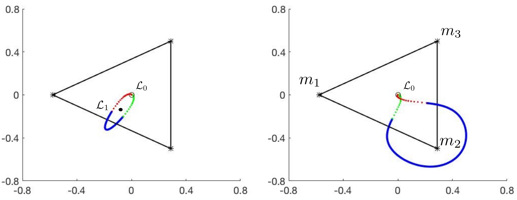
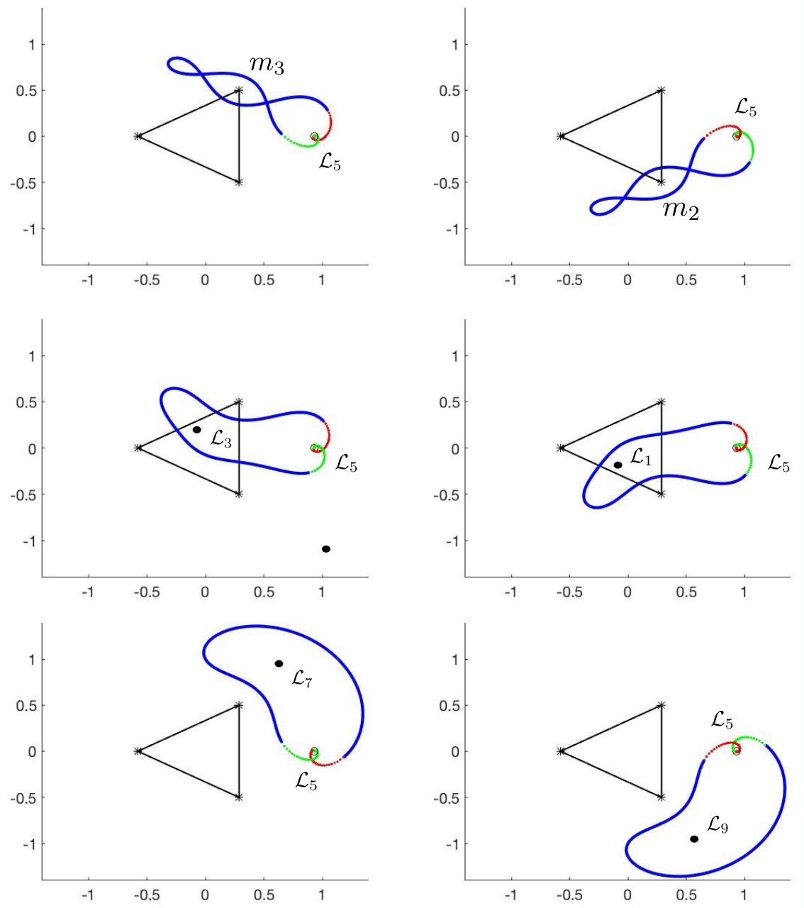
Further examination of the connecting orbits located using the search procedure just described reveals the main result of MR3919451, which is that the homoclinic web at each of the libration points appears to be organized by the six shortest connections. More precisely, each of the six shortest homoclinic orbits can be thought of as a letter in a symbol alphabet, and all of the homoclinic orbits located in the search shadow some combination of these fundamental letters. They are “words” built from the basic alphabet. Put another way, only six fundamental homoclinic motions govern the complete web of connections. The six fundamental homoclinic motions are $\mathcal{L}_{0}$ and $\mathcal{L}_{5}$ are illustrated in Figures 4 and 5 respectively.

2.3 Vertical Lyapunov Families

As mentioned briefly above, the spatial CRFBP inherits the libration points of the planar problem. Moreover, the spatial problem has no out of plane equilibrium solutions. In terms of stability, each planar equilibrium solutions picks up a center direction when embedded in the spatial problem. That is, each of the spatial libration points has a purely imaginary pair of eigenvalues $\pm i\omega$ associated with an out of plane eigenspace. The Lyapunov center theorem MR0021186; MR2189486; MR96021 is used to prove that there is a one parameter family of periodic orbits tangent to the vertical eigenspace of each libration point. The family can be computed by numerical continuation begun in a small neighborhood of the libration point.

The vertical family at $\mathcal{L}_{5}$ for the triple Copenhagen problem is illustrated in Figure 6. Initially the orbits have a “figure eight” shape, with the eight pinched at the libration point and one lobe above and one below the $z=0$ plane. The family is parameterized by energy and as energy is increased the eight opens up and eventually “tips”, returning to the plane. The union of the $\mathcal{L}_{5}$ family forms a sphere in configuration space enclosing the three primaries. The vertical families at $\mathcal{L}_{4,6}$ are obtained by $\pm 120$ degree rotations.

The situation at $\mathcal{L}_{0}$ in the triple Copenhagen problem is illustrated in Figure 7. Due to the symmetry of the problem the $\mathcal{L}_{0}$ vertical family moves entirely on the $z$ -axis. The $\mathcal{L}_{2}$ vertical family is illustrated in the same picture. This family also appears to form a sphere, but in this case the orbits eventually accumulate on the $\mathcal{L}_{0}$ family on the $z$ -axis. The vertical families at $\mathcal{L}_{1,3}$ are obtained by $\pm 120$ degree rotation of the $\mathcal{L}_{2}$ family, and hence all three families accumulate at $\mathcal{L}_{0}$ .

The existence of the spatial periodic orbits illustrated in Figures 6 and 7, along with many other such results, are proven with computer assistance in MR3896998. For small enough out of plane amplitude orbits in the vertical families inherit their stability from the stability of the planar libration point. Then at $\mathcal{L}_{0,4,5,6}$ the vertical Lyapunov orbits have complex conjugate stable/unstable Floquet exponents for some range of out of plane amplitudes.

3 Parameterization of stable/unstable manifolds

In this section we review the parameterization method for stable/unstable manifolds attached to periodic solutions of ordinary differential equations, with an eye toward numerical calculations. Much of the material has appeared in other places, and is included here for the benefit of the reader not familiar with these developments. Indeed it is our hope that the present section provides a useful introduction to the ideas in context if a highly non-trivial application problem. We also stress that a concrete description of the method accompanied by a complete description of the numerical implementation for a periodic orbit in a gravitational $N$ -body problem having complex conjugate Floquet exponents – and hence a three dimensional stable/unstable manifold– has not appeared before. Hence our little tutorial has some novelty. However the reader familiar with this material may want to skip this section upon first reading.

The parameterization method is a functional analytic framework for studying invariant manifolds which is useful in both theoretical and numerical settings. The method has been successfully applied to the study of stable/unstable manifolds attached to fixed points of nonlinear maps between Banach spaces MR1976079; MR1976080, invariant circles and their whiskers in quasi-periodically forced maps, stable/unstable manifolds of normally hyperbolic invariant tori MR2240743; MR2289544; MR2299977, stable/unstable manifolds attached to equilibrium and periodic solutions of parabolic PDEs jpRafPDE; parmPDE, and quasi-periodic solutions and invariant tori in infinite dimensional systems MR2505176; MR2528494; rafaelStDelay_I; rafaelStDelay_II. The parameterization method has also been used to formulate KAM theorems without the use of action angle variables MR2122688; MR2966749, and dissipative KAM theorems MR3062760; MR3095277. Several works focusing on numerical aspects of the method are maximeJPMe; parmChristian; kotParm; fastSlow; MR3068557; MR3032844; MR2507323; jayChrisParmDDE; MR2851901.

We make special mention of the works of MR2177465; MR2551254; MR3118249; doi:10.1137/140960207; poManProofs; chebManifolds. These papers deal with various aspects of the parameterization method for stable/unstable manifolds attached to periodic solutions of differential equations, and are the basis of the approach to invariant manifolds employed in the present work. The rest of the section is devoted to the review of this material.

3.1 Invariance and homological equations

Since the invariant manifolds we consider in the present work have complex Floquet exponents we describe the method in the context of complex vector fields. So, consider the analytic vector field $f:\mathbb{C}^{m}\to\mathbb{C}^{m}$ and the associated first order system of ordinary differential equations $\dot{x}=f(x)$ . Suppose that $\gamma:\mathbb{R}\to\mathbb{C}^{m}$ and $T>0$ have

\frac{d}{dt}\gamma(t)=f(\gamma(t)),

and

\gamma(t+T)=\gamma(t),

for all $t\in\mathbb{R}$ . We say that $\gamma$ is a $T$ -periodic solution of the differential equation.

Assume now that $\gamma$ has $n$ stable (or unstable) Floquet exponents, which we denote by $\lambda_{1},\lambda_{2},\ldots,\lambda_{n}\in\mathbb{C}$ . Let $\mathbb{D}^{n}\subset\mathbb{C}^{n}$ denote the $n$ -dimensional unit poly-disk. Then it is natural to look for a parameterization $P\colon\mathbb{R}\times\mathbb{D}^{n}\to\mathbb{C}^{m}$ – $T$ periodic in the first variable – of the associated stable (or unstable) manifold.

Let $\Lambda$ denote the $n\times n$ diagonal matrix of stable exponents. Then an appropriate model of the stable manifold is the cylinder $\mathbb{S}^{1}\times\mathbb{D}^{n}$ endowed with the linear vector field

K(\theta,\sigma)=\left(\begin{array}[]{c}1\\ \Lambda\sigma\end{array}\right).

Observe that this field has a $1$ -periodic solution at $\sigma=0$ , and that all orbits with $\sigma\neq 0$ converge exponentially to this periodic orbit, making this the simplest possible model for the dynamics on the stable manifold.

The geometric idea behind the parameterization method is to look for a parameterization $P$ satisfying the infinitesimal conjugacy

DP(\theta,\sigma)K(\theta,\sigma)=f(P(\theta,\sigma)).

The equation demands that the push forward of the vector field $K$ by $P$ is equal to the vector field $f$ restricted to the image of $P$ . If the vector fields are equal then they generate the same dynamics (same orbits). But the orbits of $K$ are known explicitly, and we have that any such $P$ parameterizes a local stable manifold for $\gamma$ . The situation is illustrated schematically in Figure 8. Expanding the first order differential operator $DP\circ K$ on the left leads to the invariance equation

\frac{d}{d\theta}P(\theta,\sigma)+\sum_{i=1}^{n}\lambda_{i}\sigma_{i}\frac{\partial}{\partial\sigma_{i}}P(\theta,\sigma)=f(P(\theta,\sigma)),

(2)

which is a first order system of PDEs for $P$ . We impose the first order constraints

P(\theta,0)=\gamma(\theta)

(3)

and

\frac{\partial}{\partial\sigma_{i}}P(\theta,0)=v_{i}(\theta)

for $i=1,2,\ldots,n$ where $v_{i}(\theta)$ – the stable (or unstable) normal bundle associated with the Floquet exponent $\lambda_{i}$ – solves the linear differential equation

-v_{j}(t)^{\prime}+Df(\gamma(t))v_{j}(t)=\lambda_{j}v_{j}(t),

(4)

for each $1\leq j\leq n$ . The function $v_{j}$ is either $T$ periodic or $2T$ periodic depending on wether the associated bundle is orientable or not.

Let $\Phi\colon\mathbb{C}^{m}\times\mathbb{R}\to\mathbb{C}^{m}$ be the flow generated by $f$ . It can be shown (see any of the references given at the end of the last section) that if $P$ is a solution of the infinitesimal invariance Equation (2), then $P$ satisfies the flow conjugacy

\Phi(P(\theta,\sigma),t)=P\left(\theta+t,e^{\Lambda t}\sigma\right),

(5)

for all $t\geq 0$ and $\sigma\in\mathbb{D}^{n}$ . Then in fact the parameterization method recovers the dynamics on the manifold in addition to the embedding.

Since $f$ is analytic we look for an analytic $P$ . To this end suppose that $P$ has the power series expansion

P(\theta,\sigma)=\sum_{|\alpha|=0}^{\infty}A_{\alpha}(\theta)\sigma^{\alpha},

(6)

where for each multi-index $\alpha=(\alpha_{1},\alpha_{2},\ldots,\alpha_{n})\in\mathbb{N}^{\alpha}$ ,

|\alpha|=\alpha_{1}+\alpha_{2}+\ldots+\alpha_{n}

and given $\sigma\in\mathbb{D}^{n}$ we denote

\sigma^{\alpha}=\sigma_{1}^{\alpha_{1}}\cdot\sigma_{2}^{\alpha_{2}}\cdot\ldots\cdot\sigma_{n}^{\alpha_{n}}.

Moreover, each of the coefficients $A_{\alpha}\colon\mathbb{R}\to\mathbb{C}^{m}$ are $\mathbb{T}-$ periodic complex functions. Plugging the expansion (6) in (2) and matching power of $\sigma$ leads to the homological equation for $A_{\alpha}(t)$ given by

\frac{d}{d\theta}A_{\alpha}(\theta)+\langle\alpha,\Lambda\rangle A_{\alpha}(\theta)=f(P(\theta,\sigma))_{\alpha}.

(7)

where

\langle\alpha,\Lambda\rangle=\alpha_{1}\lambda_{1}+\ldots+\alpha_{n}\lambda_{n}.

Remark 1 (Non resonance criteria)

We say that the Floquet exponents $\lambda_{1},\ldots,\lambda_{n}$ are resonant at order $k$ if there exist $\alpha\in\mathbb{N}^{n}$ so that $|\alpha|=k$ and

\langle\alpha,\Lambda\rangle=\lambda_{i}

for some $\lambda_{i}$ a Floquet exponent of $\gamma$ . We recall (see again any of the references cited in the last paragraph of the previous section) that the homological equations are uniquely solvable to all orders if and only if there are no resonances for $|\alpha|\geq 2$ . In this case we say that the Floquet exponents are non-resonant. For the examples considered in the remainder of the paper the periodic orbits had a single complex conjugate pair of stable/unstable Floquet exponents and all the other exponents are purely imaginary. In such a case there is no possibility of resonances for $|\alpha|\geq 2$ , and the parameterization coefficients $A_{\alpha}(\theta)$ are guaranteed to be defined to all orders.

Since solutions of the homological equations are $T$ periodic for all $\alpha$ , it is natural to expand it using Fourier series. Letting $\omega=\frac{2\pi}{T}$ where $T$ is the period of $\gamma$ we look for $A_{\alpha}$ expressed as

A_{\alpha}(\theta)=\sum_{k\in\mathbb{Z}}a_{\alpha,k}e^{\mathrm{i}\omega k\theta}.

Then, one can plug the expansion in (7) and rewrite the problem as the zero of a nonlinear operator defined on the space of Fourier coefficients. The focus of next section is to solve (7) up to some finite order using a finite dimensional Fourier expansion. The process will be explicitly presented in the case of the CRFBP.

3.2 Parameterized manifolds in the CRFBP

Our goal is to solve Equation (7) for the CRFBP. In fact, we use the the idea discussed in Appendix A and first pass to an equivalent polynomial vector field $f\colon\mathbb{R}^{9}\to\mathbb{R}^{9}$ . Having polynomial nonlinearities greatly simplifies the formal series calculations, as Fourier-Taylor series are multiplied as follows.

Suppose that $g,h:[0,T]\times\mathbb{D}^{n}\to\mathbb{C}$ are given by

g(t,\sigma)=\sum_{|\alpha|=0}^{\infty}\sum_{k\in\mathbb{Z}}a_{\alpha,k}e^{\mathrm{i}k\omega t}\sigma^{\alpha},

and

h(t,\sigma)=\sum_{|\alpha|=0}^{\infty}\sum_{k\in\mathbb{Z}}b_{\alpha,k}e^{\mathrm{i}k\omega t}\sigma^{\alpha}.

We refer to $g$ and $h$ as Fourier-Taylor series and to

a=\{a_{\alpha,k}\in\mathbb{C}:\alpha\in\mathbb{N}^{n}~\mbox{and}~k\in\mathbb{Z}\},

and

b=\{b_{\alpha,k}\in\mathbb{C}:\alpha\in\mathbb{N}^{n}~\mbox{and}~k\in\mathbb{Z}\},

as the Fourier-Taylor coefficients of $g$ and $h$ respectively. Observe that $g,h$ are $T$ periodic in $t$ .

Definition 1 (Convolution product)

The Fourier-Taylor series of the point-wise product $g\cdot h(t,\sigma)$ is

(g\cdot h)(t,\sigma)=\sum_{|\alpha|=0}^{\infty}\sum_{k\in\mathbb{Z}}(a\ast b)_{\alpha,k}e^{\mathrm{i}k\omega t}\sigma^{\alpha},

where the Fourier-Taylor coefficients are given by the Cauchy-convolution products

(a\ast b)_{\alpha,k}=\sum_{\begin{subarray}{c}\alpha_{1}+\alpha_{2}=\alpha\\ \alpha_{1},\alpha_{2}\in\mathbb{N}^{n}\end{subarray}}\sum_{\begin{subarray}{c}k_{1}+k_{2}=k\\ k_{1},k_{2}\in\mathbb{Z}\end{subarray}}a_{\alpha_{1},k_{1}}\cdot b_{\alpha_{2},k_{2}}.

We refer to $\ast$ as the Cauchy-convolution product of $a$ and $b$ .

The definition extends also to higher order powers. For example

g^{3}(t,\sigma)=\sum_{|\alpha|=0}^{\infty}\sum_{k\in\mathbb{Z}}(a*a*a)_{\alpha,k}e^{ik\omega t}\sigma^{\alpha},

where

(a*a*a)_{\alpha,k}=\sum_{\begin{subarray}{c}\alpha_{1}+\alpha_{2}+\alpha_{3}=\alpha\\ \alpha_{1},\alpha_{2},\alpha_{3}\in\mathbb{N}^{n}\end{subarray}}\sum_{\begin{subarray}{c}k_{1}+k_{2}+k_{3}=k\\ k_{1},k_{2},k_{3}\in\mathbb{Z}\end{subarray}}a_{\alpha_{1},k_{1}}\cdot a_{\alpha_{2},k_{2}}\cdot a_{\alpha_{3},k_{3}}.

Quartic and quintic powers are defined in the analogous way.

We now look for the Fourier-Taylor coefficients of the stable (or unstable) manifold parameterization, which we write as

P(\theta,\sigma)=\sum_{|\alpha|=0}^{\infty}\sum_{k\in\mathbb{Z}}a_{\alpha,k}e^{i\omega k\theta}\sigma^{\alpha},

where

a_{\alpha,k}=\left(\begin{array}[]{c}a^{1}_{\alpha,k}\\ a^{2}_{\alpha,k}\\ a^{3}_{\alpha,k}\\ a^{4}_{\alpha,k}\\ a^{5}_{\alpha,k}\\ a^{6}_{\alpha,k}\\ a^{7}_{\alpha,k}\\ a^{8}_{\alpha,k}\\ a^{9}_{\alpha,k}\end{array}\right)\in\mathbb{C}^{9},

for each $\alpha\in\mathbb{N}^{n}$ and $k\in\mathbb{Z}$ . Observe that $\{a_{0,k}\}_{k\in\mathbb{Z}}$ and $\{a_{e_{j},k}\}_{k\in\mathbb{Z}}$ are the Fourier coefficients of the periodic orbit and the $j$ -th normal bundle respectively.

After rewriting the CRFBP as a polynomial system (see again Appendix A) and projecting Equation (7) for the resulting polynomial field into Fourier-Taylor coefficient space, we obtain for each $|\alpha|\geq 2$ an equivalent $F_{\alpha}(a)=0$ problem, where $F_{\alpha}$ is the map given by

	$\displaystyle F_{\alpha,k}^{1}(a)=$	$\displaystyle(\mathrm{i}\omega k+\langle\alpha,\lambda\rangle)a_{\alpha,k}^{1}-a_{\alpha,k}^{2},$
	$\displaystyle F_{\alpha,k}^{2}(a)=$	$\displaystyle(\mathrm{i}\omega k+\langle\alpha,\lambda\rangle)a_{\alpha,k}^{2}-2a_{\alpha,k}^{4}-a_{\alpha,k}^{1}+\sum_{i=1}^{3}m_{i}\left((a^{1}-x_{i})\ast a^{6+i}\ast a^{6+i}\ast a^{6+i}\right)_{\alpha,k},$
	$\displaystyle F_{\alpha,k}^{3}(a)=$	$\displaystyle(\mathrm{i}\omega k+\langle\alpha,\lambda\rangle)a_{\alpha,k}^{3}-a_{\alpha,k}^{4},$
	$\displaystyle F_{\alpha,k}^{4}(a)=$	$\displaystyle(\mathrm{i}\omega k+\langle\alpha,\lambda\rangle)a_{\alpha,k}^{4}+2a_{\alpha,k}^{2}-a_{\alpha,k}^{3}+\sum_{i=1}^{3}m_{i}\left((a^{3}-y_{i})\ast a^{6+i}\ast a^{6+i}\ast a^{6+i}\right)_{\alpha,k},$
	$\displaystyle F_{\alpha,k}^{5}(a)=$	$\displaystyle(\mathrm{i}\omega k+\langle\alpha,\lambda\rangle)a_{\alpha,k}^{5}-a_{\alpha,k}^{6},$
	$\displaystyle F_{\alpha,k}^{6}(a)=$	$\displaystyle(\mathrm{i}\omega k+\langle\alpha,\lambda\rangle)a_{\alpha,k}^{6}+\sum_{i=1}^{3}m_{i}\left((a^{5}-z_{i})\ast a^{6+i}\ast a^{6+i}\ast a^{6+i}\right)_{\alpha,k},$
	$\displaystyle F_{\alpha,k}^{7}(a)=$	$\displaystyle(\mathrm{i}\omega k+\langle\alpha,\lambda\rangle)a_{\alpha,k}^{7}+\left(\left((a^{1}-x_{1})\ast a^{2}+(a^{3}-y_{1})\ast a^{4}+(a^{5}-z_{1})\ast a^{6}\right)\ast a^{7}\ast a^{7}\ast a^{7}\right)_{\alpha,k},$
	$\displaystyle F_{\alpha,k}^{8}(a)=$	$\displaystyle(\mathrm{i}\omega k+\langle\alpha,\lambda\rangle)a_{\alpha,k}^{8}+\left(\left((a^{1}-x_{2})\ast a^{2}+(a^{3}-y_{2})\ast a^{4}+(a^{5}-z_{2})\ast a^{6}\right)\ast a^{8}\ast a^{8}\ast a^{8}\right)_{\alpha,k},$
	$\displaystyle F_{\alpha,k}^{9}(a)=$	$\displaystyle(\mathrm{i}\omega k+\langle\alpha,\lambda\rangle)a_{\alpha,k}^{9}+\left(\left((a^{1}-x_{3})\ast a^{2}+(a^{3}-y_{3})\ast a^{4}+(a^{5}-z_{3})\ast a^{6}\right)\ast a^{9}\ast a^{9}\ast a^{9}\right)_{\alpha,k},$

Here $(x_{i},y_{i},z_{i})$ for $i=1,2,3$ denote the coordinates of the primaries.

Choose a Taylor truncation order $N\geq 2$ and recursively solve the equations $F_{\alpha}(A)=0$ for each $2\leq|\alpha|\leq N$ using Newton’s method. Let $\left\{\overline{a}_{\alpha,k}^{j}\right\}_{|\alpha\leq N,|k|<K}$ , $1\leq j\leq 9$ denote the resulting numerically computed approximate solutions. This results in the polynomial approximation

P^{(N,K)}(\theta,\sigma)=\sum_{|\alpha|=0}^{N}\sum_{|k|<K}\bar{a}_{\alpha,k}e^{\mathrm{i}\omega k\theta}\sigma^{\alpha}

of the desired stable (unstable) manifold parameterization.

Remark 2 (Symmetry in the case of complex conjugate eigenvalues)

We are interested in the case $n=2$ with $\lambda_{1,2}=a\pm\mathrm{i}b$ . The parameterization will have a complex coefficients/image, however one can check that the Taylor coefficients have the symmetry

A_{\alpha_{1},\alpha_{2}}(\theta)=\overline{A_{\alpha_{2},\alpha_{1}}(\theta)},~~\forall(\alpha_{1},\alpha_{2})\in\mathbb{N}^{2}.

Indeed this follows directly from the complex conjugate symmetry of Equation (7). So, for $\sigma=(\sigma_{1},\sigma_{2})\in\mathbb{R}^{2}$ we define $\hat{P}(\theta,\sigma)=P(\theta,\sigma_{1}+\mathrm{i}\sigma_{2},\sigma_{1}-\mathrm{i}\sigma_{2})$ and have that the image of $\hat{P}$ is real thanks to the symmetry above. Since we are studying a real vector field we are ultimately interested in only real image of the parameterization, and in future applications of the method we always use the complex conjugate variables just discussed. We also note that the symmetry is further inherited by the Fourier coefficients. That is, for all $k\in\mathbb{Z}$ and for any multi-index $\alpha=(\alpha_{1},\alpha_{2})$ we define $\beta=(\alpha_{2},\alpha_{1})$ . It follows that

a_{\alpha,k}=\bar{a}_{\beta,-k}.

In particular the coefficients are real when $k=0$ . One can use this fact to reduce the computation time as it follows that one needs only to compute half of the coefficients to determine the parameterization.

3.3 Numerical examples

We now return to the vertical Lyapunov families of periodic orbits at $\mathcal{L}_{0}$ and $\mathcal{L}_{4,5,6}$ , which for small out of plane amplitudes are insured to have complex conjugate Floquet exponents. Indeed, we find that the orbits have the desired stability for fairly substantial out of plane amplitudes as well, see the tables in Appendix B. For example, Figure 9 illustrates a periodic orbit at $\mathcal{L}_{0}$ with non-zero Floquet exponents of approximately $\pm 1.2744\pm 0.8356\mathrm{i}$ , so that it is possible to compute a three dimension manifold attached to the orbit. This manifold satisfies the symmetries previously stated and we focus on its real image. To simplify the MATLAB codes, we did not exploit the symmetries of the problem to reduce the dimension and thus solved the homological equations for all $\alpha$ up to order $5$ . This results in an approximate parameterization with $7,371$ non-zero Fourier-Taylor coefficients. To test the accuracy of the approximation we exploit the conjugacy relation as follows. We use numerical integration to evaluate

E(P^{(N,K)},\theta_{0},\sigma_{0},t)=\left\|\Phi(P^{(N,K)}(\theta_{0},\sigma_{0}),t)-P^{(N,K)}\left(\theta_{0}+t,e^{\Lambda t}\sigma_{0}\right)\right\|,

where we recall that

\Lambda=\begin{pmatrix}\lambda_{1}&0\\ 0&\lambda_{2}\\ \end{pmatrix}.

To obtain best possible accuracy, we first fix the scale of the eigenvector and then choose the Taylor order so that the last coefficients have norm close to machine precision. For the manifold previously described and displayed in Figure 15, we sample points on the boundary of the parameterization and approximate the error $E$ at those points using various integration time. We take initial values evenly distributed on the boundary of the domain of the parameterization, writing $(\theta,e^{\mathrm{i}\sigma},e^{-\mathrm{i}\sigma})$ with $(\theta,\sigma)\in[0,\tau]\times[0,2\pi]$ . We approximated the error with the given stable manifold for $100$ points in this domain and obtained the following error approximation

	$\displaystyle\max_{1\leq i\leq 100}E(P^{(5,20)},\theta_{i},\sigma_{i},10^{-10})$	$\displaystyle=9.6467\cdot 10^{-11},$
	$\displaystyle\max_{1\leq i\leq 100}E(P^{(5,20)},\theta_{i},\sigma_{i},10^{-8})$	$\displaystyle=9.6475\cdot 10^{-11},$
	$\displaystyle\max_{1\leq i\leq 100}E(P^{(5,20)},\theta_{i},\sigma_{i},10^{-6})$	$\displaystyle=9.7219\cdot 10^{-11},$
	$\displaystyle\max_{1\leq i\leq 100}E(P^{(5,20)},\theta_{i},\sigma_{i},10^{-4})$	$\displaystyle=2.3987\cdot 10^{-9},$
	$\displaystyle\max_{1\leq i\leq 100}E(P^{(5,20)},\theta_{i},\sigma_{i},10^{-2})$	$\displaystyle=2.3055\cdot 10^{-7}.$

See also Figures 18 and 11 for other graphical illustrations of the results obtained using the parameterization method for vertical Lyapunov orbits in the CRFBP.

4 Cycle-to-cycle connections

To find the connection, we use the stable and unstable manifold parameterizations developed in the previous section to formulate a two point boundary value problem for a heteroclinic/homoclinic connecting orbit asymptotic to a periodic solution of the spatial CRFBP. In the applications we consider the periodic orbit will be a member of one of the vertical Lyapunov families discussed in Section 2.3.

For a connection to exist, the manifolds do not need to intersect transversely in the full phase space, but rather in the energy manifold. Recall that the spatial CRFBP conserves the Jacobi integral, so that a trajectory $u(t)\in\mathbb{R}^{6}$ solving $\dot{u}=f(u)$ , with $f$ as in Equation (15), must lie in a level set of the function

J(u)=u_{1}^{2}+u_{3}^{2}+2\left(\frac{m_{1}}{r_{1}(u)}+\frac{m_{2}}{r_{2}(u)}+\frac{m_{3}}{r_{3}(u)}\right)-(u_{2}^{2}+u_{4}^{2}+u_{6}^{2}).

So, for a given periodic orbit $\gamma(t)$ there is a $K\in\mathbb{R}$ so that $K=J(\gamma(t))$ for all $t$ . In fact we can find $K$ by choosing any $t_{0}\in\mathbb{R}$ and evaluating

J(\gamma(t_{0}))=K.

Define

\mathcal{K}=\left\{u\in\mathbb{R}^{6}:J(u)=K\right\},

and note that $\mathcal{K}$ is locally a five dimensional manifold.

Consider the case where $\gamma$ has two stable and two unstable Floquet exponents, so that $W^{s,u}(\gamma)$ are three dimensional invariant manifolds. From the continuity of $J$ it follows that $W^{s}(\gamma),W^{u}(\gamma)\subset\mathcal{K}$ . Since $\mathcal{K}$ is five dimensional it is possible that a pair of three dimensional submanifolds can intersect transversely relative to $\mathcal{K}$ . It is highly unlikely that the images of the local stable/unstable manifold parameterizations intersect except at $\gamma$ , and it is necessary to look for a point on the local unstable manifold which is on local stable manifold at some later time.

To formalize the discussion let $\gamma_{1},\gamma_{2}\colon\mathbb{R}\to\mathbb{R}^{6}$ be periodic orbits with periods $T_{1},T_{2}>0$ respectively. Suppose that $J(\gamma_{1}(t))=J(\gamma_{2}(t))$ (note that this condition is automatically satisfied if $\gamma_{1}=\gamma_{2}$ – the case of a homoclinic connection). Let $P,Q\colon\mathbb{R}\times B\to\mathbb{R}^{6}$ denote local unstable and stable manifold parameterizations respectively, where $B$ is the unit disk in the plane. We seek $T>0$ , $\theta_{0},\phi_{0}\in\mathbb{R}$ , $\sigma_{0},\rho_{0}\in B$ , and a function $\Gamma\colon[0,T]\to\mathbb{R}^{6}$ so that

\displaystyle\begin{cases}\dot{\Gamma}(t)=f(\Gamma(t)),&\forall t\in(0,T)\\ \Gamma(0)=P(\theta_{0},\sigma_{0}),&\theta_{0},\in[0,T_{1}],\sigma_{0}\in B\\ \Gamma(T)=Q(\phi_{0},\rho_{0}),&\phi_{0}\in[0,T_{2}],\rho_{0}\in B.\end{cases}

(8)

That is , we seek an orbit segment $\Gamma$ starting in the image of the local unstable manifold parameterization and ending at a point in the image of the local stable manifold. The boundary conditions ensure that the orbit accumulates to the periodic orbit(s) in forward and backward time thanks to the conjugacy relation (5). We observe however that solutions of the above system are not isolated, as if $\Gamma\colon[0,T]\to\mathbb{R}^{6}$ is one solution we obtain a continuous family of other solutions $\Gamma_{\tau}\colon[0,T]\to\mathbb{R}^{6}$ by

\Gamma_{\tau}(t)=\Phi(\Gamma(t),\tau),

for any $|\tau|\ll 1$ .

To isolate a solution we fix $\sigma_{0},\phi_{0}$ to have length $R_{1},R_{2}\leq 1$ respectively. This is equivalent to asking that the connecting orbit segment starts and finishes on a particular boundary torus of the local stable/unstable manifold, and this constraint removes the infinitesimal shift so that we have isolation. To make this restriction explicit, we write

\displaystyle\begin{cases}\dot{\Gamma}(t)=f(\Gamma(t)),&\forall t\in(0,T)\\ \Gamma(0)=P(\theta,R_{1}\cos(\alpha),R_{1}\sin(\alpha)),&\theta,\in[0,T_{1}],\alpha\in[0,2\pi]\\ \Gamma(T)=Q(\phi,R_{2}\cos(\beta),R_{2}\sin(\beta)),&\phi\in[0,T_{2}],\beta\in[0,2\pi],\end{cases}

(9)

where we remark that $R_{1},R_{2}$ are not variables but fixed constants. This is rewritten as a zero finding problem for $G\colon\mathbb{R}^{5}\to\mathbb{R}^{6}$ .

G(T,\theta,\phi,\alpha,\beta)=\Phi(P(\theta,R_{1}\cos(\alpha),R_{1}\sin(\alpha)),T)-Q(\phi,R_{2}\cos(\beta),R_{2}\sin(\beta)),

(10)

where $\Phi$ is the flow generated by $f$ . While a zero of the system is isolated, we do not have a balanced system of equations hence cannot apply Newton’s method. To balance the system we drop any of the three components of the velocity. The choice depends on the trajectory of interest. Denote by $\hat{\Phi}$ and $\hat{Q}$ the flow and the local stable manifold parameterization each with (for example) the sixth component omitted. Then we define $\hat{G}\colon\mathbb{R}^{5}\to\mathbb{R}^{5}$ by

\hat{G}(T,\theta,\phi,\alpha,\beta)=\hat{\Phi}(P(\theta,\cos(\alpha),\sin(\alpha)),T)-\hat{Q}(\phi,\cos(\beta),\sin(\beta)),

(11)

and note that Newton’s method can be used to solve the problem.

Of course the flow $\Phi$ is only implicitly defined by the vector field $f$ . We obtain an explicit zero finding problem as follows. In anticipation of the discretization of the function spaces to follow we rescale time so that the orbit segment is on the image of $P$ at time $t=-1$ and on the image of $Q$ at time $t=1$ . Define $\mathcal{F}\colon C([-1,1],\mathbb{R}^{5})\to C([-1,1],\mathbb{R}^{5})$ by

\mathcal{F}(\Gamma,T,\theta,\phi,\alpha,\beta)(t)=\left(\begin{array}[]{c}\Gamma(t)-P(\theta,\cos(\alpha),\sin(\alpha))-\frac{T}{2}\int_{-1}^{t}f(\Gamma(s))\,ds\\ \hat{\Gamma}(1)-\hat{Q}(\phi,\cos(\beta),\sin(\beta))\end{array}\right).

(12)

In practice we apply Newton’s method to $\mathcal{F}$ after discretizing $\Gamma$ using Chebyshev series as discussed in the next section. Another technical detail is that since multiplication of Chebyshev series can be thought of as multiplication of cosine series, it is once again advantageous to work with the polynomial field discussed in the Appendix.

4.1 Chebyshev discretization of the BVP

After a translation and a rescaling of time, the solution of (12) is defined on $[-1,1]$ and therefore can be expressed using Chebyshev series for all nine component. As previously mentioned the use of Chebyshev expansion is well detailed in the literature and will lead to an operator defined on infinite sequences of coefficients which is similar to the definition from section 3.2.

Remark 3

This approach, based on Chebyshev approximation, allow the use of a contraction mapping argument to validate the approximation. Such approach is already well known and had been the object of several studies. The interested reader can see for example MR3392421; MR3207723; LessardReinhardt; MR3353132; paperBridge; RayJB.

Definition 2

Let $T_{k}:[-1,1]\to\mathbb{R}$ denotes the Chebyshev polynomials. They satisfy the recurrence relation $T_{0}(t)=1$ , $T_{1}(t)=t$ and

T_{k+1}(t)=2tT_{k}(t)-T_{k-1}(t),~\forall k\geq 1.

An analytic function $f:[-1,1]\to\mathbb{R}$ can be expressed uniquely as

f(t)=a_{0}+2\sum_{k=1}^{\infty}a_{k}T_{k}(t),

and it follows that the decay of the coefficients is exponential. Thus, the function $f$ is represented uniquely as an infinite sequence representing the coefficients of a Chebyshev expansion.

It is possible to rewrite the solution as the zero of a well chosen infinite-dimensional operator defined on the space of Chebyshev coefficients equivalent to the functional operator given by (12). More detail about the rewriting of the problem can be found in the literature listed in Remark 3. Let

y=(L,\theta,\alpha,\phi,\beta,a^{1},\ldots,a^{9})

where $L$ is the half-period ( $L=\frac{T}{2}$ ), the pairs $\theta,\alpha$ and $\phi,\beta$ are coordinates for the unstable and stable parameterization of the boundary tori respectively, and $a^{i}$ are the coefficients of the Chebyshev expansion of each component of the solution. So that $y$ denotes the set of unknowns of the problem. We set

\mathcal{F}(y)=\left(\eta^{1}(y),\ldots,\eta^{5}(y),G^{1}(y),\ldots,G^{9}(y)\right),

(13)

where each $\eta^{i}$ is a scalar equation arising from the rewriting the second line in (12). We stress that each $G^{i}$ is an infinite-dimensional equation to solve for the Chebyshev coefficients. The maps are explicitly defined as

\eta^{i}(x)=\left(a_{0}^{i}+2\sum_{k=1}^{\infty}a_{k}^{i}\right)-P^{i}(\theta,R_{1}\cos(\alpha),R_{1}\sin(\alpha)),

and

G_{k}^{i}(y)=\begin{cases}\left(a_{0}^{i}+2\sum_{j=1}^{\infty}(-1)^{j}a_{j}^{i}\right)-Q^{i}(\phi,R_{2}\cos(\beta),R_{2}\sin(\beta)),&k=0,\\ ka_{k}^{i}-L(F(a))_{k\pm 1}^{i},&k\geq 1,\end{cases}

where $(F(a))_{k\pm 1}^{i}=(F(a))_{k+1}^{i}-(F(a))_{k-1}^{i}$ . Each $F^{i}$ are similar to the case of the Fourier-Taylor parameterization of the manifold, and they are explicitly given by

	$\displaystyle F_{k}^{1}(a)=$	$\displaystyle a_{k}^{2},$
	$\displaystyle F_{k}^{2}(a)=$	$\displaystyle 2a_{k}^{4}+a_{k}^{1}-\sum_{i=1}^{3}m_{i}\left((a^{1}-x_{i})\star a^{6+i}\star a^{6+i}\star a^{6+i}\right)_{k},$
	$\displaystyle F_{k}^{3}(a)=$	$\displaystyle a_{k}^{4},$
	$\displaystyle F_{k}^{4}(a)=$	$\displaystyle-2a_{k}^{2}+a_{k}^{3}-\sum_{i=1}^{3}m_{i}\left((a^{3}-y_{i})\star a^{6+i}\star a^{6+i}\star a^{6+i}\right)_{k},$
	$\displaystyle F_{k}^{5}(a)=$	$\displaystyle a_{k}^{6},$
	$\displaystyle F_{k}^{6}(a)=$	$\displaystyle-\sum_{i=1}^{3}m_{i}\left((a^{5}-z_{i})\star a^{6+i}\star a^{6+i}\star a^{6+i}\right)_{k},$
	$\displaystyle F_{k}^{7}(a)=$	$\displaystyle-\left(\left((a^{1}-x_{1})\star a^{2}+(a^{3}-y_{1})\star a^{4}+(a^{5}-z_{1})\star a^{6}\right)\star a^{7}\star a^{7}\star a^{7}\right)_{k},$
	$\displaystyle F_{k}^{8}(a)=$	$\displaystyle-\left(\left((a^{1}-x_{2})\star a^{2}+(a^{3}-y_{2})\star a^{4}+(a^{5}-z_{2})\star a^{6}\right)\star a^{8}\star a^{8}\star a^{8}\right)_{k},$
	$\displaystyle F_{k}^{9}(a)=$	$\displaystyle-\left(\left((a^{1}-x_{3})\star a^{2}+(a^{3}-y_{3})\star a^{4}+(a^{5}-z_{3})\star a^{6}\right)\star a^{9}\star a^{9}\star a^{9}\right)_{k},$

where $\star$ denotes the convolution product. That is for $b=\left\{b_{k}\right\}_{k=0}^{\infty}$ and $c=\left\{c_{k}\right\}_{k=0}^{\infty}$ two sequence of Chebyshev coefficients

(b\star c)_{k}=\sum_{\begin{subarray}{c}k_{1}+k_{2}=k\\ k_{1},k_{2}\in\mathbb{Z}\end{subarray}}b_{|k_{1}|}c_{|k_{2}|}.

Again, the coordinates of the primaries are written as Chebyshev series to simplify the presentation, the Chebyshev expansion of a constant being the constant itself as the first term and zeros for all the remaining coeffiients.

Remark 4 (Rewriting of the problem)

Note that both sums in the definition of $\mathcal{F}$ arise from the evaluation of the trajectory $\Gamma$ at its endpoint as well as the fact that for all $k\geq 0$

T_{k}(-1)=(-1)^{k},\quad\mbox{and}\quad T_{k}(1)=1.

Moreover, the tridiagonal structure of each operator $G^{i}$ arise from the fact that for all $k\geq 2$

\int T_{k}(t)dt=\frac{1}{2}\left(\frac{T_{k+1}(t)}{k+1}-\frac{T_{k-1}(t)}{k-1}\right).

To obtain the desired operator, one must use the integration formula for Chebyshev polynomials, simplify and then regroup matching coefficients. For more details, we refer again to the literature in Remark 3.

Remark 5 (domain subdivision)

For large values of $T$ the Chebyshev coefficients will decay slower and the finite dimensional approximation can loose accuracy. While one can use a higher dimensional approximation it is often more efficient to divide the domain. We will exhibit how one can split the domain in half, this process can be repeated to divide the domain into as many pieces as desired. Recall that the original problem is to find $\Gamma:[0,T]\to\mathbb{R}^{6}$ satisfying (9). This problem is completely equivalent to the following two boundary problems. Let $0<\tilde{T}<T$ and seek a pair of function $\Gamma_{1}:[0,\tilde{T}]\to\mathbb{R}^{6}$ , $\Gamma_{2}:[\tilde{T},T]\to\mathbb{R}^{6}$ satisfying

\displaystyle\begin{cases}\dot{\Gamma}_{1}(t)=f(\Gamma_{1}(t)),&\forall t\in(0,\tilde{T})\\ \Gamma_{1}(0)=P(\theta,R_{1}\cos(\alpha),R_{1}\sin(\alpha)),&\theta,\in[0,T_{1}],\alpha\in[0,2\pi]\\ \Gamma_{1}(\tilde{T})=\Gamma_{2}(\tilde{T}),\end{cases}

and

\displaystyle\begin{cases}\dot{\Gamma}_{2}(t)=f(\Gamma_{2}(t)),&\forall t\in(\tilde{T},T)\\ \Gamma_{2}(\tilde{T})=\Gamma_{1}(\tilde{T}),\\ \Gamma_{2}(T)=Q(\phi,R_{2}\cos(\beta),R_{2}\sin(\beta)),&\phi\in[0,T_{2}],\beta\in[0,2\pi],\end{cases}

Note that $\Gamma_{1}$ , $\Gamma_{2}$ are restriction of the original trajectory to smaller time. In order to construct a two point boundary value problem for each piece we use the fact that $\Gamma$ is continuous so that the restrictions must match at the transition point. A natural choice of transition point is to set $\tilde{T}=\frac{T}{2}$ , however the accuracy of the solution can sometime be improved using a nonuniform mesh.

Both subdomains are then transformed into $[-1,1]$ and expanded using Chebyshev series. Using two Chebyshev expansions would double the total number of variables in the problem, although the gain in the decay rate of each sequence often allows to reduce the projection of the individual Chebyshev expansion, resulting in the use of fewer total modes.

To find a connection, we apply Newton’s method to a finite dimensional projection of the problem. Given a pair of manifold one can compute an approximate zero of the operator and then use definition 2 to display the approximate connection. Below is a sketch of the procedure.

1.

Pick two periodic orbit $\gamma_{1}(t)$ , $\gamma_{2}(t)$ and verify that $J(\gamma_{1}(t))=J(\gamma_{2}(t))$ if the orbits are distinct.
2.

Verify that both periodic orbit have the desired stability. Fix a scale for the tangent bundles as well as the desired dimension for the finite dimension approximation in both the Fourier and Taylor direction. Note that greater values for the scale of the bundle will require a higher choice for the Taylor direction to maintain sufficient accuracy, but it will also reduces the integration time required to find connecting orbits.
3.

Compute $P(\theta,\sigma)$ the parameterization of the local unstable manifold attached to $\gamma_{1}(t)$ and $Q(\phi,\rho)$ the parameterization of the local stable manifold attached to $\gamma_{2}(t)$ .
4.

Define the following positive constants $d_{\mbox{max}}$ , $\Delta t$ , $T_{\mbox{max}}$ and construct a triangulation of the boundary of both manifold such that the average length of the edges of every triangle is less than $d_{\mbox{max}}$ . Note that the boundary of the manifold is given by the case $R_{1}=R_{2}=1$ . Denote by $\mathcal{T}_{0}^{u}=\left\{P(\theta_{i},\cos(\alpha_{i}),\sin(\alpha_{i})):i\in\mathcal{I}\right\}$ the set of vertex of the triangulation. Similarly $\mathcal{T}_{0}^{s}$ will denote the case associated to the stable manifold.
5.

For every $p\in\mathcal{T}_{0}^{u}$ , use numerical integration to obtain $\Phi(p,\Delta t)$ and use the resulting point to define $\mathcal{T}_{t_{1}}^{u}$ , where $t_{1}=t_{0}+\Delta t=0+\Delta t$ . Refine the mesh by subdividing triangle with average edge length greater than $d_{\mbox{max}}$ . To subdivide an edge, note that at this step the two vertices are given by $\Phi(P(\theta_{1},\cos(\alpha_{1}),\sin(\alpha_{1})),t_{1})$ and $\Phi(P(\theta_{2},\cos(\alpha_{2}),\sin(\alpha_{2})),t_{1})$ , we approximate the midpoint of the edge by taking the image of the midpoint in parameter space. That is, we take $\Phi(P(\theta_{3},\cos(\alpha_{3}),\sin(\alpha_{3})),t_{1})$ with $\theta_{3}=\frac{\theta_{1}+\theta_{2}}{2}$ and $\alpha_{3}=\frac{\alpha_{1}+\alpha_{2}}{2}$ . Similarly, we compute and refine the set $\mathcal{T}_{t_{1}}^{s}$ , but in this case by integrating numerically backwards in time.
6.

Find the pair minimizing the distance between the two set. That is $(\theta,\alpha)$ and $(\phi,\beta)$ such that

$\left\|\Phi(P((\theta,R_{1}\cos(\alpha),\sin(\alpha),t_{1})-\Phi(Q((\phi,R_{2}\cos(\beta),\sin(\beta)),-t_{1})\right\|$

is minimal. If the minimum distance is sufficiently small, then set $L=t_{1}$ and the algorithm provides an initial guess for the use of Newton’s method to obtain an approximate zero of the operator $\mathcal{F}$ given in (13).
7.

While $t_{n}<T_{\mbox{max}}$ , repeat Step $5$ to define $\mathcal{T}_{t_{n+1}}^{u}$ and $\mathcal{T}_{t_{n+1}}^{s}$ . Then, repeat Step $6$ to obtain the candidate and test the existence of a nearby approximate zero using Newton’s method.

Remark 6 (The case of collision)

It is possible for some points in the triangulation to reach a collision, such occurrence make the size of the sets $\mathcal{T}_{t_{n}}^{u}$ and $\mathcal{T}_{t_{n}}^{s}$ grow considerably. In the present work we reject such occurrences by adding the following constraint to step $5$ of the algorithm. Let $v_{\mbox{max}}$ and $d_{\mbox{lib}}$ be positive constants and let $\mathcal{L}_{i}$ denote the libration point shadowed by the periodic orbit $\gamma_{1}(t)$ . Reject all points $p$ of $\mathcal{T}_{t_{n}}^{u}$ and $\mathcal{T}_{t_{n}}^{s}$ such that $\sqrt{p_{2}^{2}+p_{4}^{2}+p_{6}^{2}}>v_{\mbox{max}}$ or $\left\|p-\mathcal{L}_{i}\right\|>d_{\mbox{lib}}$ . The first condition rejects collisions since one can easily notice that any trajectory approaching one of the primaries will have large velocity. The second condition rejects trajectories escaping a chosen neighborhood of the libration points, with such a criteria we note that the algorithm cannot find connecting orbit with really large flying time. The choice of $v_{\mbox{max}}$ and $d_{\mbox{lib}}$ is guided by a priori simulation of the system and the intent to speed up the algorithm as much as possible.

Remark 7

The algorithm is useful to determine the length of the shortest existing connection in a specific case but its accuracy is highly dependent on the values of the constants $d_{\mbox{max}}$ , $\Delta t$ as well as the accuracy of the ODE solver used to numerically integrate the problem. A more thorough study could be provided by a generalization of the approach used in the planar case. That work is explained with more details in MR3919451. The generalization requires to change the basis for the periodic direction from Fourier to Chebyshev approximation, this choice of basis is the object of chebManifolds. This extension is the subject of work in preparation by the authors.

4.2 Numerical Example

An example of the results obtained in the spatial CRFBP using this procedure is illustrated in Figure 13. Here we computed the local stable/unstable manifold parameterizations to polynomial order $5$ taking $20$ Fourier coefficients to represent each of the Taylor coefficients (including the periodic orbit and normal bundles). The trajectory $\Gamma(t)$ is represented using two distinct Chebyshev expansion, each expansion has $50$ coefficients for a total number of $905$ unknowns to use Newton’s method. The total time of flight of the connecting orbit is

T=3.4698

and both Chebyshev problem have equal time, that is $\tilde{T}=\frac{T}{2}$ using the technique from Remark 5. Let $\bar{\mathcal{F}}$ denote the finite dimensional projection of $\mathcal{F}$ , with dimension $905$ in this case, and $\bar{y}$ denote the numerical approximation. Newton’s method provided an approximation with defect close to machine precision, that is

\bar{\mathcal{F}}(\bar{y})\approx 10^{-15}.

For the computation the fourth component was dropped and after a posteriori verification it was validated that both component are equal. The flying time depends on the scale of the manifolds, in that specific case the scale chosen is $0.1$ , so that the tangent bundle at initial time have length of approximatively $0.1$ . This condition is not applied exactly and instead approximated in Fourier coefficients by

\sum_{i=1}^{9}\sum_{|k|<k_{0}}\left(a_{\alpha,k}^{(i)}\right)^{2}\approx 1,

where $\alpha=(1,0)$ or $(0,1)$ . This condition was applied with $k_{0}=5$ . We remark that this specific connecting orbit reached a maximum velocity of approximatively $1.81$ and a maximum distance from $\mathcal{L}_{5}$ of $1.1$ .

The connecting orbits in the remainder of the paper are computed using the procedure just discussed and the numerical details are similar.

5 Results: Homoclinic connections for the vertical Lyapunov families in the CRFBP

We now return to the main goal of the present work, and apply the numerical algorithms developed in the previous sections to the homoclinic connection problem at $\mathcal{L}_{0,5}$ in the CRFBP for mass ratios at or near the triple Copenhagen problem.

See for example the results illustrated in Figure 14. Here we have taken the masses of the primaries to be $m_{1}=0.4,m_{2}=0.35$ , and $m_{3}=0.25$ , so that the $\pm 120$ degree symmetry is broken. We consider the vertical Lyapunov family at $\mathcal{L}_{0}$ which lies near, but not on the $z$ -axis thanks to the broken symmetry. As expected we find that the three shortest homoclinic orbits have the shape predicted by the planar problem. See for example the orbit in the left frame of Figure 4 in the present work. See also the top right frame of Figure 21 in MR3919451, which illustrates the shortest planar homoclinics at almost the same parameter values as used here. Note however that when we view the orbits from the side in the $x,y,z$ spatial coordinate frame we see that the orbits have substantial out of plane amplitude (5-10 percent of the $xy$ amplitudes), despite the fact that the $xy$ projection fits well with the planar case.

The story is much the same for the fourth, fifth, and sixth shortest connections as illustrated in Figure 15. Again the homoclinic orbits have the shape predicted in the planar problem, as seen by considering the right frame of Figure 4 in the present work, and also the bottom right frame of Figure 21 in MR3919451. At the same time it is important to remark once again that when viewed in the spatial problem we see that the cycle-to-cycle connections have substantial out of plane amplitude.

The situation is similar at $\mathcal{L}_{5}$ . Figures 16, 17, and 18 illustrate the situation in the triple Copenhagen problem with $m_{1}=m_{2}=m_{3}=1/3$ . Since the $\pm 120$ degree rotational symmetry is not broken the dynamics are the same at $\mathcal{L}_{4,6}$ . The figures should be compared with Figure 5 of the present work, which illustrates that indeed the shapes of the spatial cycle-to-cycle homoclinics are in strong agreement with the planar saddle focus equilibrium homoclinics. The right frame of each of Figures 16, 17, and 18 illustrates the out of plane motion of each homoclinic and the convergence to the vertical Lyapunov orbit.

We illustrate in Figure 19 that the spatial dynamics just discussed hold for nearby values of the Jacobi integral. That is, the shapes are robust for nearby energies. Continuation in the masses leads to similar robustness results.

Finally we provide some numerical indication that the picture does change dramatically when the Jacobi integral is changed enough. For example the results in Figure 20 shows the four shortest connecting orbits at $\mathcal{L}_{0}$ when $m_{1}=0.4,m_{2}=0.35$ , and $m_{3}=0.25$ , for $J=2.55$ . We note that the height of the vertical Lyapunov periodic orbit at this value of the energy has more than doubles compared with the results in Figures 14 and 15, and that the shortest connections are dramatically shorter.

Figure 20 shows the same four orbits in the $xy$ projection, and we see that the shapes of the spatial cycle-to-cycle homoclinics are no longer described by the planar problem. We know that the $\mathcal{L}_{2}$ vertical family is very close to the $\mathcal{L}_{0}$ family at this value of energy. We conjecture that there are heteroclinic cycles between the two familes at this energy, and that the short homoclinics shadow these connections.

6 Conclusions

The numerical results given in the main body of the present work provide an example of a case where the existence of a blue sky catastrophe in the planar subsystem gives rise to chaotic motions in the full spatial problem. This is a very interesting phenomena because while the blue sky catastrophe can appear only at discrete values of the Jacobi integral of the planar system – the energies of the saddle focus equilibrium solutions – the transverse cycle-to-cycle homoclinics are robust with respect to small perturbations in the energy. The dynamics in the planar system at the saddle focus energy level have ramifications for the dynamics of the spatial problem over a whole range of energies away from the planar value.

The discussion can be formalized as follows. Suppose that a three degree of freedom Hamiltonian system has (A) an invariant planar (two degree of freedom) subsystem, (B) an in plane equilibrium solution whose linear stability is saddle-focus relative to the invariant plane and saddle-focus $\times$ center in the full problem, (C) an in plane orbit homoclinic to the saddle-focus equilibrium. Then:

•

$1$ (P) There exists an invariant tube of planar periodic orbits, parameterized by energy, accumulating to the homoclinic orbit. The stability of the orbits change infinitely many times as they approach the homoclinic along the tube.
•

$2$ (P) There are chaotic dynamics in a neighborhood of the homoclinic. The chaotic subsystem is an invariant subset of the plane in the energy level of the equilibrium.
•

$3$ (C) There is a one parameter family of out of plane periodic orbits in the center manifold of the equilibrium. In a small enough neighborhood of the equilibrium these periodic orbits orbits have saddle-focus stability and hence three dimensional stable/unstable manifolds. For any out of plane periodic orbit with small enough out of plane amplitude, the stable/unstable manifolds of the periodic orbit intersect transversally near the planar homoclinic. It follows that there are chaotic dynamics in the energy level of the out of plane orbit.

We label $1$ and $2$ with a P, as these are theorems whose proofs are already in the literature. Indeed these are simply restatements of the theorems of Henard MR0365628 and Devaney MR0442990 respectively. Point $3$ is labeled with a $C$ as, to the best of our knowledge this point is conjecture. Indeed, the conjecture may be false without further clarification by other hypotheses, however the computations discussed in the present work illustrate that there appear to be situations where it holds.

A proof of $3$ is far beyond the scope of the present – largely numerical – work. Though we provide the following remarks outlining an argument which we believe could be made precise with appropriate refinments. First we note that the equilibrium satisfies the hypothesis of the Lyapunov center theorem – see for example MR0021186; MR0096021; MR1345153 – since there is only one center direction and the other directions at the equilibrium are hyperbolic (assuming that the vector field and the first integral are analytic). This guarantees the existence of the out of plane family of periodic orbits. The saddle-focus stability of the out of plane orbits follows from the center-stable manifold theorem MR0221044; MR635782, and from the saddle-focus stability follows the claim about the dimension of the stable/unstable manifolds of the periodic orbit.

The existence of a transverse connecting orbit could be completed by formulating the connecting orbit as the solution of a two point boundary value problem (BVP), with boundary conditions projected onto the stable/unstable manifolds of the periodic orbit. See MR2511084 for more complete discussion of the BVP formulation of the connecting orbit. An approximate connecting orbit is obtained by taking a suitable portion of the planar homoclinic. If the approximation is “good enough” then there is hope that an application of the Newton-Kantorovich theorem MR0231218 could complete the proof.

We stress however that even if the above outline were completed it would provide results only in a, possibly very, small neighborhood of the invariant plane. The numerical results given in the present work on the other hand suggest that the planar homoclinics can have an important organizing effect on the dynamics even for Lyapunov orbits with large out of plane amplitude. At least this appears to be the case for the spatial equilateral restricted four body problem.

A more interesting topic of future work would be to refine the numerical results of the present work into theorems for explicit larger out of plane amplitudes. Most likely this would be done using computer assisted methods of proof. For example a method for proving the existence of spatial periodic orbits for the CRFBP has already been given in jpJaimeAndMe, where indeed the existence of many out of plane orbits coming from the vertical Lyapunov family have already been established using computer assisted means. Using the methods of poManProofs – or some modification of these – one could compute validated bounds on the attached stable/unstable manifolds of these periodic orbits. Once the stable/unstable manifold validations are validated then computer assisted proof of the desired transverse homoclinic connections can be given using small modifications of the techniques developed in MR3207723; MR3353132. Implementing the computer assisted argument just sketched is the topic of a work in preparation by the authors.

Acknowledgements.

The second author was partially supported by NSF grant DMS-1813501. Both authors were partially supported by NSF grant DMS-1700154 and by the Alfred P. Sloan Foundation grant G-2016-7320.

Appendix A Obtaining a polynomial field by automatic differentiation of the CRFBP

To facilitate formal series calculations in the CRFBP, we first rewrite the problem as a first order ordinary differential equation and then introduce a change of variable, often referred to as automatic differentiation, to obtain a polynomial vector field. The problem is recovered via projection, as long as the initial conditions are restricted to an appropriate submanifold. We first set

u_{1}=x,\quad u_{2}=\dot{x},\quad u_{3}=y,\quad u_{4}=\dot{y},\quad u_{5}=z,\quad u_{6}=\dot{z},

(14)

and obtain a first order ODE $\dot{u}=f(u)$ given by

\begin{split}\dot{u_{1}}&=u_{2},\\ \dot{u_{2}}&=2u_{4}+\Omega_{u_{1}},\\ \dot{u_{3}}&=u_{4},\\ \dot{u_{4}}&=-2u_{2}+\Omega_{u_{3}},\\ \dot{u_{5}}&=u_{6},\\ \dot{u_{6}}&=\Omega_{u_{5}},\end{split}

(15)

where $\Omega$ is as previously given but using the new set of variable. This vector field still have singularities introduced by the terms corresponding to the inverse of the distance with the primaries, we extend our set of variable using the following definitions

	$\displaystyle u_{7}=\frac{1}{\sqrt{(x-x_{1})^{2}+(y-y_{1})^{2}+(z-z_{1})^{2}}}=\frac{1}{\sqrt{(u_{1}-x_{1})^{2}+(u_{3}-y_{1})^{2}+(u_{5}-z_{1})^{2}}},$		(16)
	$\displaystyle u_{8}=\frac{1}{\sqrt{(x-x_{2})^{2}+(y-y_{2})^{2}+(z-z_{2})^{2}}}=\frac{1}{\sqrt{(u_{1}-x_{2})^{2}+(u_{3}-y_{2})^{2}+(u_{5}-z_{2})^{2}}},$		(17)
	$\displaystyle u_{9}=\frac{1}{\sqrt{(x-x_{3})^{2}+(y-y_{3})^{2}+(z-z_{3})^{2}}}=\frac{1}{\sqrt{(u_{1}-x_{3})^{2}+(u_{3}-y_{3})^{2}+(u_{5}-z_{3})^{2}}}.$		(18)

Let $U\subset\mathbb{R}^{6}$ be an open set excluding the primaries. Then, a direct computation provides that for the function $R:U\to\mathbb{R}^{9}$ given by

R(u_{1},u_{2},u_{3},u_{4},u_{5},u_{6})=\begin{pmatrix}u_{1}\\ u_{2}\\ u_{3}\\ u_{4}\\ u_{5}\\ u_{6}\\ \frac{1}{\sqrt{(u_{1}-x_{1})^{2}+(u_{3}-y_{1})^{2}+(u_{5}-z_{1})^{2}}}\\ \frac{1}{\sqrt{(u_{1}-x_{2})^{2}+(u_{3}-y_{2})^{2}+(u_{5}-z_{2})^{2}}}\\ \frac{1}{\sqrt{(u_{1}-x_{3})^{2}+(u_{3}-y_{3})^{2}+(u_{5}-z_{3})^{2}}}\end{pmatrix}

(19)

and the polynomial vector field $F\colon\mathbb{R}^{9}\to\mathbb{R}^{9}$ given by

\displaystyle F(u)=\begin{pmatrix}u_{2}\\ 2u_{4}+u_{1}+m_{1}(x_{1}-u_{1})u_{7}u_{7}u_{7}+m_{2}(x_{2}-u_{1})u_{8}u_{8}u_{8}+m_{2}(x_{3}-u_{1})u_{9}u_{9}u_{9}\\ u_{4}\\ -2u_{2}+u_{3}+m_{1}(y_{1}-u_{3})u_{7}u_{7}u_{7}+m_{2}(y_{2}-u_{3})u_{8}u_{8}u_{8}+m_{2}(x_{3}-u_{1})u_{9}u_{9}u_{9}\\ u_{6}\\ m_{1}(z_{1}-u_{5})u_{7}u_{7}u_{7}+m_{2}(z_{2}-u_{5})u_{8}u_{8}u_{8}+m_{2}(z_{3}-u_{5})u_{9}u_{9}u_{9}\\ (x_{1}-u_{1})u_{2}u_{7}u_{7}u_{7}+(y_{1}-u_{3})u_{4}u_{7}u_{7}u_{7}+(z_{1}-u_{5})u_{6}u_{7}u_{7}u_{7}\\ (x_{2}-u_{1})u_{2}u_{8}u_{8}u_{8}+(y_{2}-u_{3})u_{4}u_{8}u_{8}u_{8}+(z_{2}-u_{5})u_{6}u_{8}u_{8}u_{8}\\ (x_{3}-u_{1})u_{2}u_{9}u_{9}u_{9}+(y_{3}-u_{3})u_{4}u_{9}u_{9}u_{9}+(z_{3}-u_{5})u_{6}u_{9}u_{9}u_{9}\end{pmatrix},

(20)

we have the infinitesimal conjugacy

DR(u)f(u)=F(R(u)),\quad\forall u\in U.

(21)

Hence orbits of $u^{\prime}=F(u)$ have the same dynamics as $x^{\prime}=f(x)$ after projecting onto the first six components. We note that, as an effect of the change of variable, the new vector field does not have any singularity. Nevertheless, the dynamics of the two are related only on the graph of $R$ , and $R$ caries the singularities of $f$ . The following items formalize the remarks just made.

1.

Let $\pi:\mathbb{R}^{9}\to\mathbb{R}^{6}$ denotes the projection onto the first six coordinates. So that for all $u\in U$ we have $u=\pi(R(u))$ and

$\pi(F(R(u)))=f(u).$

Therefore we recover the original problem.
2.

The orbits of $f$ are mapped onto orbits of $F$ under $R$ and the graph of $R$ is invariant under the flow of $F$ .
3.

If $H:\mathbb{R}^{6}\to\mathbb{R}$ is constant along curves solution of the initial system, then $G:\mathbb{R}^{9}\to\mathbb{R}$ such that $G(R(u))=H(u)$ for all $u\in U$ is constant along curves solution of the extended problem.

It follows from those remarks that it is possible to find periodic orbits of the four body problem using the vector field $F$ . Our goal is to compute stable and unstable manifolds for a periodic orbit $\gamma(t)$ of $\dot{u}=f(u)$ , so that we have to show that the associated periodic orbit $\Gamma(t)=R(\gamma(t))$ has the same stability type. This is the object of the next Theorem.

Theorem A.1

Let $\gamma(t)$ be a periodic orbit of $\dot{u}=f(u)$ with Floquet multiplier $\lambda$ associated to the tangent bundle $v(t)$ . Then $\lambda$ is a Floquet multiplier of the periodic orbit $\Gamma(t)=R(\gamma(t))$ , solution to the system $\dot{x}=F(x)$ , moreover $\xi(t)=DR(\gamma(t))v(t)$ is the associated tangent bundle.

Proof

We first note that $v(t)$ will satisfy

\dot{v}(t)=Df(\gamma(t))v(t)-\lambda v(t)

(22)

and that differentiating (21) provides

D^{2}R(u)f(u)+DR(u)Df(u)=DF(R(u))DR(u).

(23)

So that a direct computation provides that

	$\displaystyle\dot{\xi}(t)$	$\displaystyle=D^{2}R(\gamma(t))\dot{\gamma}(t)v(t)+DR(\gamma(t))\dot{v}(t)$
		$\displaystyle=D^{2}R(\gamma(t))f(\gamma(t))v(t)+DR(\gamma(t))Df(\gamma(t))v(t)-DR(\gamma(t))\lambda v(t)$

where we used the fact that $\gamma(t)$ is a periodic solution of $f$ as well as equation (22). Then using (23), $\Gamma(t)=R(\gamma(t))$ and $\xi(t)=DR(\gamma(t))v(t)$ , we obtain that

\dot{\xi}(t)=DF(\Gamma(t))\xi(t)-\lambda\xi(t).

This is the desired result.

It follows from this result that in the extended system six of the multiplier will be known from the usual theory. The other three are all zeros so that the dimension of the stable and unstable manifolds for any orbits remain unchanged.

Appendix B Orbit Data

In this section we provide several tables of data meant to make the present work more reproducible. Since our calculations of the connecting orbits utilize fairly sophisticated Fourier-Taylor approximations of the local stable/unstable manifolds in the formulation of the two point boundary value problems, it is unreasonable to think that the casual reader would reimplement these calculations. On the other hand, many readers will have experience in the use of numerical integrators for problems in celestial mechanics and once equipped with the equations of motion it is not unreasonable to think one might want to reproduce some of the periodic orbits and connections discussed in the present work. To this end we provide accurate initial conditions which can be integrated to reproduce the orbits discussed in the present work. The resulting orbits could also be taken as initial conditions for numerical continuation software packages like AUTO or MatCont.

The table are all organized the same way. In the first column, we give the initial point expressed as a six-dimensional vector representing the initial position and momentum. The coordinates are given in the following order

P_{0}=(x,\dot{x},y,\dot{y},z,\dot{z}).

Then the second column of the table provides $T$ an approximation of the period of the periodic orbit starting at the point previously given. The third column is $n$ , the number of Floquet multiplier with positive real part. Finally, the last column shows $J(P_{0})$ , the energy level of the initial data. We note that that case of interest in this paper is when $n=2$ and the multipliers are complex conjugate. To obtain the data, we start by computing the center manifold of each libration point to find an initial guess for $P_{0}$ and $T$ . To improve the guess, we numerically integrate the approximated periodic orbit and express the result in Fourier coefficients. Then Newton’s method is applied to obtain a guess for the periodic orbit with defect close to machine precision, for all cases covered by the tables it suffices to take $50$ Fourier coefficients. The resulting sequence of Fourier coefficients is then a starting point for any continuation method in order to find other members of the family. To construct the table, we used a zeroth order predictor-corrector algorithm using Newton’s method in the space of Fourier coefficients, in this case the frequency is an unknown of the system while the energy level is one of the input of the algorithm. The cases of $\mathcal{L}_{0}$ is given at $m_{1}=0.4$ and $m_{2}=0.35$ while the case at $\mathcal{L}_{5}$ is given with equal masses.

$P_{0}$	$T$	$n$	$J(P_{0})$
$(0.1108,-0.0339,0.1004,-0.0068,0.7468,0.3387)$	$5.3875$	$1$	$2.0$
$(0.1192,-0.0190,0.1138,-0.0015,0.6975,0.3190)$	$5.0672$	$1$	$2.1$
$(0.1277,-0.0082,0.1226,0.0016,0.6501,0.2993)$	$4.7779$	$1$	$2.2$
$(0.1356,-0.0007,0.1277,0.0034,0.6045,0.2797)$	$4.5162$	$1$	$2.3$
$(0.1425,0.0042,0.1303,0.0041,0.5605,0.2601)$	$4.2789$	$2$	$2.4$
$(0.1480,0.0073,0.1309,0.0042,0.5177,0.2405)$	$4.0632$	$2$	$2.5$
$(0.1515,0.0090,0.1303,0.0039,0.4759,0.2209)$	$3.8666$	$2$	$2.6$
$(0.1526,0.0095,0.1289,0.0034,0.4347,0.2013)$	$3.6873$	$2$	$2.7$
$(0.1515,0.0092,0.1270,0.0029,0.3938,0.1817)$	$3.5238$	$2$	$2.8$
$(0.1485,0.0083,0.1248,0.0023,0.3524,0.1620)$	$3.3746$	$2$	$2.9$
$(0.1444,0.0070,0.1224,0.0017,0.3099,0.1421)$	$3.2382$	$2$	$3.0$
$(0.1398,0.0055,0.1199,0.0013,0.2652,0.1220)$	$3.1132$	$2$	$3.1$
$(0.1349,0.0038,0.1174,0.0009,0.2162,0.1014)$	$2.9983$	$2$	$3.2$
$(0.1302,0.0022,0.1150,0.0006,0.1584,0.0797)$	$2.8924$	$2$	$3.3$
$(0.1257,0.0005,0.1125,0.0002,0.0716,0.0549)$	$2.7944$	$2$	$3.4$

Table 1: Family at

L_{0}

$P_{0}$	$T$	$n$	$J(P_{0})$
$(0.4844,-0.5703,-0.2358,0.0306,0.6981,0.5661)$	$6.2404$	$1$	$1.6$
$(0.5063,-0.5224,-0.2102,0.0344,0.6830,0.5563)$	$6.1590$	$1$	$1.7$
$(0.5312,-0.4749,-0.1858,0.0383,0.6656,0.5437)$	$6.0753$	$1$	$1.8$
$(0.5589,-0.4281,-0.1629,0.0419,0.6458,0.5279)$	$5.9924$	$1$	$1.9$
$(0.5892,-0.3822,-0.1417,0.0448,0.6236,0.5088)$	$5.9132$	$1$	$2$
$(0.6225,-0.3378,-0.1221,0.0452,0.5974,0.4883)$	$5.8397$	$1$	$2.1$
$(0.6576,-0.2946,-0.1040,0.0442,0.5679,0.4649)$	$5.7732$	$1$	$2.2$
$(0.6940,-0.2525,-0.0873,0.0416,0.5344,0.4385)$	$5.7140$	$2$	$2.3$
$(0.7313,-0.2113,-0.0717,0.0376,0.4964,0.4085)$	$5.6618$	$2$	$2.4$
$(0.7689,-0.1712,-0.0571,0.0323,0.4528,0.3744)$	$5.6162$	$2$	$2.5$
$(0.8068,-0.1319,-0.0433,0.0259,0.4019,0.3351)$	$5.5764$	$2$	$2.6$
$(0.8447,-0.0934,-0.0303,0.0184,0.3405,0.2884)$	$5.5417$	$2$	$2.7$
$(0.8824,-0.0556,-0.0178,0.0101,0.2616,0.2297)$	$5.5115$	$2$	$2.8$
$(0.9195,-0.0180,-0.0057,0.0016,0.1408,0.1423)$	$5.4852$	$2$	$2.9$

Table 2: Family at

L_{5}

, this table is computed with equal masses and we recall that periodic orbits at

\mathcal{L}_{4,6}

can be obtained by a rotation of

\pm 120

degrees. The cases of energy from

2.4

2.50

have real Floquet multipliers while the remaining of the table are complex conjugate.

The connecting orbits in Figure 15 are homoclinic and accumulate to the periodic orbit with initial condition in the row $J=3.2$ , given by the table for $\mathcal{L}_{0}$ . The initial data with higher accuracy is

\displaystyle P_{0}=\begin{pmatrix}0.134934339930888\\ 0.003888013139251\\ 0.117443350170703\\ 0.000936082833871\\ 0.216240831347475\\ 0.101389225000425\end{pmatrix},\quad T=2.998307362412966.

To reproduce the trajectories displayed one can integrate the following initial values $P_{0}$ back and forward in time for the given time $T$ . the starting and ending point of the resulting trajectories will lay on the boundary of the parameterized unstable and stable manifold respectively.

	$\displaystyle P_{0}=\begin{pmatrix}-0.585194841158983\\ 0.650674788263036\\ -0.242897059971999\\ -0.809665850514842\\ 0.015366927308435\\ 0.645609803647810\end{pmatrix},\quad T=3.9083,$
	$\displaystyle P_{0}=\begin{pmatrix}-0.010028232796882\\ 0.018905042025788\\ -0.527614375771166\\ -0.278204402447460\\ 0.066684862193223\\ -0.421303149345866\end{pmatrix},\quad T=3.5848,$
	$\displaystyle P_{0}=\begin{pmatrix}0.364232983907004\\ 0.282004601213298\\ 0.365277731376544\\ 0.566929250936993\\ 0.188719573086921\\ -0.192150484392393\end{pmatrix},\quad T=4.1378.$

The three connecting orbit accumulating to the same periodic orbit and member of the families displayed in Figure 19 can be found using the following initial condition and integration time.

	$\displaystyle P_{0}=\begin{pmatrix}-0.101146445518484\\ 0.039260485918423\\ 0.357723970145646\\ 0.064390124937530\\ -0.215188925518734\\ -0.117478748772784\end{pmatrix},\quad T=2.3112,$
	$\displaystyle P_{0}=\begin{pmatrix}0.292042336892103\\ 0.003508935985276\\ 0.118262267817677\\ -0.031322268117327\\ 0.009128811923180\\ -0.481727032516309\end{pmatrix},\quad T=1.7643,$
	$\displaystyle P_{0}=\begin{pmatrix}-0.082031603660355\\ -0.244810917818636\\ -0.371129071110934\\ -0.141117360021255\\ 0.090892927654736\\ -0.410662336419204\end{pmatrix},\quad T=2.6543.$

In the case of $L_{5}$ , the connection computed are at $J=2.9$ , the initial data for the periodic orbit are given with higher accuracy by

\displaystyle P_{0}=\begin{pmatrix}0.919523300342616\\ -0.018021865086785\\ -0.005720721776858\\ 0.001586045655911\\ 0.140748196680255\\ 0.142288965593486\end{pmatrix},\quad T=5.485186773053060.

The midpoint of each connecting orbit as well as the approximate integrating time needed to reach the boundary of the parameterized manifolds are given by pairs, corresponding to their shape and the figure in which they were presented. The initial data for the connecting orbit displayed in Figure 16 are given by

	$\displaystyle P_{0}=\begin{pmatrix}-0.221338679671589\\ 0.290535064047762\\ 0.807520893403199\\ -0.079212158161279\\ 0.099168243248453\\ -0.192275633578254\end{pmatrix},\quad T=3.9267,$
	$\displaystyle P_{0}=\begin{pmatrix}-0.027278885368683\\ -0.415243675715196\\ -0.681730123750280\\ -0.689462085636593\\ 0.002992463395721\\ 0.060975647933203\end{pmatrix},\quad T=4.1225.$

The initial data for the connecting orbit displayed in Figure 17 are given by

	$\displaystyle P_{0}=\begin{pmatrix}-0.093216716467939\\ 0.539629163160594\\ 0.029112774416657\\ 0.487738555586829\\ 0.028678261003714\\ -0.264834109382665\end{pmatrix},\quad T=5.7103,$
	$\displaystyle P_{0}=\begin{pmatrix}-0.369576889105909\\ -0.085470029306448\\ 0.463741869935280\\ 0.545543943960734\\ 0.088979849325104\\ -0.103325348379878\end{pmatrix},\quad T=4.7319.$

The initial data for the connecting orbit displayed in Figure 18 are given by

	$\displaystyle P_{0}=\begin{pmatrix}0.497723454800157\\ 0.803131159532739\\ 1.346319122336476\\ -0.067118235690442\\ 0.029291317637547\\ -0.145379858982222\end{pmatrix},\quad T=4.9363,$
	$\displaystyle P_{0}=\begin{pmatrix}0.480703865397053\\ -0.766478203112893\\ -1.325717528617470\\ -0.049652453045623\\ 0.255108298576897\\ -0.003998765894041\end{pmatrix},\quad T=4.9277.$

References

[1] Ralph H. Abraham. Chaostrophes, intermittency, and noise. In Chaos, fractals, and dynamics (Guelph, Ont., 1981/1983), volume 98 of Lecture Notes in Pure and Appl. Math., pages 3–22. Dekker, New York, 1985.
[2] M. Alvarez-Ramí rez and E. Barrabés. Transport orbits in an equilateral restricted four-body problem. Celestial Mech. Dynam. Astronom., 121(2):191–210, 2015.
[3] Martha Alvarez-Ramí rez, Joaquí n Delgado, and Claudio Vidal. Global regularization of a restricted four-body problem. Internat. J. Bifur. Chaos Appl. Sci. Engrg., 24(7):1450092, 15, 2014.
[4] Martha Alvarez-Ramí rez, A. Garcá, J.F. Palacián, and P. Yanguas. Oscillatory motions in restricted n-body problems. Journal of Differential Equations, 265:779–803, 2018.
[5] Martha Álvarez-Ramí rez and Claudio Vidal. Dynamical aspects of an equilateral restricted four-body problem. Math. Probl. Eng., pages Art. ID 181360, 23, 2009.
[6] A. N. Baltagiannis and K. E. Papadakis. Equilibrium points and their stability in the restricted four-body problem. Internat. J. Bifur. Chaos Appl. Sci. Engrg., 21(8):2179–2193, 2011.
[7] Jean F. Barros and Eduardo S. G. Leandro. The set of degenerate central configurations in the planar restricted four-body problem. SIAM J. Math. Anal., 43(2):634–661, 2011.
[8] Jean F. Barros and Eduardo S. G. Leandro. Bifurcations and enumeration of classes of relative equilibria in the planar restricted four-body problem. SIAM J. Math. Anal., 46(2):1185–1203, 2014.
[9] Maxime Breden, J.P. Lessard, and J. D. Mireles James. Computation of maximal local (un)stable manifold patches by the parameterization method. Indagationes Mathematicae, 27(1):340–367, 2016.
[10] Jaime Burgos-Garcí a. Families of periodic orbits in the planar Hill’s four-body problem. Astrophys. Space Sci., 361(11):Paper No. 353, 21, 2016.
[11] Jaime Burgos-Garcí a and Joaquí n Delgado. On the “blue sky catastrophe” termination in the restricted four-body problem. Celestial Mech. Dynam. Astronom., 117(2):113–136, 2013.
[12] Jaime Burgos-Garcí a and Joaquí n Delgado. Periodic orbits in the restricted four–body problem with two equal masses. Astrophysics and Space Sciencs, 345(2):247–263, 2013.
[13] Jaime Burgos-Garcí a and Marian Gidea. Hill’s approximation in a restricted four-body problem. Celestial Mech. Dynam. Astronom., 122(2):117–141, 2015.
[14] Jaime Burgos-Garcí a, J.P. Lessard, and J. D. Mireles James. Spatial periodic orbits in the equaliteral circular restricted four body problem: computer assisted proofs of existence. (Submitted), 2018.
[15] Jaime Burgos-Garcia and Abimael Bengochea. Horseshoe orbits in the restricted four-body problem. Astrophys. Space Sci., 362(11):Paper No. 212, 14, 2017.
[16] Jaime Burgos-García, Jean-Philippe Lessard, and J. D. Mireles James. Spatial periodic orbits in the equilateral circular restricted four-body problem: computer-assisted proofs of existence. Celestial Mech. Dynam. Astronom., 131(1):Art. 2, 36, 2019.
[17] X. Cabré, E. Fontich, and R. de la Llave. The parameterization method for invariant manifolds. I. Manifolds associated to non-resonant subspaces. Indiana Univ. Math. J., 52(2):283–328, 2003.
[18] X. Cabré, E. Fontich, and R. de la Llave. The parameterization method for invariant manifolds. II. Regularity with respect to parameters. Indiana Univ. Math. J., 52(2):329–360, 2003.
[19] X. Cabré, E. Fontich, and R. de la Llave. The parameterization method for invariant manifolds. III. Overview and applications. J. Differential Equations, 218(2):444–515, 2005.
[20] R. Calleja and R. de la Llave. Fast numerical computation of quasi-periodic equilibrium states in 1D statistical mechanics, including twist maps. Nonlinearity, 22(6):1311–1336, 2009.
[21] Renato C. Calleja, Alessandra Celletti, and Rafael de la Llave. A KAM theory for conformally symplectic systems: efficient algorithms and their validation. J. Differential Equations, 255(5):978–1049, 2013.
[22] Renato C. Calleja, Alessandra Celletti, and Rafael de la Llave. Local behavior near quasi-periodic solutions of conformally symplectic systems. J. Dynam. Differential Equations, 25(3):821–841, 2013.
[23] Jack Carr. Applications of centre manifold theory, volume 35 of Applied Mathematical Sciences. Springer-Verlag, New York-Berlin, 1981.
[24] Roberto Castelli, Jean-Philippe Lessard, and J. D. Mireles James. Parameterization of invariant manifolds for periodic orbits i: Efficient numerics via the floquet normal form. SIAM Journal on Applied Dynamical Systems, 14(1):132–167, 2015.
[25] Roberto Castelli, J.P. Lessard, and J. D. Mireles James. Parameterization of invariant manifolds for periodic orbits (ii): a-posteriori analysis and computer assisted error bounds. (Submitted), 2016.
[26] Jean Chazy. Sur l’allure du mouvement dans le problème des trois corps quand le temps croît indéfiniment. Ann. Sci. École Norm. Sup. (3), 39:29–130, 1922.
[27] Alain Chenciner. Poincaré and the three-body problem. In Henri Poincaré, 1912–2012, volume 67 of Prog. Math. Phys., pages 51–149. Birkhäuser/Springer, Basel, 2015.
[28] Xuhua Cheng and Zhikun She. Study on chaotic behavior of the restricted four-body problem with an equilateral triangle configuration. Internat. J. Bifur. Chaos Appl. Sci. Engrg., 27(2):1750026, 12, 2017.
[29] G. Contopoulos and A. Pinotsis. Infinite bifurcations in the restricted three-body problem. Astronom. and Astrophys., 133(1):49–51, 1984.
[30] G. H. Darwin. Periodic Orbits. Acta Math., 21(1):99–242, 1897.
[31] R. de la Llave, A. González, À. Jorba, and J. Villanueva. KAM theory without action-angle variables. Nonlinearity, 18(2):855–895, 2005.
[32] Rafael de la Llave and Héctor E. Lomelí. Invariant manifolds for analytic difference equations. SIAM J. Appl. Dyn. Syst., 11(4):1614–1651, 2012.
[33] Rafael de la Llave and Jason D. Mireles James. Parameterization of invariant manifolds by reducibility for volume preserving and symplectic maps. Discrete Contin. Dyn. Syst., 32(12):4321–4360, 2012.
[34] Robert L. Devaney. Homoclinic orbits in Hamiltonian systems. J. Differential Equations, 21(2):431–438, 1976.
[35] Robert L. Devaney. Blue sky catastrophes in reversible and Hamiltonian systems. Indiana Univ. Math. J., 26(2):247–263, 1977.
[36] E. J. Doedel, B. W. Kooi, G. A. K. Van Voorn, and Yu. A. Kuznetsov. Continuation of connecting orbits in 3D-ODEs. II. Cycle-to-cycle connections. Internat. J. Bifur. Chaos Appl. Sci. Engrg., 19(1):159–169, 2009.
[37] Jordi-Lluís Figueras, Marcio Gameiro, Jean-Philippe Lessard, and Rafael de la Llave. A framework for the numerical computation and a posteriori varrification of invariant objects of evolution equations. (Submitted) http://archimede.mat.ulaval.ca/jplessard/Publications_files/ks_rigorous13.pdf, 2016.
[38] Ernest Fontich, Rafael de la Llave, and Yannick Sire. A method for the study of whiskered quasi-periodic and almost-periodic solutions in finite and infinite dimensional Hamiltonian systems. Electron. Res. Announc. Math. Sci., 16:9–22, 2009.
[39] Marcio Gameiro, Jean-Philippe Lessard, and Yann Ricaud. Rigorous numerics for piecewise-smooth systems: a functional analytic approach based on Chebyshev series. J. Comput. Appl. Math., 292:654–673, 2016.
[40] Marian Gidea and Melissa Burgos. Chaotic transfers in three- and four-body systems. Phys. A, 328(3-4):360–366, 2003.
[41] G. Gómez, J. Llibre, and J. Masdemont. Homoclinic and heteroclinic solutions in the restricted three-body problem. Celestial Mech., 44(3):239–259, 1988/89.
[42] Chris M. Groothedde and J. D. Mireles James. Parameterization method for unstable manifolds of delay differential equations. Journal of Computational Dynamics, pages 1–52, (First online September 2017). doi:10.3934/jcd.2017002.
[43] Antoni Guillamon and Gemma Huguet. A computational and geometric approach to phase resetting curves and surfaces. SIAM J. Appl. Dyn. Syst., 8(3):1005–1042, 2009.
[44] À. Haro and R. de la Llave. A parameterization method for the computation of invariant tori and their whiskers in quasi-periodic maps: numerical algorithms. Discrete Contin. Dyn. Syst. Ser. B, 6(6):1261–1300 (electronic), 2006.
[45] A. Haro and R. de la Llave. A parameterization method for the computation of invariant tori and their whiskers in quasi-periodic maps: rigorous results. J. Differential Equations, 228(2):530–579, 2006.
[46] A. Haro and R. de la Llave. A parameterization method for the computation of invariant tori and their whiskers in quasi-periodic maps: explorations and mechanisms for the breakdown of hyperbolicity. SIAM J. Appl. Dyn. Syst., 6(1):142–207 (electronic), 2007.
[47] Àlex Haro, Marta Canadell, Jordi-Lluí s Figueras, Alejandro Luque, and Josep-Maria Mondelo. The parameterization method for invariant manifolds, volume 195 of Applied Mathematical Sciences. Springer, [Cham], 2016. From rigorous results to effective computations.
[48] Xiaolong He and Rafael de la Llave. Construction of quasi-periodic solutions of state-dependent delay differential equations by the parameterization method i: finitely differentiable, hyperbolic case. (submitted) mp_arc/c/15/15-105, 2015.
[49] Xiaolong He and Rafael de la Llave. Construction of quasi-periodic solutions of state-dependent delay differential equations by the parameterization method ii: Analytic case. (Submitted) mp_arc/c/15/15-106, 2015.
[50] Jacques Henrard. Proof of a conjecture of E. Strömgren. Celestial Mech., 7:449–457, 1973.
[51] Jacques Henrard. The web of periodic orbits at $L_{4}$ . Celestial Mech. Dynam. Astronom., 83(1-4):291–302, 2002. Modern celestial mechanics: from theory to applications (Rome, 2001).
[52] Jacques Henrard and Juan F. Navarro. Families of periodic orbits emanating from homoclinic orbits in the restricted problem of three bodies. Celestial Mech. Dynam. Astronom., 89(3):285–304, 2004.
[53] Gemma Huguet and Rafael de la Llave. Computation of limit cycles and their isochrons: fast algorithms and their convergence. SIAM J. Appl. Dyn. Syst., 12(4):1763–1802, 2013.
[54] Gemma Huguet, Rafael de la Llave, and Yannick Sire. Computation of whiskered invariant tori and their associated manifolds: new fast algorithms. Discrete Contin. Dyn. Syst., 32(4):1309–1353, 2012.
[55] W. Kalies, S. Kepley, and J. Mireles James. Analytic continuation of local (un)stable manifolds with rigorous computer assisted error bounds. SIAM Journal on Applied Dynamical Systems, 17(1):157–202, 2018.
[56] Al Kelley. The stable, center-stable, center, center-unstable, unstable manifolds. J. Differential Equations, 3:546–570, 1967.
[57] Shane Kepley and J. D. Mireles James. Chaotic motions in the restricted four body problem via devaney’s saddle-focus homoclinic tangle theorem. (accepted) to appear in Journal of Differential Equations, 2017.
[58] Shane Kepley and J. D. Mireles James. Homoclinic dynamics in a restricted four-body problem: transverse connections for the saddle-focus equilibrium solution set. Celestial Mech. Dynam. Astronom., 131(3):Art. 13, 55, 2019.
[59] Eduardo S. G. Leandro. On the central configurations of the planar restricted four-body problem. J. Differential Equations, 226(1):323–351, 2006.
[60] L. M. Lerman. Behavior of a Hamiltonian system in a neighborhood of a transversal homoclinic saddle-focus trajectory. Uspekhi Mat. Nauk, 44(2(266)):233–234, 1989.
[61] L. M. Lerman. Complex dynamics and bifurcations in a Hamiltonian system having a transversal homoclinic orbit to a saddle focus. Chaos, 1(2):174–180, 1991.
[62] Jean-Philippe Lessard, Jason D. Mireles James, and Christian Reinhardt. Computer assisted proof of transverse saddle-to-saddle connecting orbits for first order vector fields. J. Dynam. Differential Equations, 26(2):267–313, 2014.
[63] Jean-Philippe Lessard and Christian Reinhardt. Rigorous numerics for nonlinear differential equations using Chebyshev series. SIAM J. Numer. Anal., 52(1):1–22, 2014.
[64] Xuemei Li and Rafael de la Llave. Construction of quasi-periodic solutions of delay differential equations via KAM techniques. J. Differential Equations, 247(3):822–865, 2009.
[65] A. Liapounoff. Problème Général de la Stabilité du Mouvement. Annals of Mathematics Studies, no. 17. Princeton University Press, Princeton, N. J.; Oxford University Press, London, 1947.
[66] J. D. Mireles James. Fourier-Taylor approximation of unstable manfiolds for compact maps: Numerical implementation and computer assisted error bounds. (Submitted) http://cosweb1.fau.edu/~jmirelesjames/unstableManifoldCompactMapPage.html, 2015.
[67] J. D. Mireles James and Konstantin Mischaikow. Rigorous a-posteriori computation of (un)stable manifolds and connecting orbits for analytic maps. SIAM J. Appl. Dyn. Syst., 12(2):957–1006, 2013.
[68] J. D. Mireles James and Christian Reinhardt. Fourier-Taylor parameterization of unstable manifolds for parabolic partial differential equations: Formalism, implementation, and rigorous validation. (Submitted) http://cosweb1.fau.edu/~jmirelesjames/unstableManParmPDEPage.html, 2016.
[69] J. D. Mireles James and Jan Bouwe van den Berg. Parameterization of slow-stable manifolds and their invariant vector bundles: Theory and numerical implementation. Journal of Discrete and Continuous Dynamical Systems, Series A, 36(9):4637–4664, September 2016.
[70] Jürgen Moser. On the generalization of a theorem of A. Liapounoff. Comm. Pure Appl. Math., 11:257–271, 1958.
[71] Jürgen Moser. On the generalization of a theorem of A. Liapounoff. Comm. Pure Appl. Math., 11:257–271, 1958.
[72] Jürgen Moser. Stable and random motions in dynamical systems. Princeton Landmarks in Mathematics. Princeton University Press, Princeton, NJ, 2001. With special emphasis on celestial mechanics, Reprint of the 1973 original, With a foreword by Philip J. Holmes.
[73] Jürgen Moser and Eduard J. Zehnder. Notes on dynamical systems, volume 12 of Courant Lecture Notes in Mathematics. New York University, Courant Institute of Mathematical Sciences, New York; American Mathematical Society, Providence, RI, 2005.
[74] F.R. Moulton, D. Buchanan, T Buck, F.L. Griffin, W.R. Longley, and W.D. MacMillan. Periodic Orbits. Number Publication No. 161. Carnegie Institution of Washington, 1920.
[75] Maxime Murray and J. D. Mireles James. Chebyshev-taylor parameterization of stable/unstable manifolds for periodic orbits: implementation and applications. Internat. J. Bifur. Chaos Appl., 27(14), 2017.
[76] James M. Ortega. The Newton-Kantorovich theorem. Amer. Math. Monthly, 75:658–660, 1968.
[77] K. E. Papadakis. Families of asymmetric periodic solutions in the restricted four-body problem. Astrophys. Space Sci., 361(12):Paper No. 377, 15, 2016.
[78] K. E. Papadakis. Families of three-dimensional periodic solutions in the circular restricted four-body problem. Astrophys. Space Sci., 361(4):Paper No. 129, 14, 2016.
[79] P. Pedersen. Librationspunkte im restringierten vierkörperproblem. Dan. Mat. Fys. Medd., 21(6), 1944.
[80] P. Pedersen. Stabilitätsuntersuchungen im restringierten vierkörperproblem. Dan. Mat. Fys. Medd., 26(16), 1952.
[81] A. D. Pinotsis. Bifurcations, stability and universality of families of periodic orbits in the restricted three-body problem. Astronom. and Astrophys., 159(1-2):231–238, 1986.
[82] Antonis D. Pinotsis. Infinite Feigenbaum sequences and spirals in the vicinity of the Lagrangian periodic solutions. Celestial Mech. Dynam. Astronom., 108(2):187–202, 2010. With supplementary material available online.
[83] Henri Poincaré. New methods of celestial mechanics. Vol. 1, volume 13 of History of Modern Physics and Astronomy. American Institute of Physics, New York, 1993. Periodic and asymptotic solutions, Translated from the French, Revised reprint of the 1967 English translation, With endnotes by V. I. Arnolé d, Edited and with an introduction by Daniel L. Goroff.
[84] Henri Poincaré. New methods of celestial mechanics. Vol. 2, volume 13 of History of Modern Physics and Astronomy. American Institute of Physics, New York, 1993. Approximations by series, Translated from the French, Revised reprint of the 1967 English translation, With endnotes by V. M. Alekseev, Edited and with an introduction by Daniel L. Goroff.
[85] Henri Poincaré. New methods of celestial mechanics. Vol. 3, volume 13 of History of Modern Physics and Astronomy. American Institute of Physics, New York, 1993. Integral invariants and asymptotic properties of certain solutions, Translated from the French, Revised reprint of the 1967 English translation, With endnotes by G. A. Merman, Edited and with an introduction by Daniel L. Goroff.
[86] Zhikun She and Xuhua Cheng. The existence of a Smale horseshoe in a planar circular restricted four-body problem. Celestial Mech. Dynam. Astronom., 118(2):115–127, 2014.
[87] Zhikun She, Xuhua Cheng, and Cuiping Li. The existence of transversal homoclinic orbits in a planar circular restricted four-body problem. Celestial Mech. Dynam. Astronom., 115(3):299–309, 2013.
[88] Leonid Pavlovich Shilnikov, Andrey L. Shilnikov, and Dmitry V. Turaev. Showcase of blue sky catastrophes. Internat. J. Bifur. Chaos Appl. Sci. Engrg., 24(8):1440003, 10, 2014.
[89] L.P. Shilńikov. A contribution to the problem of the structure of an extended neighborhood of a rough equilibrium state of saddle-focus type. Mathematics of the USSR-Sbornik, 10(1):91, 1970.
[90] C. L. Siegel and J. K. Moser. Lectures on celestial mechanics. Classics in Mathematics. Springer-Verlag, Berlin, 1995. Translated from the German by C. I. Kalme, Reprint of the 1971 translation.
[91] L. P. Silnikov. Existence of a countable set of periodic motions in a four-dimensional space in an extended neighborhood of a saddle-focus. Dokl. Akad. Nauk SSSR, 172:54–57, 1967.
[92] L. P. Silnikov. On the question of the structure of an extended neighborhood of a structurally stable state of equilibrium of saddle-focus type. Mat. Sb. (N.S.), 81 (123):92–103, 1970.
[93] Carlos Simó. Relative equilibrium solutions in the four-body problem. Celestial Mech., 18(2):165–184, 1978.
[94] S. Smale. Differentiable dynamical systems. Bull. Amer. Math. Soc., 73:747–817, 1967.
[95] E. Strömgren. Connaissance actuelle des orbites dans le probleme des trois corps. Bull. Astron., 9:87–130, 1934.
[96] V. Szebehely and P. Nacozy. A class of e. strömgren’s direct orbits in the restricted problem. The Astronomical Journal, 77(2):184–190, 1967.
[97] V. Szebehely and Flandern T.V. A family of retegrade orbits around the triangular equilibrium points. The Astronomical Journal, 72(3):373–379, 1967.
[98] J. B. Van den Berg, J. D. Mireles James, and Christian Reinhardt. Computing (un)stable manifolds with validated error bounds: non-resonant and resonant spectra. Journal of Nonlinear Science, 26:1055–1095, 2016.
[99] Jan Bouwe van den Berg, Andréa Deschênes, Jean-Philippe Lessard, and Jason D. Mireles James. Stationary coexistence of hexagons and rolls via rigorous computations. SIAM J. Appl. Dyn. Syst., 14(2):942–979, 2015.
[100] J.B. van den Berg, M. Breden, J.-P. Lessard, and M. Murray. Continuation of homoclinic orbits in the suspension bridge equation: a computer-assisted proof. Journal of Differential Equations, 264, 2018.
[101] J.B. van den Berg and R.S.S. Sheombarsing. Rigorous numerics for ODEs using Chebyshev series and domain decomposition, 2016. Preprint.