Proposal Learning for Semi-Supervised Object Detection

In SSOD, a set of labeled data $\mathcal{D}^{\text{l}}=\{(\mathbf{I},\mathcal{G})\}$ and a set of unlabeled data $\mathcal{D}^{\text{u}}=\{\mathbf{I}\}$ are given, where $\mathbf{I}$ and $\mathcal{G}$ denote an image and ground truth labels respectively. In object detection, $\mathcal{G}$ consists of a set of objects with locations and object classes. Our goal of SSOD is to train object detectors on both labeled data $\mathcal{D}^{\text{l}}$ and unlabeled data $\mathcal{D}^{\text{u}}$.

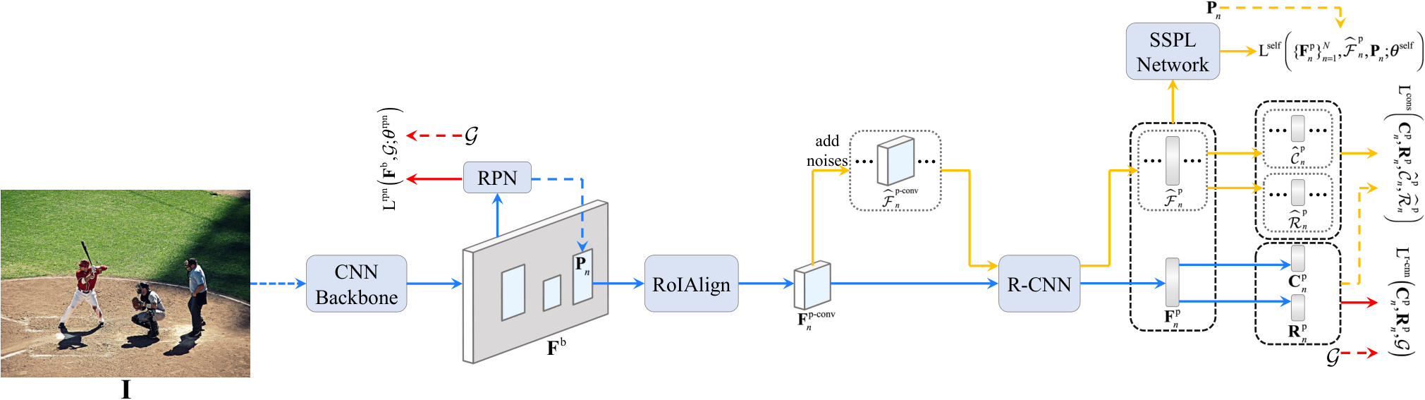
The overall framework of our approach is shown in Fig. 2. As in standard proposal-based object detectors lin2017feature; ren2017faster, during the forward process, first, an input image $\mathbf{I}$ is fed into a CNN backbone (e.g., ResNet-50 he2016deep with feature pyramid networks lin2017feature) with parameters $\bm{\theta}^{\text{b}}$, which produces image convolutional feature maps $\mathbf{F}^{\text{b}}(\mathbf{I};\bm{\theta}^{\text{b}})$. Then, a Region Proposal Network (RPN) with parameters $\bm{\theta}^{\text{rpn}}$ takes $\mathbf{F}^{\text{b}}(\mathbf{I};\bm{\theta}^{\text{b}})$ as inputs to generate region proposals $\mathcal{P}\left(\mathbf{F}^{\text{b}}(\mathbf{I};\bm{\theta}^{\text{b}});\bm{\theta}^{\text{rpn}}\right)$. We use $\mathbf{F}^{\text{b}},\mathcal{P}$ later for simplification, dropping the dependence on $\mathbf{I},\bm{\theta}^{\text{b}},\mathbf{F}^{\text{b}},\bm{\theta}^{\text{rpn}}$. Next, an RoIAlign he2017mask layer takes each proposal $\mathbf{P}_{n}=(x_{n},y_{n},w_{n},h_{n})\in\mathcal{P}$ and $\mathbf{F}^{\text{b}}$ as inputs to extract proposal convolutional feature maps $\mathbf{F}^{\text{p-conv}}_{n}$ (simplification of $\mathbf{F}^{\text{p-conv}}(\mathbf{F}^{\text{b}},\mathbf{P}_{n})$, dropping the dependence on $\mathbf{F}^{\text{b}},\mathbf{P}_{n}$), where $(x_{n},y_{n},w_{n},h_{n})$ denotes the location of the $i^{\text{th}}$ proposal $\mathbf{P}_{n}$, $i\in\{1,2,...,N\}$, and $N$ is the number of proposals in $\mathcal{P}$. After that, $\mathbf{F}^{\text{p-conv}}_{n}$ is fed into a Region-based CNN (R-CNN) to generate proposal features $\mathbf{F}^{\text{p}}(\mathbf{F}^{\text{p-conv}}_{n};\bm{\theta}^{\text{r-cnn}})$ and predictions (i.e., bounding box classification predictions $\mathbf{C}^{\text{p}}\left(\mathbf{F}^{\text{p}}(\mathbf{F}^{\text{p-conv}}_{n};\bm{\theta}^{\text{r-cnn}});\bm{\theta}^{\text{cls}}\right)$ and bounding box regression predictions $\mathbf{R}^{\text{p}}\left(\mathbf{F}^{\text{p}}(\mathbf{F}^{\text{p-conv}}_{n};\bm{\theta}^{\text{r-cnn}});\bm{\theta}^{\text{reg}}\right)$), where $\bm{\theta}^{\text{r-cnn}},\bm{\theta}^{\text{cls}}$, and $\bm{\theta}^{\text{reg}}$ denote parameters of the R-CNN to generate proposal features, bounding box classification predictions, and bounding box regression predictions, respectively. We use $\mathbf{F}^{\text{p}}_{n},\mathbf{C}^{\text{p}}_{n},\mathbf{R}^{\text{p}}_{n}$ later for simplification, dropping the dependence on $\mathbf{F}^{\text{p-conv}}_{n},\bm{\theta}^{\text{r-cnn}},\mathbf{F}^{\text{p}}_{n},\bm{\theta}^{\text{cls}},\bm{\theta}^{\text{reg}}$.

For each labeled data $(\mathbf{I},\mathcal{G})\in\mathcal{D}^{\text{l}}$, it is straightforward to train object detectors according to the standard fully-supervised learning loss defined in Eq. (1), where the first and second terms denote the RPN loss and R-CNN loss respectively. This loss is optimized w.r.t. $\bm{\theta}^{\text{b}},\bm{\theta}^{\text{rpn}},\bm{\theta}^{\text{r-cnn}},\bm{\theta}^{\text{cls}},\bm{\theta}^{\text{reg}}$ to train object detectors during the back-propagation process. More details of the loss function can be found in ren2017faster.

However, for unlabeled data $\mathbf{I}\in\mathcal{D}^{\text{u}}$, there is no available ground truth labels $\mathcal{G}$. Thus we cannot use Eq. (1) to train object detectors on $\mathcal{D}^{\text{u}}$. To train object detectors also on $\mathcal{D}^{\text{u}}$, we present a proposal learning approach, consisting of a self-supervised proposal learning module and a consistency-based proposal learning module, to also learn proposal features (i.e., $\mathbf{F}^{\text{p}}_{n}$) and predictions (i.e., $\mathbf{C}^{\text{p}}_{n},\mathbf{R}^{\text{p}}_{n}$) from $\mathcal{D}^{\text{u}}$. It is possible to also benefit RPN from $\mathcal{D}^{\text{u}}$. We only focus on the R-CNN-related parts, because 1) the final object detection results are from R-CNN-related parts and thus improving the R-CNN-related parts will benefit object detectors directly; 2) gradients will also be back-propagated from the R-CNN-related parts to the CNN backbone to learn better $\mathbf{F}^{b}$, which could potentially improve RPN.

For the $n^{\text{th}}$ proposal $\mathbf{P}_{n}$ of image $\mathbf{I}$, during the forward process, we first generate a set of noisy proposal features $\hat{\mathcal{F}}^{\text{p}}_{n}=\{\hat{\mathbf{F}}^{\text{p}}_{nk}\}_{k=1}^{K}$ and predictions $\hat{\mathcal{C}}^{\text{p}}_{n}=\{\hat{\mathbf{C}}^{\text{p}}_{nk}\}_{k=1}^{K},\hat{\mathcal{R}}^{\text{p}}_{n}=\{\hat{\mathbf{R}}^{\text{p}}_{nk}\}_{k=1}^{K}$, where $K$ denotes the number of noisy proposal features for each $\mathbf{P}_{n}$. As we stated in Section 1, we add noise to proposal features to share convolutional feature computations for the CNN backbone (i.e., $\mathbf{F}^{\text{b}}$) between noisy proposal feature computations and the original proposal feature computations for efficiency. More specifically, we add random noise $\{\epsilon_{nk}\}_{k=1}^{K}$ to proposal convolutional feature maps $\mathbf{F}^{\text{p-conv}}_{n}$, which generates a set of noisy proposal convolutional feature maps $\hat{\mathcal{F}}^{\text{p-conv}}_{n}=\{\hat{\mathbf{F}}^{\text{p-conv}}(\mathbf{F}^{\text{p-conv}}_{n},\epsilon_{nk})\}_{k=1}^{K}$, see Fig. 2. We use $\hat{\mathbf{F}}^{\text{p-conv}}_{nk}$ for simplification, dropping the dependence on $\mathbf{F}^{\text{p-conv}}_{n},\epsilon_{nk}$. Similar to the procedure to generate $\mathbf{F}^{\text{p}}_{n},\mathbf{C}^{\text{p}}_{n},\mathbf{R}^{\text{p}}_{n}$, the noisy proposal feature maps are fed into the R-CNN to generate the noisy proposal features $\hat{\mathcal{F}}^{\text{p}}_{n}=\{\hat{\mathbf{F}}^{\text{p}}_{nk}\}_{k=1}^{K}$ and predictions $\hat{\mathcal{C}}^{\text{p}}_{n}=\{\hat{\mathbf{C}}^{\text{p}}_{nk}\}_{k=1}^{K},\hat{\mathcal{R}}^{\text{p}}_{n}=\{\hat{\mathbf{R}}^{\text{p}}_{nk}\}_{k=1}^{K}$ (we drop the dependence on $\hat{\mathbf{F}}^{\text{p-conv}}_{nk},\bm{\theta}^{\text{r-cnn}},\hat{\mathbf{F}}^{\text{p}}_{nk},\bm{\theta}^{\text{cls}},\bm{\theta}^{\text{reg}}$ for notation simplification).

For Self-Supervised Proposal Learning (SSPL), as shown in Fig. 2, during the forward process, we pass the original proposal features $\mathbf{F}^{\text{p}}_{n}$ and the noisy proposal features $\hat{\mathcal{F}}^{\text{p}}_{n}$ through a small SSPL network with parameters $\bm{\theta}^{\text{self}}$. The outputs of the SSPL network and the proposal location $\mathbf{P}_{n}=(x_{n},y_{n},w_{n},h_{n})$ are taken as inputs to compute SSPL loss $\mathrm{L}^{\text{self}}\left(\{\mathbf{F}^{\text{p}}_{n}\}_{n=1}^{N},\hat{\mathcal{F}}^{\text{p}}_{n},\mathbf{P}_{n};\bm{\theta}^{\text{self}}\right)$ which is defined in later Eq. (6). Since this loss does not take any ground truth labels $\mathcal{G}$ as inputs, by optimizing this loss w.r.t. $\mathbf{F}^{\text{p}}_{n},\hat{\mathcal{F}}^{\text{p}}_{n},\bm{\theta}^{\text{self}}$, i.e., $\bm{\theta}^{\text{b}},\bm{\theta}^{\text{r-cnn}},\bm{\theta}^{\text{self}}$, during the back-propagation process, we can learn proposal features also from unlabeled data. We will give more details about this module in Section 3.3.

For consistency-based proposal learning, as shown in Fig. 2, during the forward process the original proposal predictions $\mathbf{C}^{\text{p}}_{n},\mathbf{R}^{\text{p}}_{n}$ and the noisy proposal predictions $\hat{\mathcal{C}}^{\text{p}}_{n},\hat{\mathcal{R}}^{\text{p}}_{n}$ are taken as inputs to compute loss $\mathrm{L}^{\text{cons}}\left(\mathbf{C}^{\text{p}}_{n},\mathbf{R}^{\text{p}}_{n},\hat{\mathcal{C}}^{\text{p}}_{n},\hat{\mathcal{R}}^{\text{p}}_{n}\right)$ which is defined in later Eq. (9). Following miyato2018virtual; xie2019unsupervised, this loss is optimized w.r.t. $\hat{\mathcal{C}}^{\text{p}}_{n},\hat{\mathcal{R}}^{\text{p}}_{n}$ (not w.r.t. $\mathbf{C}^{\text{p}}_{n},\mathbf{R}^{\text{p}}_{n}$), i.e., $\bm{\theta}^{\text{b}},\bm{\theta}^{\text{r-cnn}},\bm{\theta}^{\text{cls}},\bm{\theta}^{\text{reg}}$, during the back-propagation process. Computing this loss does not require any ground truth labels $\mathcal{G}$, and thus we can learn proposal features and predictions also from unlabeled data. We will give more details about this module in Section 3.4.

We apply the standard fully-supervised loss defined in Eq. (1) to labeled data $\mathcal{D}^{\text{l}}$, and the self-supervised proposal learning loss $\mathrm{L}^{\text{self}}\left(\{\mathbf{F}^{\text{p}}_{n}\}_{n=1}^{N},\hat{\mathcal{F}}^{\text{p}}_{n},\mathbf{P}_{n};\bm{\theta}^{\text{self}}\right)$ and the consistency-based proposal learning loss $\mathrm{L}^{\text{cons}}\left(\mathbf{C}^{\text{p}}_{n},\mathbf{R}^{\text{p}}_{n},\hat{\mathcal{C}}^{\text{p}}_{n},\hat{\mathcal{R}}^{\text{p}}_{n}\right)$ to unlabeled data $\mathcal{D}^{\text{u}}$. The object detectors are trained on $\mathcal{D}^{\text{l}},\mathcal{D}^{\text{u}}$ by optimizing the loss Eq. (2) w.r.t. $\bm{\theta}^{\text{b}},\bm{\theta}^{\text{rpn}},\bm{\theta}^{\text{r-cnn}},\bm{\theta}^{\text{cls}},\bm{\theta}^{\text{reg}},\bm{\theta}^{\text{self}}$ during the back-propagation process.

We can also apply the self-supervised and consistency-based proposal learning losses to both labeled and unlabeled data, following the semi-supervised learning works laine2016temporal; miyato2018virtual; zhai2019s4l. Then the overall loss is written as Eq. (3).

During inference, we simply keep the parts of the standard proposal-based object detectors, see the blue arrows in Fig. 2. Therefore, our approach does not bring any extra inference computations.

Previous works have shown that object detectors can benefit from context bell2016inside; divvala2009empirical; hu2018relation; mottaghi2014role and should be noise-robust michaelis2019benchmarking; wang2017fast. Our self-supervised proposal learning module uses a proposal location loss and a contrastive loss to learn context-aware and noise-robust proposal features respectively.

To compute proposal location loss, we use proposal location prediction as the pretext task, inspired by the approach in doersch2015unsupervised. More specifically, we pass $\mathbf{F}^{\text{p}}_{n},\hat{\mathcal{F}}^{\text{p}}_{n}$ through two fully-connected layers with parameters $\bm{\theta}^{\text{self-loc}}$ and a sigmoid layer to compute location predictions $\mathbf{L}^{\text{p}}_{n},\hat{\mathcal{L}}^{\text{p}}_{n}=\{\hat{\mathbf{L}}^{\text{p}}_{nk}\}_{k=1}^{K}$, where the numbers of the outputs of the two fully-connected layers are $1024$ and $4$ respectively. Here we drop the dependence on $\mathbf{F}^{\text{p}}_{n},\hat{\mathcal{F}}^{\text{p}}_{n},\bm{\theta}^{\text{self-loc}}$ for notation simplification. Then we use $\ell_{2}$ distance to compute proposal location loss, see Eq. (4), where $\tilde{\mathbf{P}}_{n}=(x_{n}/W,y_{n}/H,w_{n}/W,h_{n}/H)$ is a normalized version of $\mathbf{P}_{n}$, and $W,H$ denote the width and height of image $\mathbf{I}$ respectively.

By optimizing this loss w.r.t. $\mathbf{F}^{\text{p}}_{n},\hat{\mathcal{F}}^{\text{p}}_{n},\bm{\theta}^{\text{self-loc}}$, i.e., $\bm{\theta}^{\text{b}},\bm{\theta}^{\text{r-cnn}},\bm{\theta}^{\text{self-loc}}$, we can learn context-aware proposal features because predicting proposal location in an image requires proposal features understanding some global information of the image. We do not use the relative patch location prediction task doersch2015unsupervised directly, because images are large and there are always multiple objects in the same image for object detection, which makes relative patch location prediction hard to be solved.

To compute contrastive loss, we use instance discrimination as the pretext task, following he2019momentum; wu2018unsupervised; ye2019unsupervised. More specifically, we first use a fully-connected layer with parameters $\bm{\theta}^{\text{self-cont}}$ and an $\ell_{2}$ normalization layer to project $\mathbf{F}^{\text{p}}_{n},\hat{\mathcal{F}}^{\text{p}}_{n}$ to embedded proposal features $\mathbf{F}^{\text{embed}}_{n},\hat{\mathcal{F}}^{\text{embed}}_{n}=\{\hat{\mathbf{F}}^{\text{embed}}_{nk}\}_{k=1}^{K}$ (dropping the dependence on $\mathbf{F}^{\text{p}}_{n},\hat{\mathcal{F}}^{\text{p}}_{n},\bm{\theta}^{\text{self-cont}}$), where the numbers of the outputs of the fully-connected layer is $128$. Then the contrastive loss is written as Eq. (5), where $\tau$ is a temperature hyper-parameter.

By optimizing this loss w.r.t. $\mathbf{F}^{\text{p}}_{n},\hat{\mathcal{F}}^{\text{p}}_{n},\bm{\theta}^{\text{self-cont}}$, i.e., $\bm{\theta}^{\text{b}},\bm{\theta}^{\text{r-cnn}},\bm{\theta}^{\text{self-cont}}$, noisy proposal features are enforced to be closer to their original proposal features than to other proposal features, which learns noise-robust proposal features and thus learns noise-robust object detectors.

By combining the proposal location loss in Eq. (4) and the contrastive loss in Eq. (5), the overall self-supervised proposal learning loss is written as Eq. (6), where $\lambda^{\text{self-loc}},\lambda^{\text{self-cont}}$ are loss weights and $\bm{\theta}^{\text{self}}=\{\bm{\theta}^{\text{self-loc}},\bm{\theta}^{\text{self-cont}}\}$. This loss is optimized w.r.t. $\bm{\theta}^{\text{b}},\bm{\theta}^{\text{r-cnn}},\bm{\theta}^{\text{self}}$ to learn proposal features.

To further train noise-robust object detectors, we apply consistency losses miyato2018virtual; sajjadi2016regularization; xie2019unsupervised to ensure consistency between noisy proposal predictions and their original proposal predictions. More precisely, we apply consistency losses to both bounding box classification and regression predictions.

For consistency loss for bounding box classification predictions $\mathbf{C}^{\text{p}}_{n},\hat{\mathcal{C}}^{\text{p}}_{n}$, we use KL divergence as the loss to enforce class predictions from noisy proposals and their original proposals to be consistent, follwing miyato2018virtual; xie2019unsupervised, see Eq. (7).

Unlike image classification containing only classification results, object detection also predicts object locations. To further ensure proposal prediction consistency, we compute consistency loss in Eq. (8) to enforce object location predictions from noisy proposals and their original proposals to be consistent. Here we use the standard bounding box regression loss, i.e., smoothed $\ell_{1}$ loss girshick2015fast. We only selected the easiest noisy proposal feature to compute this loss for training stability.

By combining the consistency losses for bounding box classification predictions in Eq. (7) and for bounding box regression predictions in Eq. (8), the overall consistency-based proposal learning loss is written as Eq. (9), where $\lambda^{\text{cons-cls}},\lambda^{\text{cons-reg}}$ are loss weights. Following miyato2018virtual; xie2019unsupervised, this loss is optimized w.r.t. $\hat{\mathcal{C}}^{\text{p}}_{n},\hat{\mathcal{R}}^{\text{p}}_{n}$ (not w.r.t. $\mathbf{C}^{\text{p}}_{n},\mathbf{R}^{\text{p}}_{n}$), i.e., $\bm{\theta}^{\text{b}},\bm{\theta}^{\text{r-cnn}},\bm{\theta}^{\text{cls}},\bm{\theta}^{\text{reg}}$. Then we can learn more noisy-robust proposal features and predictions.

In this part, we conduct elaborate experiments to analyze the influence of different components of our proposal learning approach, including different losses defined in Eq. (4), (5), (7), (8), applying proposal learning for labeled data, and Fast Stochastic Weight Averaging (FSWA). Without loss of generality, we only use ResNet-50 as our CNN backbone. For the first two subparts, we only apply proposal learning to unlabeled data, i.e., using Eq. (2). For the first three subparts, we do not use FSWA. Results are shown in Table 1, where the first row reports results from fully-supervised baseline, i.e., training object detectors only on labeled data using Eq. (1). For all experiments, we fix the initial random seed during training to ensure that the performance gains come from our approach instead of randomness.

According to these results, in the rest of our paper, we use all components of our proposal learning on both labeled and unlabeled data (i.e., using Eq. (3)), and apply FSWA to our approach.

We report the result comparisons among fully-supervised baselines, Data Distillation (DD) radosavovic2018data, and our approach in Table 2 on the COCO test-dev2017 set. As we can see, our approach obtains consistently better results compared to the fully-supervised baselines for different CNN backbones. In addition, both DD and our approach obtain higher APs than the fully-supervised baselines, which demonstrates that training object detectors on both labeled and unlabeled data outperforms training object detectors only on labeled data, confirming the potentials of semi-supervised object detection. Using our approach alone obtains comparable APs compared to DD.

In particular, we also evaluate the efficiency of our method by combining with DD. More specifically, we first train object detectors using our approach, then follow DD to label unlabeled data, and finally re-train object detectors using both fully-supervised loss and proposal learning losses. The combination of our approach and DD obtains 39.6% (ResNet-50), 41.3% (ResNet-101), 42.8% (ResNeXt-101-32$\times$4d), and 46.2% (ResNeXt-101-32$\times$4d+DCN) APs, which outperforms the fully-supervised baselines by about 2.0% on average and DD alone by 0.9% on average. The results demonstrate that our approach and DD are complementary to some extent.

References

- (1) Ben Athiwaratkun, Marc Finzi, Pavel Izmailov, and Andrew Gordon Wilson. There are many consistent explanations of unlabeled data: Why you should average. arXiv preprint arXiv:1806.05594, 2018.
- (2) Sean Bell, C Lawrence Zitnick, Kavita Bala, and Ross Girshick. Inside-outside net: Detecting objects in context with skip pooling and recurrent neural networks. In Proceedings of the IEEE conference on computer vision and pattern recognition, pages 2874–2883, 2016.
- (3) Avrim Blum and Tom Mitchell. Combining labeled and unlabeled data with co-training. In Proceedings of the eleventh annual conference on Computational learning theory, pages 92–100, 1998.
- (4) Zhaowei Cai and Nuno Vasconcelos. Cascade R-CNN: Delving into high quality object detection. In Proceedings of the IEEE conference on computer vision and pattern recognition, pages 6154–6162, 2018.
- (5) Olivier Chapelle, Bernhard Schlkopf, and Alexander Zien. Semi-supervised learning. 2010.
- (6) Kai Chen, Jiaqi Wang, Jiangmiao Pang, Yuhang Cao, Yu Xiong, Xiaoxiao Li, Shuyang Sun, Wansen Feng, Ziwei Liu, Jiarui Xu, et al. MMDetection: Open MMLab detection toolbox and benchmark. arXiv preprint arXiv:1906.07155, 2019.
- (7) Ramazan Gokberk Cinbis, Jakob Verbeek, and Cordelia Schmid. Weakly supervised object localization with multi-fold multiple instance learning. IEEE transactions on pattern analysis and machine intelligence, 39(1):189–203, 2016.
- (8) Santosh K Divvala, Derek Hoiem, James H Hays, Alexei A Efros, and Martial Hebert. An empirical study of context in object detection. In Proceedings of the IEEE conference on computer vision and pattern recognition, pages 1271–1278, 2009.
- (9) Carl Doersch, Abhinav Gupta, and Alexei A Efros. Unsupervised visual representation learning by context prediction. In Proceedings of the IEEE international conference on computer vision, pages 1422–1430, 2015.
- (10) Mark Everingham, SM Ali Eslami, Luc Van Gool, Christopher KI Williams, John Winn, and Andrew Zisserman. The pascal visual object classes challenge: A retrospective. International journal of computer vision, 111(1):98–136, 2015.
- (11) Jiyang Gao, Jiang Wang, Shengyang Dai, Li-Jia Li, and Ram Nevatia. NOTE-RCNN: Noise tolerant ensemble RCNN for semi-supervised object detection. In Proceedings of the IEEE international conference on computer vision, pages 9508–9517, 2019.
- (12) Golnaz Ghiasi, Tsung-Yi Lin, and Quoc V Le. Dropblock: A regularization method for convolutional networks. In Advances in neural information processing systems, pages 10727–10737, 2018.
- (13) Spyros Gidaris, Praveer Singh, and Nikos Komodakis. Unsupervised representation learning by predicting image rotations. arXiv preprint arXiv:1803.07728, 2018.
- (14) Ross Girshick. Fast R-CNN. In Proceedings of the IEEE international conference on computer vision, pages 1440–1448, 2015.
- (15) Ross Girshick, Jeff Donahue, Trevor Darrell, and Jitendra Malik. Rich feature hierarchies for accurate object detection and semantic segmentation. In Proceedings of the IEEE conference on computer vision and pattern recognition, pages 580–587, 2014.
- (16) Kaiming He, Haoqi Fan, Yuxin Wu, Saining Xie, and Ross Girshick. Momentum contrast for unsupervised visual representation learning. arXiv preprint arXiv:1911.05722, 2019.
- (17) Kaiming He, Georgia Gkioxari, Piotr Dollár, and Ross Girshick. Mask R-CNN. In Proceedings of the IEEE international conference on computer vision, pages 2980–2988, 2017.
- (18) Kaiming He, Xiangyu Zhang, Shaoqing Ren, and Jian Sun. Deep residual learning for image recognition. In Proceedings of the IEEE conference on computer vision and pattern recognition, pages 770–778, 2016.
- (19) Judy Hoffman, Sergio Guadarrama, Eric S Tzeng, Ronghang Hu, Jeff Donahue, Ross Girshick, Trevor Darrell, and Kate Saenko. LSDA: Large scale detection through adaptation. In Advances in Neural Information Processing Systems, pages 3536–3544, 2014.
- (20) Han Hu, Jiayuan Gu, Zheng Zhang, Jifeng Dai, and Yichen Wei. Relation networks for object detection. In Proceedings of the IEEE conference on computer vision and pattern recognition, pages 3588–3597, 2018.
- (21) Zhaojin Huang, Lichao Huang, Yongchao Gong, Chang Huang, and Xinggang Wang. Mask scoring R-CNN. In Proceedings of the IEEE conference on computer vision and pattern recognition, pages 6409–6418, 2019.
- (22) Jisoo Jeong, Seungeui Lee, Jeesoo Kim, and Nojun Kwak. Consistency-based semi-supervised learning for object detection. In Advances in neural information processing systems, pages 10758–10767, 2019.
- (23) Longlong Jing and Yingli Tian. Self-supervised visual feature learning with deep neural networks: A survey. arXiv preprint arXiv:1902.06162, 2019.
- (24) Alexander Kolesnikov, Xiaohua Zhai, and Lucas Beyer. Revisiting self-supervised visual representation learning. In Proceedings of the IEEE conference on computer vision and pattern recognition, pages 1920–1929, 2019.
- (25) Alex Krizhevsky, Ilya Sutskever, and Geoffrey E Hinton. ImageNet classification with deep convolutional neural networks. In Advances in neural information processing systems, pages 1097–1105, 2012.
- (26) Samuli Laine and Timo Aila. Temporal ensembling for semi-supervised learning. arXiv preprint arXiv:1610.02242, 2016.
- (27) Yann LeCun, Léon Bottou, Yoshua Bengio, and Patrick Haffner. Gradient-based learning applied to document recognition. Proceedings of the IEEE, 86(11):2278–2324, 1998.
- (28) Tsung-Yi Lin, Piotr Dollár, Ross Girshick, Kaiming He, Bharath Hariharan, and Serge Belongie. Feature pyramid networks for object detection. In Proceedings of the IEEE conference on computer vision and pattern recognition, pages 2117–2125, 2017.
- (29) Tsung-Yi Lin, Priyal Goyal, Ross Girshick, Kaiming He, and Piotr Dollár. Focal loss for dense object detection. IEEE transactions on pattern analysis and machine intelligence, 2018.
- (30) Tsung-Yi Lin, Michael Maire, Serge Belongie, James Hays, Pietro Perona, Deva Ramanan, Piotr Dollár, and C Lawrence Zitnick. Microsoft COCO: Common objects in context. In European conference on computer vision, pages 740–755, 2014.
- (31) Wei Liu, Dragomir Anguelov, Dumitru Erhan, Christian Szegedy, Scott Reed, Cheng-Yang Fu, and Alexander C Berg. SSD: Single shot multibox detector. In European conference on computer vision, pages 21–37, 2016.
- (32) Claudio Michaelis, Benjamin Mitzkus, Robert Geirhos, Evgenia Rusak, Oliver Bringmann, Alexander S Ecker, Matthias Bethge, and Wieland Brendel. Benchmarking robustness in object detection: Autonomous driving when winter is coming. arXiv preprint arXiv:1907.07484, 2019.
- (33) Takeru Miyato, Shin-ichi Maeda, Masanori Koyama, and Shin Ishii. Virtual adversarial training: a regularization method for supervised and semi-supervised learning. IEEE transactions on pattern analysis and machine intelligence, 41(8):1979–1993, 2018.
- (34) Roozbeh Mottaghi, Xianjie Chen, Xiaobai Liu, Nam-Gyu Cho, Seong-Whan Lee, Sanja Fidler, Raquel Urtasun, and Alan Yuille. The role of context for object detection and semantic segmentation in the wild. In Proceedings of the IEEE conference on computer vision and pattern recognition, pages 891–898, 2014.
- (35) Adam Paszke, Sam Gross, Francisco Massa, Adam Lerer, James Bradbury, Gregory Chanan, Trevor Killeen, Zeming Lin, Natalia Gimelshein, Luca Antiga, et al. PyTorch: An imperative style, high-performance deep learning library. In Advances in neural information processing systems, pages 8024–8035, 2019.
- (36) Deepak Pathak, Philipp Krahenbuhl, Jeff Donahue, Trevor Darrell, and Alexei A Efros. Context encoders: Feature learning by inpainting. In Proceedings of the IEEE conference on computer vision and pattern recognition, pages 2536–2544, 2016.
- (37) Siyuan Qiao, Wei Shen, Zhishuai Zhang, Bo Wang, and Alan Yuille. Deep co-training for semi-supervised image recognition. In European conference on computer vision, pages 135–152, 2018.
- (38) Ilija Radosavovic, Piotr Dollár, Ross Girshick, Georgia Gkioxari, and Kaiming He. Data distillation: Towards omni-supervised learning. In Proceedings of the IEEE conference on computer vision and pattern recognition, pages 4119–4128, 2018.
- (39) Joseph Redmon, Santosh Divvala, Ross Girshick, and Ali Farhadi. You only look once: Unified, real-time object detection. In Proceedings of the IEEE conference on computer vision and pattern recognition, pages 779–788, 2016.
- (40) Shaoqing Ren, Kaiming He, Ross Girshick, and Jian Sun. Faster R-CNN: Towards real-time object detection with region proposal networks. IEEE transactions on pattern analysis and machine intelligence, 39(6):1137–1149, 2017.
- (41) Olga Russakovsky, Jia Deng, Hao Su, Jonathan Krause, Sanjeev Satheesh, Sean Ma, Zhiheng Huang, Andrej Karpathy, Aditya Khosla, Michael Bernstein, et al. Imagenet large scale visual recognition challenge. International journal of computer vision, 115(3):211–252, 2015.
- (42) Mehdi Sajjadi, Mehran Javanmardi, and Tolga Tasdizen. Regularization with stochastic transformations and perturbations for deep semi-supervised learning. In Advances in neural information processing systems, pages 1163–1171, 2016.
- (43) Shuai Shao, Zeming Li, Tianyuan Zhang, Chao Peng, Gang Yu, Xiangyu Zhang, Jing Li, and Jian Sun. Objects365: A large-scale, high-quality dataset for object detection. In Proceedings of the IEEE international conference on computer vision, pages 8430–8439, 2019.
- (44) Peng Tang, Chunyu Wang, Xinggang Wang, Wenyu Liu, Wenjun Zeng, and Jingdong Wang. Object detection in videos by high quality object linking. IEEE transactions on pattern analysis and machine intelligence, 2019.
- (45) Yuxing Tang, Josiah Wang, Boyang Gao, Emmanuel Dellandréa, Robert Gaizauskas, and Liming Chen. Large scale semi-supervised object detection using visual and semantic knowledge transfer. In Proceedings of the IEEE conference on computer vision and pattern recognition, pages 2119–2128, 2016.
- (46) Antti Tarvainen and Harri Valpola. Mean teachers are better role models: Weight-averaged consistency targets improve semi-supervised deep learning results. In Advances in neural information processing systems, pages 1195–1204, 2017.
- (47) Jonathan Tompson, Ross Goroshin, Arjun Jain, Yann LeCun, and Christoph Bregler. Efficient object localization using convolutional networks. In Proceedings of the IEEE conference on computer vision and pattern recognition, pages 648–656, 2015.
- (48) Jingdong Wang, Ke Sun, Tianheng Cheng, Borui Jiang, Chaorui Deng, Yang Zhao, Dong Liu, Yadong Mu, Mingkui Tan, Xinggang Wang, Wenyu Liu, and Bin Xiao. Deep high-resolution representation learning for visual recognition. arXiv preprint arXiv:1908.07919, 2019.
- (49) Xiaolong Wang, Abhinav Shrivastava, and Abhinav Gupta. A-Fast-RCNN: Hard positive generation via adversary for object detection. In Proceedings of the IEEE Conference on computer vision and pattern recognition, pages 2606–2615, 2017.
- (50) Zhirong Wu, Yuanjun Xiong, Stella X Yu, and Dahua Lin. Unsupervised feature learning via non-parametric instance discrimination. In Proceedings of the IEEE conference on computer vision and pattern recognition, pages 3733–3742, 2018.
- (51) Qizhe Xie, Zihang Dai, Eduard Hovy, Minh-Thang Luong, and Quoc V Le. Unsupervised data augmentation. arXiv preprint arXiv:1904.12848, 2019.
- (52) Saining Xie, Ross Girshick, Piotr Dollár, Zhuowen Tu, and Kaiming He. Aggregated residual transformations for deep neural networks. In Proceedings of the IEEE conference on computer vision and pattern recognition, pages 1492–1500, 2017.
- (53) David Yarowsky. Unsupervised word sense disambiguation rivaling supervised methods. In Proceedings of the 33rd annual meeting of the association for computational linguistics, pages 189–196, 1995.
- (54) Mang Ye, Xu Zhang, Pong C Yuen, and Shih-Fu Chang. Unsupervised embedding learning via invariant and spreading instance feature. In Proceedings of the IEEE Conference on computer vision and pattern recognition, pages 6210–6219, 2019.
- (55) Xiaohua Zhai, Avital Oliver, Alexander Kolesnikov, and Lucas Beyer. S4L: Self-supervised semi-supervised learning. In Proceedings of the IEEE international conference on computer vision, pages 1476–1485, 2019.
- (56) Richard Zhang, Phillip Isola, and Alexei A Efros. Colorful image colorization. In European conference on computer vision, pages 649–666, 2016.
- (57) Zhishuai Zhang, Siyuan Qiao, Cihang Xie, Wei Shen, Bo Wang, and Alan L Yuille. Single-shot object detection with enriched semantics. In Proceedings of the IEEE conference on computer vision and pattern recognition, pages 5813–5821, 2018.
- (58) Yuyin Zhou, Yan Wang, Peng Tang, Song Bai, Wei Shen, Elliot Fishman, and Alan Yuille. Semi-supervised 3D abdominal multi-organ segmentation via deep multi-planar co-training. In IEEE winter conference on applications of computer vision, pages 121–140, 2019.
- (59) Xiaojin Zhu and Zoubin Ghahramani. Learning from labeled and unlabeled data with label propagation. 2002.
- (60) Xizhou Zhu, Han Hu, Stephen Lin, and Jifeng Dai. Deformable ConvNets v2: More deformable, better results. In Proceedings of the IEEE conference on computer vision and pattern recognition, pages 9308–9316, 2019.