Non-Hermitian band topology and skin modes in active elastic media

Here we place elasticity within the broader context of non-Hermitian continuum mechanics. We start from the following generic linear momentum conservation equation for a viscoelastic medium:

where $u_{i}(\mathbf{x})$ is the displacement field and $\rho$ is the mass density. The right-hand side of Eq. (S1) divides the total force density into two contributions: the divergence of the stress tensor $\partial_{i}\sigma_{ij}$ captures the internal forces that a solid exerts on itself without requiring contact with an external medium, while $f^{b}_{i}$ captures interactions that require contact with an external medium to supply linear momentum.

Significant attention has been given to the role of $f^{b}_{i}$ in non-Hermitian solids. A few examples include terms of the following form:

The first term $\Gamma_{ij}\dot{u}_{j}$, for example, has been linked to symmetry protected exceptional rings in the context of Coriolis forces, substrate drag, and magnetic fields benzoni2020; Yoshida2019cl. The second term, $K_{ij}u_{j}$, generically arises in systems with pinning Nash2015; Wang2015. Finally, the third term, $K_{ijk}\partial_{j}u_{k}$ arises naturally in systems that contain effective pairwise interactions that violate Newton’s third law Beatus2006; Brandenbourger2019; Rosa2020; Zhou2020; Ghatak2019Realization. It has been shown that this term can give rise to the non-Hermitian skin effect Rosa2020; Zhou2020; Ghatak2019Realization. In these cases, background mechanisms, such as robotic actuators Ghatak2019Realization or rotor systems Zhou2020, provide a linear momentum bias that intuitively localizes all the vibrational modes to one side of the system.

It is intriguing to ask: what are the consequences of internal forces that are non-Hermitian yet respect linear momentum conservation? These contributions arise from $\sigma_{ij}$, and can be decomposed as

Here, $\sigma_{ij}^{\text{int}}$ are the stresses that arise due to internal degrees of freedom, such as nematic Prost2015; Souslov2017 or piezoelectric White1962 stresses. By contrast, $\sigma_{ij}^{u}$ are stresses due to geometric deformations. In the limit of a low Deborah number Lakes2009, one can generically write these terms as

The second term, $\eta_{ijmn}$, is the viscosity tensor, and it couples to the rate of deformation. Materials with broken time reversal symmetry can exhibit a dissipationless odd (or Hall) viscosity $\eta_{ijmn}^{o}=-\eta^{o}_{mnij}$, extensively explored in the context of fluids Banerjee2017; Han2020; Souslov2020PRE; Wiegmann2014; Soni2018; Avron1998; Sone2019; Sone2019arxiv.

However, the first term $C_{ijmn}$ is the elastic modulus tensor and couples only to the static strain. In active systems, $C_{ijmn}$ can acquire an antisymmetric (or odd) part $C^{o}_{ijmn}=-C^{o}_{mnij}$, which introduces non-Hermiticity into the equations of motion Scheibner2020. The elasticity is the unique term that does not require external sources of linear momentum, rate-dependent forces, or auxiliary internal degrees of freedom. Hence, the conceptual limit of a purely elastic solid provides insight into the role played by non-Hermiticity in the relationship between stress and static deformation.

Here, we show how the presence of $C^{o}_{ijmn}$ in conjunction with anisotropy can give rise to the non-Hermitian skin effect. Specifically, we consider the effect of $C^{o}_{ijmn}$ on the spectrum of the operator $D_{in}=C_{ijmn}\partial_{j}\partial_{m}$. We will work in two dimensions, for which it is useful to introduce the following basis of $2\times 2$ matrices:

Using this basis, we can represent $C_{ijmn}$ as a $4\times 4$ matrix:

Notice that the operation $C^{\alpha\beta}\mapsto C^{\beta\alpha}$ corresponds to $C_{ijmn}=C_{mnij}$. Hence, introducing antisymmetry into the matrix $C^{\alpha\beta}$ indicates that the solid’s elastic response does not derive from a potential energy. Furthermore, one can impose the requirements $C^{1\alpha}=0$, which implies that the solid does not have an internal source of angular momentum, and $C^{\alpha 1}=0$, which implies that solid-body rotations do not induce stress Scheibner2020. While metamaterials can violate these properties Lakes2001; Lakes2016; Banerjee2017, they are not necessary ingredients for the non-Hermitian skin effect. In the main text, we consider a solid with the following moduli:

Notice that the modulus $G^{o}$ violates the symmetry of $C^{\alpha\beta}$, and therefore the major symmetry of the tensor $C_{ijmn}$. The modulus $\mu$ is the standard isotropic shear modulus. In the main text, we omit the second row and second column of Eq. (S10) as they are entirely zero. In standard tensor notation, we have:

Working in reciprocal space, the operator $\hat{D}$ may be written as the following matrix:

where $q^{2}=q_{x}^{2}+q_{y}^{2}$. We find that $\hat{D}$ has the following eigenvalues:

Notice that the spectrum does not retrace itself in the complex plane as a function of $q_{x}$ at constant $q_{y}$ (cf. main-text Fig. 1). Hence, when a boundary is introduced parallel to the $y$-axis, no two Bloch modes are able to interfere to satisfy the given boundary conditions (such as displacement- or stress-free). Yet, even in the presence of a boundary, the system still has approximate translational symmetry, so modes with spatial variation of the form $e^{ixq_{x}}e^{-\kappa x}$ are candidates for approximate solutions. As illustrated by Fig. 1c, introducing nonzero $\kappa$ and analytically continuing $\hat{D}(\mathbf{q})$ restores the spectral degeneracies necessary to satisfy the system’s boundary conditions.

Finally, we note that the skin effect is sensitive to the angle of the boundary. For example, if the boundary is rotated $45^{\circ}$, then the spectrum becomes:

where $q_{\parallel}$ ($q_{\perp}$) are parallel (perpendicular) to the boundary. Notice that Eq. (S14) is even under $q_{\perp}\mapsto-q_{\perp}$, thereby suppressing the skin effect.

In the main text, we present the interaction:

where $\mathbf{\hat{r}}$ ($\boldsymbol{\hat{\phi}}$) is a unit vector pointing along (transverse to) the bond vector, $\delta r$ is the change in length of the bond, and $k$ and $k^{a}$ are the passive and active spring constants, respectively. Equivalently, we may express this force law as:

where $k^{t}=\sqrt{k^{2}+(k^{a})^{2}}$ is the stiffness, $\hat{\mathbf{n}}_{\theta}$ is the unit vector rotated by an angle $\theta=\arctan(k^a/k)$ with respect to the bond vector, and $\delta r=r-r_{0}$ is the displacement from its equilibrium separation $r_{0}$, see Fig. 2a of the main text. As a matrix, we may write Eq. (S15) as:

where $\mathbf{u}=\mathbf{r}-\mathbf{r}_{0}$ is the displacement of the bond vector $\mathbf{r}$ from its rest configuration $\mathbf{r}_{0}$. We note that the $k^{a}$ violates the symmetry of the matrix in Eq. (S17), and hence violates Maxwell-Betti reciprocity at the level of a single bond. Here, we show that Eq. (S15) is the most general 2D pairwise interaction obeying the following conditions:

1. (i)

   The interaction only depends on the distance between the particles.

2. (ii)

   The interaction conserves linear momentum.

3. (iii)

   The interaction is linear in its displacements from an equilibrium length $r_{0}$.

For a 2D interaction obeying property (i), it is sufficient to specify the forces $\mathbf{F}_{1}(r)$ and $\mathbf{F}_{2}(r)$ on the two participating particles as a function of their separation $r$. Condition (ii) implies that $\mathbf{F}_{1}(r)=-\mathbf{F}_{2}(r)$, so we need only specify a single function $\mathbf{F}(r)$. By assumption (iii), we may write $\mathbf{F}(r)=-\mathbf{k}\delta r$, where $\mathbf{k}$ is a 2D vector and $\delta r=r-r_{0}$ is the displacement from mechanical equilibrium. By parameterizing $\mathbf{k}$ as $\mathbf{k}=k^{t}\hat{\mathbf{n}}_{\theta}$, we obtain Eq. (S16).

We will often interpret our results in the context of an overdamped equation of motion: $\Gamma\partial_{t}\mathbf{u}=\mathbf{F}$, which reads:

With these dynamics, the conditions of dynamic stability of a single spring is:

Assuming without loss of generality that $\Gamma,k^{t}>0$, the system is stable for $\theta\in[-\pi/2,\pi/2]$.

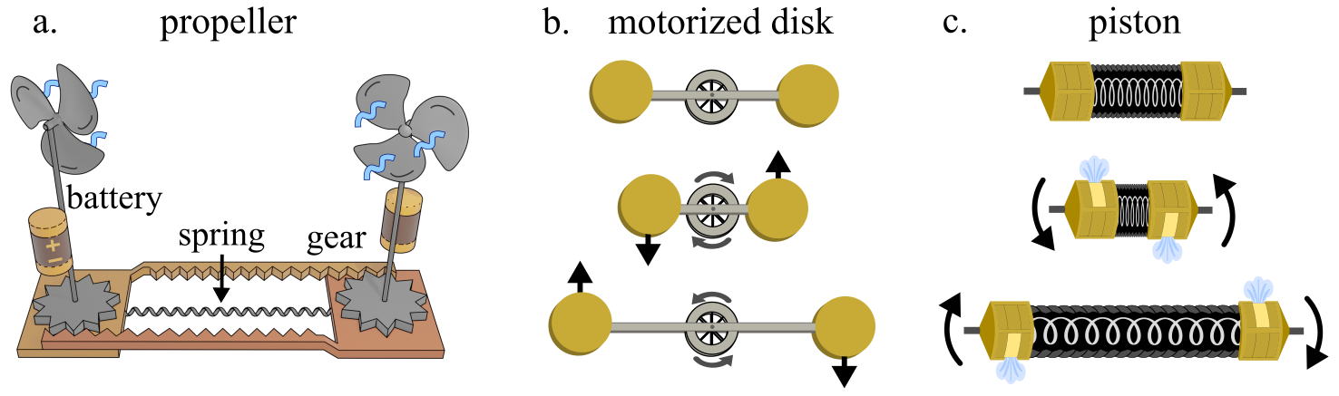
Figure S1 shows three simple mechanical realizations of the active bond adapted from Ref. Scheibner2020. The first example (a) consists of battery powered propellers that blow air at a constant rate. As the mechanism elongates and contracts, a gear system rotates the propellers to produce transverse forces which are proportional to the elongation or contraction for small strains. In example (b), two masses (yellow) are connected by a robotic bond housing an internal motor. As the bond elongates or contracts, the motor accelerates a disk (silver) whose reaction torques are felt by the masses. This example has the intriguing feature that the angular momentum is drawn from a source (i.e. the disk) housed inside the bond rather than a substrate or background fluid. The final example is a system of internally pressurized pistons. When the piston elongates or contracts, vents open to eject the internal fluid and thereby produce a transverse force.

Now we show how Eq. (S18), which describes the overdamped dynamics of a system with active, non-conservative bonds, can be mapped onto the inertial dynamics of a gyroscopic metamaterial with conservative spring-like interactions and weak dissipation. Consider a system of gyroscopes suspended vertically with their bases fixed and free ends connected by Hookean springs, similar to those studied in Refs. Mitchell2018; Mitchell2018Realization; Mitchell2018Nature; Nash2015; Wang2015. In the fast-spinning limit, the angular momentum of the gyroscope is given by $\mathbf{L}=\Omega I{\hat{\boldsymbol{\ell}\mkern 2.0mu}\mkern-2.0mu}{}$, where $\Omega$ and $I$ are, respectively, the angular velocity and moment of inertia about the axis of the gyroscope ${\hat{\boldsymbol{\ell}\mkern 2.0mu}\mkern-2.0mu}{}$. When a force $\mathbf{F}$ is applied to the free tip, the gyroscope experiences a torque

about its fixed base, where $\ell$ is the length of the gyroscope. We have assumed for simplicity that the center of mass of the gyroscope coincides with the point at which the force acts. Hence, we obtain the equation of motion:

We will now use a Cartesian coordinate system in which $\hat{\bf z}$ is oriented vertically, parallel to the rest orientation of the gyroscopes. For small deflections from vertical, we may write the in-plane displacements of each gyroscope’s tip as $u_{x}=\ell\hat{\ell}_{x}$ and $u_{y}=\ell\hat{\ell}_{y}$. When two gyroscopes are connected by Hookean springs, such that the spring is at its rest length $r_{0}$ when the gyroscopes are vertical, the in-plane spring forces are given by:

to leading order in $u_{i}$. In Eq. (S24), the index $i$ runs over $x$ and $y$, $\hat{n}_{i}$ is the in-plane bond vector, and $\delta r=r-r_{0}$ is the change in spring length. We note that geometric nonlinearities, such as out-of-plane motion of the spring, are subleading in $u_{i}$.

In addition to the spring force, we consider a dissipative drag term that takes the form:

Combining Eqs. (S23-S25), the in-plane equations of motion to leading order in $u_{i}$ become:

Now we define

We note that $\hat{n}_{\theta i}$ in Eq. (S28) is simply the vector $\hat{n}_{i}$ rotated through the angle $\theta=\arctan( \frac{\Omega I}{\gamma\ell} )$. Using the definitions of $\Gamma$ and $\hat{n}_{\theta i}$, Eq. (S26) takes the form:

which is mathematically identical in form to Eq. (S18). Notice, however, that Eq. (S29) describes a system of gyroscopes with conservative interactions and weak dissipation. While Eq. (S29) is mathematically equivalent to Eq. (S18), the righthand side of Eq. (S29) should not be interpreted as a physical force. Rather, the righthand side is a subset of the total torque that governs the evolution of the angular momentum parameterized by $u_{i}$. We note that when the dissipation vanishes, $\gamma=0$, equation Eq. (S29) goes to the $\theta=\pi/2$ limit and describes a system for which energy is conserved.

Here, we clarify our definitions and notation regarding $\mathcal{PT}$ symmetry ashida2020; Mostafazadeh2015; Bernard2002; Bender1998. Given a matrix $H$, we say that $H$ is $\mathcal{PT}$ symmetric if there exists an anti-unitary operator $\mathcal{PT}$ with $(\mathcal{PT})^{2}=1$ such that $\commutator{\PT}{H}=0$. We note that $\mathcal{PT}$ symmetry implies that all the eigenvalues of $H$ are either real or come in complex conjugate pairs. To see this, suppose $\mathbf{u}$ is an eigenvector of $H$ with eigenvalue $\lambda$, and let $\mathbf{v}=\mathcal{PT}\mathbf{u}$. Then we have

Hence, $\mathbf{v}$ is an eigenvector of $H$ with eigenvalue $\lambda^{*}$. If all the eigenvalues of $H$ are real, then it is possible to simultaneously diagonalize $H$ and $\mathcal{PT}$. In this case, we say that $H$ is $\mathcal{PT}$-unbroken. If not all the eigenvalues of $H$ are real, we say that $H$ is $\mathcal{PT}$-broken.

The transition between $\mathcal{PT}$-broken and $\mathcal{PT}$-unbroken phases are generically accompanied by exceptional points. To see why, first suppose that $H$ is a function of some parameter $\gamma$ such that an eigenvalue $\lambda$ is real for $\gamma\leq 0$ and complex for $\gamma>0$. At $\gamma=0$, $H$ must experience a spectral degeneracy, since the complex conjugate pairs $\lambda$ and $\lambda^{*}$ in the broken phase must approach each other. For all $\gamma>0$, let $P$ be the projection operator onto the subspace of the eigenvectors $\mathbf{u}$ and $\mathbf{v}$ corresponding to eigenvalues $\lambda$ and $\lambda^{*}$ and related by $\mathbf{v}=\mathcal{PT}\mathbf{u}$. It is easily checked that $\mathcal{PT}P\mathcal{PT}=P$. Hence, $P\mathcal{PT}P$ is a $\mathcal{PT}$ symmetry of $PHP$. Thus, by choosing an appropriate basis on the subspace of $\mathbf{u}$ and $\mathbf{v}$, we may write $P\mathcal{PT}P=\mathcal{K}$. Hence, in this basis, the most general form of $PHP$ as a $2\times 2$ matrix is:

whose eigenvalues are $\lambda_{\pm}=a\pm\sqrt{b^{2}+c^{2}-d^{2}}$ and whose eigenvectors are:

The degeneracy occurs at $d^{2}=c^{2}+b^{2}$, at which point the two eigenvectors $\mathbf{w}_{+}$ and $\mathbf{w}_{-}$ generically coalesce, indicating that $H$ exhibits and exceptional point. However, an exceptional point may be avoided if $H$ is fine tuned such that $b,c,d\to 0$ as $\gamma\to 0$.

Finally, we note that $H$ is $\mathcal{PT}$ symmetric if and only if $H$ is pseudo-Hermitian ashida2020; Mostafazadeh2015. For an invertible matrix $\eta$, we say $H$ is $\eta$-pseudo-Hermitian iff $\eta H\eta^{-1}=H^{\dagger}$. We say that $H$ is pseudo-Hermitian iff there exists an invertible matrix $\eta$ such that $H$ is $\eta$-pseudo-Hermitian. It can be shown that $H$ is $\mathcal{PT}$-unbroken if and only if it is $\eta$-pseudo-Hermitian for some a positive definite invertible matrix $\eta$. Finally, we often refer to instances of $\mathcal{PT}$ symmetry as generalized $\mathcal{PT}$ symmetry to indicate that they do not represent physical notions of time reversal or parity.

In our work, we highlight two primary manifestation of $\mathcal{PT}$ symmetry. The first arises from the fact that the dynamical matrix $D(\mathbf{x},\mathbf{x}^{\prime})$ for a system of $N$ particles is a real $2N\times 2N$ matrix. Hence, $D(\mathbf{x},\mathbf{x}^{\prime})$ commutes with the complex conjugation operator $\mathcal{K}$. Since $\mathcal{K}$ is an anti-unitary operator with $\mathcal{K}^{2}=1$, it satisfies the definition of a (generalized) $\mathcal{PT}$ symmetry. In the language of Hermitian quantum mechanics, this symmetry would typically be referred to as time-reversal symmetry. This notion of $\mathcal{PT}$ symmetry does not rely on details of the network geometry, such as periodic order.

To understand physical significance of the $\mathcal{PT}$-broken and unbroken phases, consider an eigenvalue $\lambda$ with eigenvector $\mathbf{u}(\mathbf{x})$. Let us impose a displacement controlled protocol in which a the eigenvector is actuated in a periodic manner, with the physical displacement given by $\mathbf{d}(\mathbf{x},t)=\real[e^{i\omega_{0}t}\mathbf{u}(\mathbf{x})]$, where $\omega_{0}$ is an external parameter. If $\lambda$ is real, $\mathbf{u}(\mathbf{x})$ may be chosen real. In this case, the trajectory of each particle traces out a straight line $\mathbf{d}(\mathbf{x},t)=\mathbf{u}(\mathbf{x})\cos(w_0 t)$. The work done over the cycle is given by:

Hence, the bonds do zero net work along the cycle. However, if $\lambda=\lambda_{R}+i\lambda_{I}$ is complex, the eigenvector $\mathbf{u}(\mathbf{x})$ must be of the form: $\mathbf{u}(\mathbf{x})=\mathbf{v}(\mathbf{x})+i\mathbf{w}(\mathbf{x})$, where $\mathbf{w}(\mathbf{x})$ and $\mathbf{v}(\mathbf{x})$ are real and may be chosen such that $\sum_{\mathbf{x}}\mathbf{v}(\mathbf{x})\cdot\mathbf{w}(\mathbf{x})=0$. Then the displacement of a single particle traces out open arcs: $\mathbf{d}(x,t)=\mathbf{v}(\mathbf{x})\cos(\omega_0 t)+\mathbf{w}(\mathbf{x})\sin(\omega_0 t).$ Hence, the relative coordinates of the non-potential bonds trace out circles which correspond to energy injected or drawn from their microscopic sources. The total work is given by:

and is manifestly nonzero. Notice that the cycle may be performed quasistically and that reversing the cycle reverses the flow of energy. Operating the cycles at a fixed frequency $\omega_{0}$ merely illustrates the flow of energy. If the system is endowed with a given equation of motion in time, the frequency becomes a function of the eigenvalue $\lambda$. For example, for an overdamped system $\Gamma\partial_{t}\mathbf{u}(\mathbf{x})=\mathbf{F}(\mathbf{x})$, a real $\lambda$ indicates exponential relaxation (Fig. 2e left), while imaginary $\lambda$ indicates circulation (Fig. 2e right) since the energy injection balances the dissipative drag. The connection between $\mathcal{PT}$ symmetry and eigenmodes is also evident in the continuum: when $G^{o}=0$, the displacement field traces out straight lines (Fig. 1d left); and for sufficiently large $G^{o}$, the displacement field traces out ellipses (Fig. 1d center and right).

We now consider networks on periodic lattices, for which we may write the dynamical matrix as a $2n\times 2n$ matrix valued function of wavenumber $D(\mathbf{q})$, where $n$ is the number of particles per unit cell. In this case, the $\mathcal{PT}=\mathcal{K}$ symmetry discussed in the preceding section can be expressed as $D(\mathbf{q})=D^{*}(-\mathbf{q})$. Hence, at a single point in $\mathbf{q}$-space, the $\mathcal{PT}=\mathcal{K}$ symmetry does not constrain the eigenvalues of the $2n\times 2n$ matrix $D(\mathbf{q})$. However, as discussed below, the matrix $D(\mathbf{q})$ itself can become $\mathcal{PT}$ symmetric when additional lattice symmetries are present.

One of the consequences of the is second notion of $\mathcal{PT}$ symmetry is the emergence of symmetry protected exceptional rings (SPERs) Yoshida2019cl; Yoshida2019qu; Okugawa2019; Budich2019. Suppose that $D(\mathbf{q})$ is $\mathcal{PT}$-broken at point $\mathbf{q}_{0}$ and $\mathcal{PT}$-unbroken at point $\mathbf{q}_{1}$. Let $\mathbf{k}_{\alpha}(\gamma)$ a family of homotopically equivalent curves in the Brillouin zone such that $\mathbf{k}_{\alpha}(0)=\mathbf{q}_{0}$ and $\mathbf{k}_{\alpha}(1)=\mathbf{q}_{1}$. For each $\alpha$, there must be at least one point $\gamma^{*}$ such that $D(\mathbf{k}_{\alpha})$ transitions from being $\mathcal{PT}$-broken to $\mathcal{PT}$-unbroken, which generically corresponds to an exceptional point. By continuity, the the quantity $\mathbf{k}^{*}_{\alpha}$, treated as a function of $\alpha$, traces out a 1D curve in the Brillouin zone. Hence, the $\mathcal{PT}$ symmetry induces exceptional rings. If there are several values of $\gamma$ at which $D(\mathbf{q})$ is defective, then there will be several exceptional rings traced out as a function of $\alpha$.

In the main text, we present the example of the honeycomb lattice, whose dynamical matrix $D_{\theta}(\mathbf{q})$ is given in Eq. (S73). The honeycomb lattice has an inversion symmetry such that $UD_{\theta}(-\mathbf{q})U^{-1}=D_{\theta}(\mathbf{q})$, where

Combining the reality condition with the inversion symmetry, we can define the anti-unitary operator $\mathcal{PT}=U\mathcal{K}$. We note that $\commutator{\PT}{D_\theta(\vb q)}=0$ for each point in $\mathbf{q}$ space. In Fig. S2, we show the determinant of the matrix of right eigenvectors $V$ of $D_{\theta}(\mathbf{q})$ over the Brillouin zone. The exceptional rings correspond to zeros of the determinant. When we remove the inversion symmetry, for instance by adding different masses or drag coefficients to the two particles, the exceptional vanish and only exceptional points remain.

In Ref. Yoshida2019cl, SPERSs are observed as a result of an emergent mechanical $\mathcal{CP}$ symmetry. We note that Ref. Yoshida2019cl utilizes an effective Hamiltonian formalism since the non-Hermiticty considered there enters through velocity dependent forces (e.g. Coriolis or drag forces) rather than the displacement-force relationship captured by the the dynamical matrix. While the physical origin of the non-Hermiticity and the mathematical object under consideration differ, our derivations follow closely those presented in Ref. Yoshida2019cl. This parallel arises since a matrix with $\mathcal{PT}$ symmetry can be transformed into one with $\mathcal{CP}$-symmetry through multiplication by $i$ Kawabata2019NatCom.

We now show that violation of $\mathcal{PT}$ symmetry is necessary for a nonzero Chern number. Recall that the Berry curvature associated with the $n$th band of a Hermitian Hamiltonian of a 2D system is given by:

where $A_{j}(\mathbf{q})$ is the Berry connection:

and $\ket{n(\vb q)}$ is the eigenvector associated with the $n$th band FRUCHART2013. For a Hermitian operator $H$, the eigenvector $\ket{n(\vb q)}$ obeys the definition

However, for a non-Hermitian operator, ambiguity arises in the definition of the eigenstate because the two vectors $\ket{n_R}$ and $\ket{n_L}$ defined by

need not be equal. Following the approach in, e.g., Ref. Shen2018, for a non-Hermitian system, one can define at least four different generalization of the Berry connection:

Generically, each of these definitions will give a different result for the local Berry curvature $F(\mathbf{q})$. However, regardless of which expression for $A_{i}(\mathbf{q})$ is used in Eq. (S45), the total Berry curvature of the band integrated over the full Brillouin zone (BZ) will be unchanged. Hence, the Chern number

is insensitive to the choice of connection. In practice, we numerically compute the distribution of Berry curvature using the numerical approach described in Ref. Fukui2013.

First, let us suppose $H(\mathbf{q})=H^{*}(-\mathbf{q})$, which is the first notion of $\mathcal{PT}$ symmetry relevant for the dynamical matrices we study. If $H$ is $\mathcal{PT}$-unbroken, then the spectrum is entirely real and $\ket{n (-\vb q)}^{*}=\ket{n (\vb q)}$. Therefore:

where we have used the fact that the Berry connection is real. Notice that Eq. (S58) implies that the total Berry curvature vanishes over the full Brillouin zone, but may be locally nonzero. Hence, $H$ must have complex eigenvalues if it is to give rise to a nonzero Chern number.

We can make even stronger statements given a $\mathcal{PT}$ symmetry such that $\commutator{H(\vb q)}{\PT}=0$. If $H(\mathbf{q})$ is $\mathcal{PT}$ unbroken, then for each eigenvalue $\lambda$ there exists an eigenvector $\ket{n^R (\vb q)}$ such that $\mathcal{PT}\ket{n^R (\vb q) }=\ket{n^R (\vb q) }$. Then we have:

References

- (1) Shmuel, G. & Moiseyev, N. Linking scalar elastodynamics and non-hermitian quantum mechanics. Phys. Rev. Applied 13, 024074 (2020).
- (2) Brandenbourger, M., Locsin, X., Lerner, E. & Coulais, C. Non-reciprocal robotic metamaterials. Nature Communications 10, 4608 (2019).
- (3) Yoshida, T. & Hatsugai, Y. Exceptional rings protected by emergent symmetry for mechanical systems. Phys. Rev. B 100, 054109 (2019).
- (4) Nora Rosa, M. I. & Ruzzene, M. Dynamics and topology of non-hermitian elastic lattices with non-local feedback control interactions. New Journal of Physics (2020).
- (5) Ghatak, A., Brandenbourger, M., van Wezel, J. & Coulais, C. Observation of non-hermitian topology and its bulk-edge correspondence (2019). eprint arXiv:1907.11619v1.
- (6) Zhou, D. & Zhang, J. Non-hermitian topological metamaterials with odd elasticity. Phys. Rev. Research 2, 023173 (2020).
- (7) Scheibner, C. et al. Odd elasticity. Nature Physics 16, 475–480 (2020).
- (8) Li, M., Ni, X., Weiner, M., Alù, A. & Khanikaev, A. B. Topological phases and nonreciprocal edge states in non-hermitian floquet insulators. Phys. Rev. B 100, 045423 (2019).
- (9) Sounas, D. L. & Alu, A. Non-reciprocal photonics based on time modulation. Nature Photonics 11, 774 (2017).
- (10) Kotwal, T. et al. Active topolectrical circuits (2019). eprint 1903.10130.
- (11) Helbig, T. et al. Observation of bulk boundary correspondence breakdown in topolectrical circuits (2019). eprint 1907.11562.
- (12) Hofmann, T. et al. Reciprocal skin effect and its realization in a topolectrical circuit. Phys. Rev. Research 2, 023265 (2020).
- (13) Yoshida, T., Mizoguchi, T. & Hatsugai, Y. Mirror skin effect and its electric circuit simulation. Phys. Rev. Research 2, 022062 (2020).
- (14) Wang, Y.-X. & Clerk, A. A. Non-hermitian dynamics without dissipation in quantum systems. Phys. Rev. A 99, 063834 (2019).
- (15) Lau, H.-K. & Clerk, A. A. Fundamental limits and non-reciprocal approaches in non-hermitian quantum sensing. Nature Communications 9, 4320 (2018).
- (16) J., B. E., Budich, J. C. & Kunst, F. K. Exceptional topology of non-hermitian systems (2019). eprint arXiv:1912.10048.
- (17) Ashida, Y., Gong, Z. & Ueda, M. Non-hermitian physics (2020). eprint 2006.01837.
- (18) Hatano, N. & Nelson, D. R. Localization transitions in non-hermitian quantum mechanics. Phys. Rev. Lett. 77, 570–573 (1996).
- (19) Yao, S., Song, F. & Wang, Z. Non-hermitian chern bands. Phys. Rev. Lett. 121, 136802 (2018).
- (20) Yao, S. & Wang, Z. Edge states and topological invariants of non-hermitian systems. Phys. Rev. Lett. 121, 086803 (2018).
- (21) Kunst, F. K. & Dwivedi, V. Non-hermitian systems and topology: A transfer-matrix perspective. Phys. Rev. B 99, 245116 (2019).
- (22) Kunst, F. K., Edvardsson, E., Budich, J. C. & Bergholtz, E. J. Biorthogonal bulk-boundary correspondence in non-hermitian systems. Phys. Rev. Lett. 121, 026808 (2018).
- (23) Torres, L. E. F. F. Perspective on topological states of non-hermitian lattices. Journal of Physics: Materials 3, 014002 (2019).
- (24) Shen, H., Zhen, B. & Fu, L. Topological band theory for non-hermitian hamiltonians. Phys. Rev. Lett. 120, 146402 (2018).
- (25) Li, L., Lee, C. H. & Gong, J. Geometric characterization of non-hermitian topological systems through the singularity ring in pseudospin vector space. Phys. Rev. B 100, 075403 (2019).
- (26) Herviou, L., Bardarson, J. H. & Regnault, N. Defining a bulk-edge correspondence for non-hermitian hamiltonians via singular-value decomposition. Phys. Rev. A 99, 052118 (2019).
- (27) Kawabata, K., Shiozaki, K., Ueda, M. & Sato, M. Symmetry and topology in non-hermitian physics. Phys. Rev. X 9, 041015 (2019).
- (28) Kawabata, K., Higashikawa, S., Gong, Z., Ashida, Y. & Ueda, M. Topological unification of time-reversal and particle-hole symmetries in non-hermitian physics. Nature Communications 10, 297 (2019).
- (29) Gong, Z. et al. Topological phases of non-hermitian systems. Phys. Rev. X 8, 031079 (2018).
- (30) Ghatak, A. & Das, T. New topological invariants in non-hermitian systems. Journal of Physics: Condensed Matter 31, 263001 (2019).
- (31) Budich, J. C., Carlström, J., Kunst, F. K. & Bergholtz, E. J. Symmetry-protected nodal phases in non-hermitian systems. Phys. Rev. B 99, 041406 (2019).
- (32) Zhang, K. L., Wu, H. C., Jin, L. & Song, Z. Topological phase transition independent of system non-hermiticity. Phys. Rev. B 100, 045141 (2019).
- (33) Lee, C. H. & Thomale, R. Anatomy of skin modes and topology in non-hermitian systems. Phys. Rev. B 99, 201103 (2019).
- (34) Lee, C. H., li, L., Thomale, R. & Gong, J. Unraveling non-hermitian pumping: emergent spectral singularities and anomalous responses (2019). eprint arXiv:1912.06974.
- (35) Borgnia, D. S., Kruchkov, A. J. & Slager, R.-J. Non-hermitian boundary modes and topology. Phys. Rev. Lett. 124, 056802 (2020).
- (36) Landau, L. et al. Theory of Elasticity. Course of theoretical physics (Elsevier Science, 1986).
- (37) Paulose, J., Chen, B. G.-g. & Vitelli, V. Topological modes bound to dislocations in mechanical metamaterials. Nat Phys 11, 153––156 (2015).
- (38) Paulose, J., Meeussen, A. S. & Vitelli, V. Selective buckling via states of self-stress in topological metamaterials. Proceedings of the National Academy of Sciences 112, 7639–7644 (2015).
- (39) Rocklin, D. Z., Zhou, S., Sun, K. & Mao, X. Transformable topological mechanical metamaterials. Nature communications 8, 14201 (2017).
- (40) Chen, B. G.-g., Upadhyaya, N. & Vitelli, V. Nonlinear conduction via solitons in a topological mechanical insulator. Proceedings of the National Academy of Sciences of the United States of America 111, 13004–13009 (2014).
- (41) Guest, S. & Hutchinson, J. On the determinacy of repetitive structures. Journal of the Mechanics and Physics of Solids 51, 383 – 391 (2003).
- (42) Kane, C. L. & Lubensky, T. C. Topological boundary modes in isostatic lattices. Nature Physics 10, 39–45 (2014).
- (43) Fruchart, M., Zhou, Y. & Vitelli, V. Dualities and non-abelian mechanics. Nature 577, 636–640 (2020).
- (44) Wiegmann, P. & Abanov, A. G. Anomalous hydrodynamics of two-dimensional vortex fluids. Phys. Rev. Lett. 113, 034501 (2014).
- (45) van Zuiden, B. C., Paulose, J., Irvine, W. T. M., Bartolo, D. & Vitelli, V. Spatiotemporal order and emergent edge currents in active spinner materials. Proc. Natl. Acad. Sci. USA 113, 12919–12924 (2016).
- (46) Han, M. et al. Statistical mechanics of a chiral active fluid (2020). eprint 2002.07679.
- (47) Banerjee, D., Souslov, A., Abanov, A. G. & Vitelli, V. Odd viscosity in chiral active fluids. Nature Communications 8, 1573 (2017).
- (48) Galda, A. & Vinokur, V. M. Parity-time symmetry breaking in magnetic systems. Phys. Rev. B 94, 020408 (2016).
- (49) Nash, L. M. et al. Topological mechanics of gyroscopic metamaterials. Proc. Natl. Acad. Sci. USA 112, 14495–500 (2015).
- (50) Wang, P., Lu, L. & Bertoldi, K. Topological Phononic Crystals with One-Way Elastic Edge Waves. Physical review letters 115, 104302 (2015).
- (51) Mostafazadeh, A. Physics of spectral singularities. In Kielanowski, P., Bieliavsky, P., Odzijewicz, A., Schlichenmaier, M. & Voronov, T. (eds.) Geometric Methods in Physics, 145–165 (Springer International Publishing, Cham, 2015).
- (52) Bender, C. M. & Boettcher, S. Real spectra in non-hermitian hamiltonians having symmetry. Phys. Rev. Lett. 80, 5243–5246 (1998).
- (53) Fruchart, M., Hanai, R., Littlewood, P. B. & Vitelli, V. Phase transitions in non-reciprocal active systems (2020). eprint 2003.13176.
- (54) Haldane, F. D. M. Model for a Quantum Hall Effect without Landau Levels: Condensed-Matter Realization of the “Parity Anomaly”. Physical Review Letters 61, 2015–2018 (1988).
- (55) Kawabata, K., Bessho, T. & Sato, M. Classification of exceptional points and non-hermitian topological semimetals. Phys. Rev. Lett. 123, 066405 (2019).
- (56) Zhou, H., Lee, J. Y., Liu, S. & Zhen, B. Exceptional surfaces in pt-symmetric non-hermitian photonic systems. Optica 6, 190–193 (2019).
- (57) Xiong, Y. Why does bulk boundary correspondence fail in some non-hermitian topological models. Journal of Physics Communications 2, 035043 (2018).
- (58) Heiss, W. The physics of exceptional points. Journal of Physics A: Mathematical and Theoretical 45, 444016 (2012).
- (59) Yoshida, T., Peters, R., Kawakami, N. & Hatsugai, Y. Symmetry-protected exceptional rings in two-dimensional correlated systems with chiral symmetry. Phys. Rev. B 99, 121101 (2019).
- (60) Okugawa, R. & Yokoyama, T. Topological exceptional surfaces in non-hermitian systems with parity-time and parity-particle-hole symmetries. Phys. Rev. B 99, 041202 (2019).
- (61) Vitelli, V., Xu, N., Wyart, M., Liu, A. J. & Nagel, S. R. Heat transport in model jammed solids. Phys. Rev. E 81, 021301 (2010).
- (62) Benzoni, C., Jeevanesan, B. & Moroz, S. Rayleigh edge waves in two-dimensional chiral crystals (2020). eprint 2004.09517.
- (63) Beatus, T., Tlusty, T. & Bar-Ziv, R. Phonons in a one-dimensional microfluidic crystal. Nature Physics 2, 743–748 (2006).
- (64) Prost, J., Jülicher, F. & Joanny, J. Active gel physics. Nature Physics 11, 111 (2015).
- (65) Souslov, A., van Zuiden, B. C., Bartolo, D. & Vitelli, V. Topological sound in active-liquid metamaterials. Nature Physics 13, 1091 (2017).
- (66) White, D. L. Amplification of ultrasonic waves in piezoelectric semiconductors. Journal of Applied Physics 33, 2547–2554 (1962).
- (67) Lakes, R. Viscoelastic Materials (Cambridge University Press, 2009).
- (68) Souslov, A., Gromov, A. & Vitelli, V. Anisotropic odd viscosity via a time-modulated drive. Phys. Rev. E 101, 052606 (2020).
- (69) Soni, V. et al. The free surface of a colloidal chiral fluid: waves and instabilities from odd stress and hall viscosity (2018). eprint arXiv:1812.09990v1.
- (70) Avron, J. E. Odd Viscosity. Journal of Statistical Physics 92, 543–557 (1998).
- (71) Sone, K. & Ashida, Y. Anomalous topological active matter. Phys. Rev. Lett. 123, 205502 (2019).
- (72) Sone, K., Ashida, Y. & Sagawa, T. Exceptional non-hermitian topological edge mode and its application to active matter (2019). eprint arXiv:1912.09055.
- (73) Lakes, R. Elastic and viscoelastic behavior of chiral materials. International Journal of Mechanical Sciences 43, 1579 – 1589 (2001).
- (74) Lakes, R. S. Physical meaning of elastic constants in cosserat, void, and microstretch elasticity. Journal of Mechanics of Materials and Structures 11, 217–229 (2016).
- (75) Mitchell, N. P., Nash, L. M. & Irvine, W. T. M. Tunable band topology in gyroscopic lattices. Phys. Rev. B 98, 174301 (2018).
- (76) Mitchell, N. P., Nash, L. M. & Irvine, W. T. M. Realization of a topological phase transition in a gyroscopic lattice. Phys. Rev. B 97, 100302 (2018).
- (77) Mitchell, N. P., Nash, L. M., Hexner, D., Turner, A. M. & Irvine, W. T. M. Amorphous topological insulators constructed from random point sets. Nature Physics 14, 380–385 (2018).
- (78) Bernard, D. & LeClair, A. A Classification of Non-Hermitian Random Matrices, 207–214 (Springer Netherlands, Dordrecht, 2002).
- (79) Fruchart, M. & Carpentier, D. An introduction to topological insulators. Comptes Rendus Physique 14, 779 – 815 (2013). Topological insulators / Isolants topologiques.
- (80) Fukui, T., Hatsugai, Y. & Suzuki, H. Chern Numbers in Discretized Brillouin Zone: Efficient Method of Computing (Spin) Hall Conductances. Journal of the Physical Society of Japan (2013).
- (81) Chen, W. & Schnyder, A. P. Universality classes of topological phase transitions with higher-order band crossing. New Journal of Physics 21, 073003 (2019).