Convolutional Mean for Simple Illuminant Estimation
Convolutional Mean: A Simple Convolutional Neural Network for Illuminant Estimation
Abstract
We present Convolutional Mean (CM) – a simple and fast convolutional neural network for illuminant estimation. Our proposed method only requires a small neural network model (1.1K parameters) and a thumbnail input image. Our unoptimized Python implementation takes 1 ms/image, which is arguably 3-3750 faster than the current leading solutions with similar accuracy. Using two public datasets, we show that our proposed light-weight method offers accuracy comparable to the current leading methods’ (which consist of thousands/millions of parameters) across several measures.
University of East Anglia
Norwich, UK
1 Introduction
In computer vision, estimating the color of the scene illuminant is a fundamental problem which is commonly known as illuminant estimation. The color cast caused by illumination is usually discounted to support color-based computer vision applications such as image recognition [Swain and Ballard(1991), Finlayson et al.(2019)Finlayson, Gong, and Fisher], medical image analysis [Ballerini et al.(2013)Ballerini, Fisher, Aldridge, and
Rees, Hemrit et al.(2019)Hemrit, Matsushita, Uchida, Vazquez-Corral, Gong,
Tsumura, and Finlayson] and general scene understanding [Barrow and Tenenbaum(1981)]. Illuminant estimation is also useful for “auto white balance” – an essential feature of the modern digital camera. Auto white balance produces natural looking photos by removing the color cast from a raw photo which looks dark and greenish. There have been several hand-crafted methods/features and recent neural network based approaches to tackle this problem. Some of them are simple and efficient however lack accuracy. Other convolution-based methods (e.g[Shi et al.(2016)Shi, Loy, and Tang, Barron(2015), Bianco et al.(2017)Bianco, Cusano, and Schettini] and advanced statistics based methods (e.g[Van De Weijer et al.(2007a)Van De Weijer, Gevers, and
Gijsenij, Finlayson and Trezzi(2004), Finlayson(2013)]) can achieve better accuracy but they are not fast enough and thus not immediately useful for industrial applications. We conclude that there are mainly three main requirements for deploying an illuminant estimation algorithm to embedded platforms:
Processing speed The bundle of all the algorithms running on a digital camera should run at least 30 FPS (frames per second), esp. for video recording or real-time preview. Besides many other tasks, such as object/face detection and artistic image filters, the simple task of illuminant estimation should not take more than 10% of the total computational time which is about 5 milliseconds per frame [Barron and Tsai(2017)].
Initialization time Users would not prefer loading delay when turning on a camera. A practical learning-based illuminant estimation model should contain only a small number of parameters so loading can be instant.
Thumbnail input Higher-resolution images are required by most illuminant estimation algorithms for good estimation accuracy. However, processing such large images is costly and impractical for real-time usages. In practice, 8-bit thumbnail images (e.g pixels) are usually desirable [Barron and Tsai(2017)].
In this paper, we propose a simple, but effective illuminant estimation algorithm, which is named “Convolutional Mean” (CM). CM addresses the above mentioned practical requirements. We see this as an alternative for application scenarios whereby processing speed is prioritized. CM is a small and fast convolutional neural network which offers comparable estimation accuracy on thumbnail input images. Our unoptimized python implementation processes images at 1 milliseconds per image – arguably 3faster than FFCC [Barron and Tsai(2017)] and 250-4000 faster than the current leading methods [Shi et al.(2016)Shi, Loy, and Tang, Barron(2015), Cheng et al.(2015)Cheng, Price, Cohen, and Brown]. These features would make CM particularly suitable for embedded deployment (e.gsmartphones).
The design of CM (depicted in Figure 1) is surprisingly simple and is inspired by the famous gray world [Buchsbaum(1980)] and gray edge [Van De Weijer et al.(2007a)Van De Weijer, Gevers, and Gijsenij] illuminant estimation algorithms. The design can be briefly summarized as two convolutional layers followed by a weighted per-channel global average pooling layer making use of the mean of all input intensities. Compared with the traditional methods such as gray edge [Van De Weijer et al.(2007a)Van De Weijer, Gevers, and Gijsenij], our features are not hand-crafted but learned from data. This nature allows for more accurate illuminant estimation at a higher processing speed.
In Section 2, we review the related work on illuminant estimation based on hand-crafted and machine-coded features. In Section 3, we present our new algorithm design and show how to train a light-weight neural network for illuminant estimation. Experiments are presented in Section 4. The paper concludes in Section 5.
2 Related work
There have been a lot of literature on illuminant estimation. These methods can be roughly summarized into two categories: (1) Methods based on hand-crafted features. These methods estimate the illuminant by using image statistics or physics assumptions. They include mappings between colors statistics (e.g [Buchsbaum(1980), Van De Weijer et al.(2007a)Van De Weijer, Gevers, and Gijsenij, Chakrabarti(2015)]) and bias-correction [Finlayson(2018), Finlayson(2013), Afifi et al.(2019)Afifi, Punnappurath, Finlayson, and Brown], biologically inspired features (e.g[Gijsenij and Gevers(2011b), Gijsenij et al.(2012)Gijsenij, Gevers, and Van De Weijer]), spatial and frequency-domain features from the image and scene illuminations [Bianco et al.(2010)Bianco, Ciocca, Cusano, and Schettini, Gijsenij and Gevers(2011a), Chakrabarti et al.(2012)Chakrabarti, Hirakawa, and Zickler], and specularity/shading [Brainard and Wandell(1986), Finlayson and Trezzi(2004)]. Some of these methods (e.ggray world [Buchsbaum(1980)]) are based on computationally cheap features offering great computational efficiency. However, they generally lack accuracy. The others rely on more advanced features which improve accuracy but at the cost of a lot more computational resources (usually for pre-processing); (2) Methods based on machine-coded features. Given a labelled illuminant ground-truth dataset, researchers train machine learning models for illuminant estimation using supervision. Machine-coded features generally require considerably more encoding parameters and can provide significantly better accuracy compared with hand-crafted features. However, if not handled properly, methods based on machine-coded features would risk over-fitting that the trained models would only work well for the similar data which they have “seen”. A large-size model can also incur a considerable computational cost (e.gmodel loading time and processing time) which makes it unsuitable for real-world deployment. As our proposed method also falls into this category, we particularly review some methods based on machine-coded features in the following paragraphs.
The majority of machine-coded features for illuminant estimation have been learned using Convolutional Neural Networks (CNN) which has achieved great success in many computer vision tasks, e.gobject recognition [Dosovitskiy et al.(2015)Dosovitskiy, Fischer, Ilg, Hausser, Hazirbas, Golkov, Van Der Smagt, Cremers, and Brox] and optical flow estimation [Dosovitskiy et al.(2015)Dosovitskiy, Fischer, Ilg, Hausser, Hazirbas, Golkov, Van Der Smagt, Cremers, and Brox]. Bianco et al [Bianco et al.(2015)Bianco, Cusano, and Schettini] first attempted to adopt a CNN for illuminant estimation which consists of some convolutional layers followed by two fully-connected linear layers. Although the model is heavy and its performance is in fact not better than many methods based on hand-crafted features (e.g [Cheng et al.(2015)Cheng, Price, Cohen, and Brown]), it has shown potential to adopt CNN for illuminant estimation. This attempt has been followed by recent convolution-based methods which provide substantially improved accuracy. Similar to an earlier Apple patent proposed by Hubel et al [Hubel et al.(2007)Hubel, Finlayson, and Hordley], Barron [Barron(2015)] has shown that, in the space of 2-D log-chromaticity, convolutional filters can be learned for more accurate illuminant estimation. In his work, illuminant color is re-formulated as a global 2-D translation in the log-chromaticity space. Barron and Tsai [Barron and Tsai(2017)] later extended [Barron(2015)] by using FFTs (Fast Fourier Transform) to perform the convolution that filters the log-chromaticity histogram. This method named FFCC is not always more accurate than Barron’s previous method – “Convolutional Color Constancy” (CCC) [Barron(2015)] – but its processing speed is significantly improved. However, both of Barron’s methods require a pre-processing step of histogram generation which can be costly. Shi et al [Shi et al.(2016)Shi, Loy, and Tang] proposed a branch-level ensemble of neural networks consisting of two interacting sub-networks, i.ea hypotheses network and a selection network. The selection network picks for confident estimations from the plausible illuminant estimations generated from the hypotheses network. Shi’s method produces accurate results however the model size is huge and its processing speed is slow. The most relevant work to this paper is a confidence-weighted pooling method (named FC4) which is proposed by Hu et al [Hu et al.(2017)Hu, Wang, and Lin]. They adopted transfer-learning to train a deep neural network which estimates a per-sub-region illuminant map and a weight map for each sub-region. The illuminant color is the global mean of the weighted per-pixel product between the illuminant map and its weight map. They have achieved some competitive results however their model is huge and significantly slower than FFCC [Barron and Tsai(2017)].

3 Illuminant Estimation by Convolutional Mean
Assuming that an image is captured by a linear RGB color camera with dark current and saturated pixels removed, the channel () intensity for a Lambertian surface at pixel can be formulated as the integral of the product of the illuminant spectral power distribution , the surface reflectance and the sensor response function :
| (1) |
where is the wavelength and is the visible spectrum. According to the Von Kries coefficient law [Brainard and Wandell(1986)], Equation 1 can be simplified as:
| (2) |
where is the RGB illumination and is the RGB intensity of reflectance under pure white illumination. For the task of single illuminant estimation, the goal is solving for the global 3-vector illuminant .
In this section, we present Convolutional Mean (CM) for illuminant estimation. Our proposed network is a fast and light-weight CNN-based solution. It directly accepts an 8-bit thumbnail input image without any significant pre-processing, e.ghistogram generation (adopted in [Barron(2015), Barron and Tsai(2017)]) or homogeneous log-chromaticity intensity conversion (adopted in [Shi et al.(2016)Shi, Loy, and Tang, Barron(2015), Barron and Tsai(2017)]). For industrial applications, our proposed network provides an excellent balance between accuracy and processing/initialization speed.
3.1 Convolutional Mean
Our network design is inspired by gray-world [Buchsbaum(1980)] and gray-edge [Van De Weijer et al.(2007a)Van De Weijer, Gevers, and Gijsenij] which assume that the average RGB intensity or edge difference in a scene is achromatic. Their major issue is that not all pixels in an image are useful for illuminant estimation. Despite this significant limitation, gray-world [Buchsbaum(1980)] has gained great popularity because of its low computational cost. In this paper, we attempt to improve this average achromatic intensity idea. Our hypothesis is that through training some shallow non-linear convolutional filters, we could generate selective features for illuminant estimation by simple per-channel global average pooling. The additional non-linearity is introduced by the ReLU and max pooling operators.
Our simple neural network only consists of two convolutional filter layers and a per-channel weighted global average pooling layer using the means of the intermediate outputs produced by the previous convolutional layer. Figure 1 shows the detailed network architecture of our proposed CM structure. In the figure, Conv1 and Conv2 generate the machine-coded features for illuminant estimation which are further “selected” by the Max-Pooling + ReLU operators. In the last layer of “weighted per-channel global average pooling”, we first weight each output feature channel after Conv2 (e.gsee Figure 3) by using a convolutional filter (followed by a ReLU) and obtain a 3-channel output (each channel respectively denotes R, G and B). Finally, we perform the “gray world” operation [Buchsbaum(1980)] – per-channel global average pooling. Mathematically, we can represent our network as follows:
| (3) | ||||
| (4) | ||||
| (5) |
where denotes a multi-channel input array (e.gfor , it denotes a 3-channel input image), is a non-linear function formed by a kernel Max-Pooling and a ReLU, is the non-linear weighted averaging function described above, denotes the “gray-world” per-channel averaging, denotes a convolution operation (without a bias term) followed by a set of kernels (e.g whose subscripts follow the same definition described in Figure 1). Note that the resulting 3-vector estimation is up to a scale (which could be linked to exposure difference) and therefore we normalize by dividing its L2-norm. As shown in Figure 1, our total number of parameter is . By default, we also normalize the intensities of by dividing by its global maximum intensity – a scalar.
3.2 Network training
We have adopted the same training image datasets used by FFCC [Barron and Tsai(2017)] and CCC [Barron(2015)]. In their pre-processed datasets, all the image regions belonging to the color/gray checkers have been masked out (wiped as black – intensity). A common limitation in these datasets is that their numbers of samples are too small relative to the number of model parameters required. Therefore, data augmentation is required for training. Although our neural network works for images in different resolutions, we still specify a standard working resolution of . Given a higher-resolution training image, we first randomly re-size it to a scale between to of the original size (using bi-linear interpolation). Then, we randomly crop a (i.estandard working resolution) image patch from the previously re-scaled image. This cropping step finalizes the pre-processing for training. Note that these pre-processing steps of data augmentation are not required for execution. Figure 2 shows an example of this procedure.

In the training phase, we adopt the popular optimization algorithm – Adam [Diederik P. Kingma(2014)] – using the following settings: 1) learning rate = ; 2) batch size = ; 3) number of epoch = 2000; 4) loss function = L1-norm. We have tried the other loss functions such as L2-norm or angular error. In practice, L1-norm gives the best results; 5) weight initialization: Kaiming normal distribution [He et al.(2015)He, Zhang, Ren, and Sun]. The training dataset is too small and the additional dataset slicing for testing would not be practical. To avoid over-fitting, we still require a test set that in each epoch we test the accuracy of the trained model. Since only the small randomly cropped thumbnail-size patches are used for training, the thumbnail version of all the uncropped training images are visually different from the cropped images and they have been adopted as the test set to compute the test error for the trained model of each epoch. The model which produces the minimum test error is then selected as the final model (e.gfor 3-fold cross-validation). In summary, given a higher-resolution training image, we have used its randomly cropped thumbnail-size patches for training and its uncropped thumbnail image for testing. There is no overlap between training/testing images and validation images. We will show that this tactic is effective in the following section of evaluation.
4 Evaluation
We have implemented our neural network using PyTorch [pyt()]. Following the similar evaluation carried out in FFCC [Barron and Tsai(2017)], we evaluate our method – CM – using two popular color constancy datasets: the NUS dataset [Cheng et al.(2014)Cheng, Prasad, and Brown] and the Gehler-Shi dataset [Gehler et al.(2008)Gehler, Rother, Blake, Minka, and Sharp] reprocessed by Shi and Funt [Shi and Funt()]. We adopt 3-fold cross-validation for our evaluation. Note that all the measurements are calculated using the concatenated errors of the three folds.
4.1 Experiment results and discussions
The results are shown in Tables 1 and 2 where angular error is used to report the results. Angular error is defined as follows:
| (6) |
where denotes the illuminant ground truth – a 3-vector, denotes an L2 norm.
In our evaluation, we focus on the processing accuracy for thumbnail resolution () 8-bit images which are practical for deploying a white-balance system on embedded devices. The evaluation results of the other listed methods are based on their recommended image resolutions and bit depth reported in the corresponding papers. As seen in Table 1, our illuminant estimation accuracy (esp. for mean and median) is close to the leading methods such as [Barron and Tsai(2017), Barron(2015), Cheng et al.(2015)Cheng, Price, Cohen, and Brown, Shi et al.(2016)Shi, Loy, and Tang, Hu et al.(2017)Hu, Wang, and Lin] and the overall results in Table 2 are somewhat worse than the leading methods [Barron and Tsai(2017), Barron(2015), Shi et al.(2016)Shi, Loy, and Tang, Hu et al.(2017)Hu, Wang, and Lin]. It is worth noting that FFCC [Barron and Tsai(2017)] and our CM only take 8-bit (thumbnail) resolution input images while the others take 16-bit original resolution input images. Our CM is also end-to-end without requiring any pre-processing (e.ghistogram generation used in FFCC [Barron and Tsai(2017)] or transferred feature extractor [Hu et al.(2017)Hu, Wang, and Lin]).
| Algorithm | Mean | Med. | Tri. | Best | Worst |
|---|---|---|---|---|---|
| 25% | 25% | ||||
| White-Patch [Brainard and Wandell(1986)] | 9.91 | 7.44 | 8.78 | 1.44 | 21.27 |
| Pixels-based Gamut [Gijsenij et al.(2010)Gijsenij, Gevers, and Van De Weijer] | 5.27 | 4.26 | 4.45 | 1.28 | 11.16 |
| Grey-world [Buchsbaum(1980)] | 4.59 | 3.46 | 3.81 | 1.16 | 9.85 |
| Edge-based Gamut [Gijsenij et al.(2010)Gijsenij, Gevers, and Van De Weijer] | 4.40 | 3.30 | 3.45 | 0.99 | 9.83 |
| Shades-of-Gray [Finlayson and Trezzi(2004)] | 3.67 | 2.94 | 3.03 | 0.98 | 7.75 |
| Bayesian [Gehler et al.(2008)Gehler, Rother, Blake, Minka, and Sharp] | 3.50 | 2.36 | 2.57 | 0.78 | 8.02 |
| Natural Image Statistics [Gijsenij and Gevers(2011b)] | 3.45 | 2.88 | 2.95 | 0.83 | 7.18 |
| LSRS [Gao et al.(2014)Gao, Han, Yang, Li, and Li] | 3.45 | 2.51 | 2.70 | 0.98 | 7.32 |
| 2nd-order Gray-Edge [Van De Weijer et al.(2007a)Van De Weijer, Gevers, and Gijsenij] | 3.36 | 2.70 | 2.80 | 0.89 | 7.14 |
| 1st-order Gray-Edge [Van De Weijer et al.(2007a)Van De Weijer, Gevers, and Gijsenij] | 3.35 | 2.58 | 2.76 | 0.79 | 7.18 |
| General Gray-World [Barnard et al.(2002)Barnard, Cardei, and Funt] | 3.20 | 2.56 | 2.68 | 0.85 | 6.68 |
| Spatio-Spectral Statistics [Chakrabarti et al.(2012)Chakrabarti, Hirakawa, and Zickler] | 3.06 | 2.58 | 2.74 | 0.87 | 6.17 |
| Corrected-Moment [Finlayson(2013)] | 2.95 | 2.05 | 2.16 | 0.59 | 6.89 |
| Bright-and-Dark Colors PCA [Cheng et al.(2014)Cheng, Prasad, and Brown] | 2.93 | 2.33 | 2.42 | 0.78 | 6.13 |
| Color Dog [Banic and Loncaric(2015)] | 2.83 | 1.77 | 2.03 | 0.48 | 7.04 |
| Homography [Finlayson(2018)] | 2.55 | 1.70 | - | - | 5.78 |
| APAP-LUT [Afifi et al.(2019)Afifi, Punnappurath, Finlayson, and Brown] (GW) | 2.52 | 1.83 | - | 0.60 | 5.62 |
| CCC [Barron(2015)] | 2.38 | 1.48 | 1.69 | 0.45 | 5.85 |
| Deep Specialized Net [Shi et al.(2016)Shi, Loy, and Tang] | 2.24 | 1.46 | 1.68 | 0.48 | 6.08 |
| Regression Tree [Cheng et al.(2015)Cheng, Price, Cohen, and Brown] | 2.18 | 1.48 | 1.64 | 0.46 | 5.03 |
| FC4 [Hu et al.(2017)Hu, Wang, and Lin] (AlexNet) | 2.12 | 1.53 | 1.67 | 0.48 | 6.08 |
| FFCC [Barron and Tsai(2017)] (Model Q) | 2.06 | 1.39 | 1.53 | 0.39 | 4.80 |
| CM (Proposed) | 2.25 | 1.59 | 1.74 | 0.50 | 5.13 |
Our method requires fewer model parameters and it provides a leading balance between accuracy and speed. As for model size, we show a comparison with some leading methods in Table 2. Our model parameter size is of CCC [Barron(2015)], of FFCC [Barron and Tsai(2017)], of Deep Specialized Network [Shi et al.(2016)Shi, Loy, and Tang], of FC4 [Hu et al.(2017)Hu, Wang, and Lin], and of Regression Tree [Cheng et al.(2015)Cheng, Price, Cohen, and Brown]. Note that although CCC [Barron(2015)] requires fewer parameters, it is significantly slower than ours. The number of model parameters affects the initialization time of the imaging system (e.gfor loading parameters to memory). Assuming that we adopt 32-bit floating numbers for storing our model parameters, the initialization of our model would require loading KB data which is fairly light (i.ean unnoticeable delay). In terms of processing speed, our unoptimized python implementation takes ms (on a Tesla K40m GPU) to process an image which is 3 faster than the unoptimized FFCC [Barron and Tsai(2017)] ( ms/image), 312 faster than Regression Tree [Cheng et al.(2015)Cheng, Price, Cohen, and Brown] (s/image), 650 faster than CCC [Barron(2015)], 31 faster than FC4 [Hu et al.(2017)Hu, Wang, and Lin] (GPU) and 3750 faster than Deep Specialized Network [Shi et al.(2016)Shi, Loy, and Tang] (GPU). Note that this speed comparison is based on modern PC platforms for all methods and the fine-grained CPU/GPU differences are not considered. However, given the much simpler model and the faster speed compared with the unoptimized PC version of FFCC [Barron and Tsai(2017)], we believe that our CM can arguably take less than 5% computational budget to support at least a 30-60 FPS embedded imaging system (estimated according to the optimized performance of FFCC [Barron and Tsai(2017)]). This computational efficiency would be desirable for embedded deployment. We remark that future rigorous tests are still required for comparing the actual performance on embedded platforms.
| Algorithm | Mean | Med. | Tri. | Best | Worst | Test | Para. |
| 25% | 25% | Time | No. | ||||
| SVR [Funt and Xiong(2004)] | 8.08 | 6.73 | 7.19 | 3.35 | 14.89 | - | - |
| White-Patch [Brainard and Wandell(1986)] | 7.55 | 5.68 | 6.35 | 1.45 | 16.12 | 0.16 | - |
| Grey-World [Buchsbaum(1980)] | 6.36 | 6.28 | 6.28 | 2.33 | 10.58 | 0.15 | - |
| 1st-Order Gray-Edge [Van De Weijer et al.(2007a)Van De Weijer, Gevers, and Gijsenij] | 5.33 | 4.52 | 4.73 | 1.86 | 10.03 | 1.1 | - |
| 2nd-Order Gray-Edge [Van De Weijer et al.(2007a)Van De Weijer, Gevers, and Gijsenij] | 5.13 | 4.44 | 4.62 | 2.11 | 9.26 | 1.3 | - |
| Shades-of-Gray [Finlayson and Trezzi(2004)] | 4.93 | 4.01 | 4.23 | 1.14 | 10.20 | 0.47 | - |
| Bayesian [Gehler et al.(2008)Gehler, Rother, Blake, Minka, and Sharp] | 4.82 | 3.46 | 3.88 | 1.26 | 10.49 | 97 | - |
| Yang et al. 2015 [Yang et al.(2015)Yang, Gao, and Li] | 4.60 | 3.10 | - | - | - | 0.88 | - |
| General Gray-World [Barnard et al.(2002)Barnard, Cardei, and Funt] | 4.66 | 3.48 | 3.81 | 1.00 | 10.09 | 0.91 | - |
| Natural Image Statistics [Gijsenij and Gevers(2011b)] | 4.19 | 3.13 | 3.45 | 1.00 | 9.22 | 1.5 | - |
| CART-Based Combination [Bianco et al.(2010)Bianco, Ciocca, Cusano, and Schettini] | 3.90 | 2.91 | 3.21 | 1.02 | 8.27 | - | - |
| Spatio-Spectral Statistics [Chakrabarti et al.(2012)Chakrabarti, Hirakawa, and Zickler] | 3.59 | 2.96 | 3.10 | 0.95 | 7.61 | 6.9 | - |
| LSRS [Gao et al.(2014)Gao, Han, Yang, Li, and Li] | 3.31 | 2.80 | 2.87 | 1.14 | 6.39 | 2.6 | - |
| Pixels-Based Gamut [Gijsenij et al.(2010)Gijsenij, Gevers, and Van De Weijer] | 4.20 | 2.33 | 2.91 | 0.50 | 10.72 | - | - |
| Bottom-up+Top-down [Van De Weijer et al.(2007b)Van De Weijer, Schmid, and Verbeek] | 3.48 | 2.47 | 2.61 | 0.84 | 8.01 | - | - |
| Cheng et al. 2014 [Cheng et al.(2014)Cheng, Prasad, and Brown] | 3.52 | 2.14 | 2.47 | 0.50 | 8.74 | 0.24 | - |
| Exemplar-based [Joze and Drew(2012)] | 2.89 | 2.27 | 2.42 | 0.82 | 5.97 | - | - |
| Bianco et al. 2015 [Bianco et al.(2015)Bianco, Cusano, and Schettini] | 2.63 | 1.98 | - | - | - | - | 0.15M |
| APAP-LUT [Afifi et al.(2019)Afifi, Punnappurath, Finlayson, and Brown] (GW) | 2.96 | 2.22 | - | 0.59 | 6.58 | 0.011 | 256 |
| Corrected-Moment [Finlayson(2013)] | 2.86 | 2.04 | 2.22 | 0.70 | 6.34 | 0.77 | 57 |
| Charkrabarti et al. 2015 [Chakrabarti(2015)] | 2.56 | 1.67 | 1.89 | 0.52 | 6.07 | 0.30 | - |
| Regression Tree [Cheng et al.(2015)Cheng, Price, Cohen, and Brown] | 2.42 | 1.65 | 1.75 | 0.38 | 5.87 | 0.25 | 31.5M |
| FFCC [Barron and Tsai(2017)] (Model Q) | 2.01 | 1.13 | 1.38 | 0.30 | 5.14 | 0.0024 | 8.2K |
| CCC [Barron(2015)] | 1.95 | 1.22 | 1.38 | 0.35 | 4.76 | 0.52 | 0.7K |
| Deep Specialized Net [Shi et al.(2016)Shi, Loy, and Tang] | 1.90 | 1.12 | 1.33 | 0.31 | 4.84 | 3 | 5.3M |
| FC4 [Hu et al.(2017)Hu, Wang, and Lin] (AlexNet) | 1.77 | 1.11 | 1.29 | 0.34 | 4.29 | 0.025 | 4.34M |
| CM (Proposed) | 2.48 | 1.61 | 1.80 | 0.47 | 5.97 | 0.001 | 1.1K |
| CM-A (Without ) | 2.56 | 1.70 | 1.87 | 0.48 | 6.15 | 0.001 | 1.1K |
| CM-B (Without ) | 2.66 | 1.79 | 1.96 | 0.51 | 6.34 | 0.001 | 1.1K |
| CM-C (Single Conv. Layer) | 2.49 | 1.67 | 1.83 | 0.50 | 5.87 | 0.001 | 1.1K |
| CM-D (rgb Chroma. Input) | 3.03 | 2.14 | 2.34 | 0.68 | 6.90 | 0.001 | 1.1K |
| CM-E (Without a Test Set) | 2.62 | 1.73 | 1.91 | 0.49 | 6.30 | 0.001 | 1.1K |
As for its variants, we have tried the following options based on the Gehler-Shi dataset [Gehler et al.(2008)Gehler, Rother, Blake, Minka, and
Sharp, Shi and Funt()] (listed in Table 2):
A) Without ReLU. The overall results are worse;
B) Without max pooling. The overall results are worse;
C) Single convolutional layer. We use the similar number of parameters however they are assigned to a single convolutional layer with more channels (38 channels) that Equations 4 and 5 are replaced with the follows:
| (7) | ||||
| (8) |
The results are worse in all the measures. We did not attempt to make our network deeper than two convolutional layers as deeper networks would be more difficult to train and are not necessarily more efficient for illuminant estimation compared with simpler structures; D) rgb chromaticity input. Instead of using RGB input images, we convert the RGBs to their rgb chromaticities. However, the results are significantly worse. This could be caused by the loss of shading information which has been used as an important cue for some previous methods (e.ggray edge [Van De Weijer et al.(2007a)Van De Weijer, Gevers, and Gijsenij]). Through the test of CM variants, we can conclude that the introduced non-linearity, additional depth, and the preserved shading information are helpful for improving illuminant estimation accuracy; E) Without a test set. We found that CM tends to over-fit (i.epoorer accuracy) when the test set images – uncropped thumbnail images – are not used in training.
4.2 Learned Knowledge
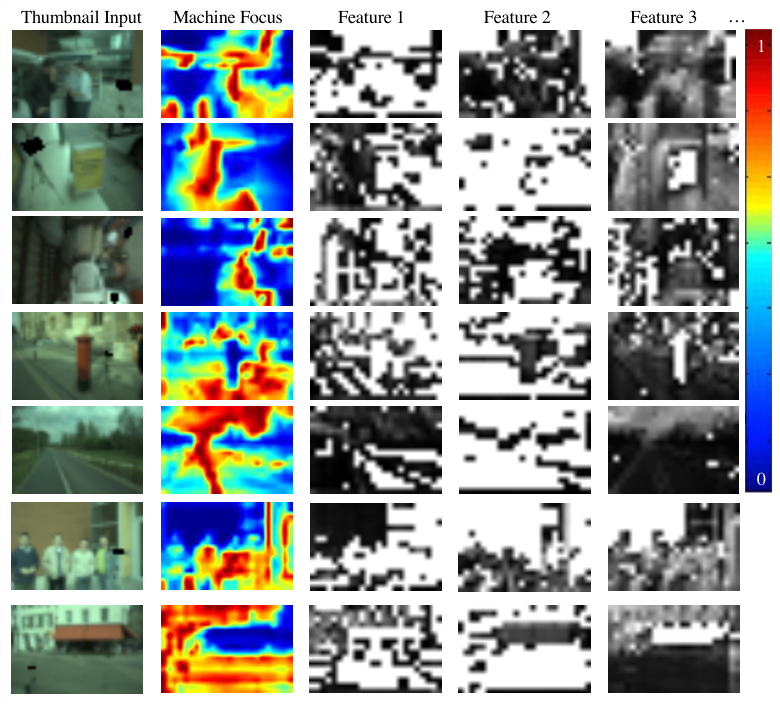
Since the final weighted per-channel global average pooling layer is essentially a fusion of all filtered image features, visualizing these filtered image features would be helpful to understand what has been learned. In Figure 3, given some inputs, we visualize the first 3 (of 14) channels of the learned intermediate features. We have observed both sparse features and smooth features, e.gFeature 3 looks relevant to colorfulness.
Since the final output is computed by per-channel averaging the last 3-channel network responses (after Conv2), most of the filtered pixel intensities should be close to the illuminant ground truth and the brighter pixels should contribute more to the final estimate. We convert the last 3-channel response image to a gray-scale image by taking a channel-wise average. In this gray-scale image, the brighter regions are more focused by our trained model for illuminant estimation. Some of these examples are shown in Figure 3. The trained model seems to focus on grayer surfaces for illuminant estimation. This pixel selectivity which CM offers is one of the fundamental differences compared with gray world [Buchsbaum(1980)] and gray edge [Van De Weijer et al.(2007a)Van De Weijer, Gevers, and Gijsenij].
5 Conclusion
We have presented Convolutional Mean (CM) – a simple and fast algorithm for illuminant estimation. Our proposed method accepts thumbnail input images for real-time processing (at least 30-60 frames per seconds with 5% computational budget) which is arguably 3-4500 faster than the other leading solutions. We have also shown that our proposed light-weight method offers accuracy comparable to the leading methods’ (which are relatively more parameter-demanding) across several measures. Future work would be a further reduction of model parameters, a full performance verification on embedded platforms, and a trail of other efficient statistics combined with machine-coded features.
Acknowledgements
The model training was carried out on the High Performance Computing Cluster supported by the Research and Specialist Computing Support service at the University of East Anglia. We thank NVIDIA for their generous donation of a GPU. We also thank the anonymous reviewers for their constructive feedback.
References
- [pyt()] Pytorch. URL https://pytorch.org/.
- [Afifi et al.(2019)Afifi, Punnappurath, Finlayson, and Brown] Mahmoud Afifi, Abhijith Punnappurath, Graham Finlayson, and Michael S Brown. As-projective-as-possible bias correction for illumination estimation algorithms. Journal of the Optical Society of America A, 36(1):71–78, 2019.
- [Ballerini et al.(2013)Ballerini, Fisher, Aldridge, and Rees] Lucia Ballerini, Robert B Fisher, Ben Aldridge, and Jonathan Rees. A color and texture based hierarchical k-nn approach to the classification of non-melanoma skin lesions. In Color Medical Image Analysis, pages 63–86. Springer, 2013.
- [Banic and Loncaric(2015)] Nikola Banic and Sven Loncaric. Color dog-guiding the global illumination estimation to better accuracy. In International Conference on Computer Vision Theory and Applications, pages 129–135, 2015.
- [Barnard et al.(2002)Barnard, Cardei, and Funt] Kobus Barnard, Vlad Cardei, and Brian Funt. A comparison of computational color constancy algorithms. i: Methodology and experiments with synthesized data. IEEE transactions on Image Processing, 11(9):972–984, 2002.
- [Barron(2015)] Jonathan T Barron. Convolutional color constancy. In IEEE International Conference on Computer Vision, pages 379–387, 2015.
- [Barron and Tsai(2017)] Jonathan T Barron and Yun-Ta Tsai. Fast fourier color constancy. In IEEE Conference on Computer Vision and Pattern Recognition, pages 886–894, 2017.
- [Barrow and Tenenbaum(1981)] Harry G Barrow and Jay M Tenenbaum. Computational vision. Proceedings of the IEEE, 69(5):572–595, 1981.
- [Bianco et al.(2010)Bianco, Ciocca, Cusano, and Schettini] Simone Bianco, Gianluigi Ciocca, Claudio Cusano, and Raimondo Schettini. Automatic color constancy algorithm selection and combination. Pattern recognition, 43(3):695–705, 2010.
- [Bianco et al.(2015)Bianco, Cusano, and Schettini] Simone Bianco, Claudio Cusano, and Raimondo Schettini. Color constancy using cnns. In IEEE Conference on Computer Vision and Pattern Recognition Workshops, pages 81–89, 2015.
- [Bianco et al.(2017)Bianco, Cusano, and Schettini] Simone Bianco, Claudio Cusano, and Raimondo Schettini. Single and multiple illuminant estimation using convolutional neural networks. IEEE Transactions on Image Processing, 26(9):4347–4362, 2017.
- [Brainard and Wandell(1986)] David H Brainard and Brian A Wandell. Analysis of the retinex theory of color vision. Journal of Optical Society of America A, 3(10):1651–1661, 1986.
- [Buchsbaum(1980)] Gershon Buchsbaum. A spatial processor model for object colour perception. Journal of the Franklin institute, 310(1):1–26, 1980.
- [Chakrabarti(2015)] Ayan Chakrabarti. Color constancy by learning to predict chromaticity from luminance. In Advances in Neural Information Processing Systems, pages 163–171, 2015.
- [Chakrabarti et al.(2012)Chakrabarti, Hirakawa, and Zickler] Ayan Chakrabarti, Keigo Hirakawa, and Todd Zickler. Color constancy with spatio-spectral statistics. IEEE Transactions on Pattern Analysis and Machine Intelligence, pages 1508–1517, 2012.
- [Cheng et al.(2014)Cheng, Prasad, and Brown] Dongliang Cheng, Dilip K Prasad, and Michael S Brown. Illuminant estimation for color constancy: why spatial-domain methods work and the role of the color distribution. JOSA A, 31(5):1049–1058, 2014.
- [Cheng et al.(2015)Cheng, Price, Cohen, and Brown] Dongliang Cheng, Brian Price, Scott Cohen, and Michael S Brown. Effective learning-based illuminant estimation using simple features. In IEEE Conference on Computer Vision and Pattern Recognition, pages 1000–1008, 2015.
- [Diederik P. Kingma(2014)] Jimmy Ba Diederik P. Kingma. Adam: A method for stochastic optimization. In International Conference on Learning Representations, 2014.
- [Dosovitskiy et al.(2015)Dosovitskiy, Fischer, Ilg, Hausser, Hazirbas, Golkov, Van Der Smagt, Cremers, and Brox] Alexey Dosovitskiy, Philipp Fischer, Eddy Ilg, Philip Hausser, Caner Hazirbas, Vladimir Golkov, Patrick Van Der Smagt, Daniel Cremers, and Thomas Brox. Flownet: Learning optical flow with convolutional networks. In IEEE international conference on computer vision, pages 2758–2766, 2015.
- [Finlayson et al.(2019)Finlayson, Gong, and Fisher] Graham Finlayson, Han Gong, and Robert B Fisher. Color homography: theory and applications. IEEE transactions on pattern analysis and machine intelligence, 41(1):20–33, 2019.
- [Finlayson(2013)] Graham D Finlayson. Corrected-moment illuminant estimation. In International Conference on Computer Vision, pages 1904–1911. IEEE, 2013.
- [Finlayson(2018)] Graham D Finlayson. Colour and illumination in computer vision. Interface focus, 8(4):20180008, 2018.
- [Finlayson and Trezzi(2004)] Graham D Finlayson and Elisabetta Trezzi. Shades of gray and colour constancy. In Color and Imaging Conference, volume 2004, pages 37–41. Society for Imaging Science and Technology, 2004.
- [Funt and Xiong(2004)] Brian Funt and Weihua Xiong. Estimating illumination chromaticity via support vector regression. In Color and Imaging Conference, volume 2004, pages 47–52. Society for Imaging Science and Technology, 2004.
- [Gao et al.(2014)Gao, Han, Yang, Li, and Li] Shaobing Gao, Wangwang Han, Kaifu Yang, Chaoyi Li, and Yongjie Li. Efficient color constancy with local surface reflectance statistics. In European Conference on Computer Vision, pages 158–173. Springer, 2014.
- [Gehler et al.(2008)Gehler, Rother, Blake, Minka, and Sharp] Peter Vincent Gehler, Carsten Rother, Andrew Blake, Tom Minka, and Toby Sharp. Bayesian color constancy revisited. In 2008 IEEE Conference on Computer Vision and Pattern Recognition, pages 1–8. IEEE, 2008.
- [Gijsenij and Gevers(2011a)] Arjan Gijsenij and Theo Gevers. Color constancy using natural image statistics and scene semantics. IEEE Transactions Pattern Analysis Machine Intelligence, 33(4):687–698, 2011a.
- [Gijsenij and Gevers(2011b)] Arjan Gijsenij and Theo Gevers. Color constancy using natural image statistics and scene semantics. IEEE Transactions on Pattern Analysis and Machine Intelligence, 33(4):687–698, 2011b.
- [Gijsenij et al.(2010)Gijsenij, Gevers, and Van De Weijer] Arjan Gijsenij, Theo Gevers, and Joost Van De Weijer. Generalized gamut mapping using image derivative structures for color constancy. International Journal of Computer Vision, 86(2-3):127–139, 2010.
- [Gijsenij et al.(2012)Gijsenij, Gevers, and Van De Weijer] Arjan Gijsenij, Theo Gevers, and Joost Van De Weijer. Improving color constancy by photometric edge weighting. IEEE Transactions on Pattern Analysis and Machine Intelligence, 34(5):918–929, 2012.
- [He et al.(2015)He, Zhang, Ren, and Sun] Kaiming He, Xiangyu Zhang, Shaoqing Ren, and Jian Sun. Delving deep into rectifiers: Surpassing human-level performance on imagenet classification. In IEEE international conference on computer vision, pages 1026–1034, 2015.
- [Hemrit et al.(2019)Hemrit, Matsushita, Uchida, Vazquez-Corral, Gong, Tsumura, and Finlayson] Ghalia Hemrit, Futa Matsushita, Mihiro Uchida, Javier Vazquez-Corral, Han Gong, Norimichi Tsumura, and Graham D Finlayson. Using the monge-kantorovitch transform in chromagenic color constancy for pathophysiology. In International Workshop on Computational Color Imaging, pages 121–133. Springer, 2019.
- [Hu et al.(2017)Hu, Wang, and Lin] Yuanming Hu, Baoyuan Wang, and Stephen Lin. Fc4: Fully convolutional color constancy with confidence-weighted pooling. In Conference on Computer Vision and Pattern Recognition, pages 4085–4094. IEEE, 2017.
- [Hubel et al.(2007)Hubel, Finlayson, and Hordley] Paul M Hubel, Graham D Finlayson, and Steven D Hordley. White point estimation using color by convolution, April 3 2007. US Patent 7,200,264.
- [Joze and Drew(2012)] Hamid Reza Vaezi Joze and Mark Drew. Exemplar-based colour constancy. In British Machine Vision Conference, pages 26.1–26.12. BMVA Press, 2012.
- [Shi and Funt()] L. Shi and B. Funt. Re-processed version of the gehler color constancy dataset of 568 images. URL http://www.cs.sfu.ca/~colour/data/shi_gehler/.
- [Shi et al.(2016)Shi, Loy, and Tang] Wu Shi, Chen Change Loy, and Xiaoou Tang. Deep specialized network for illuminant estimation. In European Conference on Computer Vision, pages 371–387. Springer, 2016.
- [Swain and Ballard(1991)] M.J. Swain and D.H.. Ballard. Color indexing. International Journal of Computer Vision, 7(11):11–32, 1991.
- [Van De Weijer et al.(2007a)Van De Weijer, Gevers, and Gijsenij] Joost Van De Weijer, Theo Gevers, and Arjan Gijsenij. Edge-based color constancy. IEEE Transactions on image processing, 16(9):2207–2214, 2007a.
- [Van De Weijer et al.(2007b)Van De Weijer, Schmid, and Verbeek] Joost Van De Weijer, Cordelia Schmid, and Jakob Verbeek. Using high-level visual information for color constancy. In International Conference on Computer Vision, pages 1–8. IEEE, 2007b.
- [Yang et al.(2015)Yang, Gao, and Li] Kai-Fu Yang, Shao-Bing Gao, and Yong-Jie Li. Efficient illuminant estimation for color constancy using grey pixels. In IEEE Conference on Computer Vision and Pattern Recognition, pages 2254–2263, 2015.