跳到论文正文
W Papers独立论文阅读器 arXiv:2001.04896 论文正文 计算阅读时间 · 0%
引用这篇论文根据当前论文元数据生成,正式投稿前建议核对。


License: arXiv.org perpetual non-exclusive license
arXiv:2001.04896v3 [math.ST] 26 Oct 2021

MINIMAX ADAPTIVE ESTIMATION IN MANIFOLD INFERENCE

Vincent Divol Affiliation: Center for Data Science and Courant Institute of Mathematical Science, New York University Email: firstname.lastname@nyu.edu Thanks:
Abstract

We focus on the problem of manifold estimation: given a set of observations sampled close to some unknown submanifold MM, one wants to recover information about the geometry of MM. Minimax estimators which have been proposed so far all depend crucially on the a priori knowledge of parameters quantifying the underlying distribution generating the sample (such as bounds on its density), whereas those quantities will be unknown in practice. Our contribution to the matter is twofold. First, we introduce a one-parameter family of manifold estimators (M^t)t≥0(\hat{M}_{t})_{t\geq 0} based on a localized version of convex hulls, and show that for some choice of tt, the corresponding estimator is minimax on the class of models of 𝒞2\mathcal{C}^{2} manifolds introduced in [GPPVW12]. Second, we propose a completely data-driven selection procedure for the parameter tt, leading to a minimax adaptive manifold estimator on this class of models. This selection procedure actually allows us to recover the Hausdorff distance between the set of observations and MM, and can therefore be used as a scale parameter in other settings, such as tangent space estimation.

1 Introduction

Manifold inference deals with the estimation of geometric quantities in a random setting. Given 𝒳n={X1,…,Xn}\mathcal{X}_{n}=\{X_{1},\dots,X_{n}\} a set of i.i.d. observations from some law μ\mu on ℝD\mathbb{R}^{D} supported on (or concentrated around) a dd-dimensional manifold MM, one wants to produce an estimator θ^\hat{\theta} that estimates accurately some quantity θ⁡(M)\theta(M) related to the geometry of MM such as its dimension dd [HA05, LJM09, KRW19], its homology groups [NSW08, BRS+12], its tangent spaces [AL19, CC16], or MM itself [GPPVW12, GPPIW12, MMS16, AL18, AL19, PS19]. Consider for instance the problem of estimating the manifold MM with respect to the Hausdorff distance dHd_{H}. The quality of an estimator M^\hat{M} with respect to some law μ\mu, called its μ\mu-risk, is given by the average Hausdorff distance dHd_{H} between the estimator and MM:

Rn​(M^,μ):=𝔼⁡[dH​(M^,M)],R_{n}(\hat{M},\mu)\vcentcolon=\mathbb{E}[d_{H}(\hat{M},M)], (1.1)

where M^=M^​(𝒳n)\hat{M}=\hat{M}(\mathcal{X}_{n}) and 𝒳n\mathcal{X}_{n} is a nn-sample of law μ\mu. In reality, the law μ\mu generating the dataset is unknown, and it is more interesting to control the μ\mu-risk uniformly over a set 𝒬\mathcal{Q} of laws μ\mu, that we call a statistical model. The uniform risk of the estimator M^\hat{M} on the class 𝒬\mathcal{Q} is given by,

Rn​(M^,𝒬):=sup{Rn​(M^,μ):μ∈𝒬}.R_{n}(\hat{M},\mathcal{Q})\vcentcolon=\sup\{R_{n}(\hat{M},\mu):\ \mu\in\mathcal{Q}\}. (1.2)

while we say that an estimator is minimax if it attains (up to a multiplicative constant as nn goes to ∞\infty) the minimax risk

ℛn​(𝒬):=inf{Rn​(M^,𝒬):M^​ is an estimator}.\mathcal{R}_{n}(\mathcal{Q})\vcentcolon=\inf\{R_{n}(\hat{M},\mathcal{Q}):\ \hat{M}\text{ is an estimator}\}. (1.3)
Figure 1: If the reach of the curve MM is large, then the curve cannot be too pinched (left) and cannot present a tight bottleneck structure (right).

In geometric inference, several statistical models were introduced, which take into account different noise models and regularities of the manifold MM. Let us mention the family of models 𝒬τmin,fmin,fmaxd\mathcal{Q}^{d}_{\tau_{\min},f_{\min},f_{\max}} introduced by Genovese et al. in [GPPVW12], consisting of the laws μ\mu supported on a dd-dimensional manifold MM satisfying some additional properties. First, we assume that μ\mu has a density ff on MM, lower bounded by some constant fmin>0f_{\min}>0 and upper bounded by another constant fmaxf_{\max}. This ensures that all the parts of the manifold MM are approximately evenly sampled: we then say that the law is "almost-uniform" on MM. The parameter τmin\tau_{\min} gives a lower bound on the reach τ⁡(M)\tau(M) of the manifold. The reach is a central notion in geometric inference, defined as the largest radius rr such that, if some point xx is at distance less than rr to MM, then there exists a unique projection πM​(x)\pi_{M}(x) of xx on MM. As such, it controls both a local regularity of MM (a bound on its curvature radius) and a global regularity (namely the presence of a "bottleneck structure"), see also Figure 1.

On the statistical model 𝒬τmin,fmin,fmaxd\mathcal{Q}^{d}_{\tau_{\min},f_{\min},f_{\max}}, the minimax rate of convergence satisfies

c0​(ln⁡nn)2/d≤ℛn​(𝒬τmin,fmin,fmaxd)≤c1​(ln⁡nn)2/d,c_{0}\left(\frac{\ln n}{n}\right)^{2/d}\leq\mathcal{R}_{n}(\mathcal{Q}^{d}_{\tau_{\min},f_{\min},f_{\max}})\leq c_{1}\left(\frac{\ln n}{n}\right)^{2/d}, (1.4)

for two positive constants c0c_{0}, c1c_{1} depending on τmin\tau_{\min}, fminf_{\min}, fmaxf_{\max} and dd. The lower bound in this inequality was shown by Kim and Zhou [KZ15], while the upper bound is obtained by exhibiting an estimator having a uniform risk of order (ln⁡n/n)2/d(\ln n/n)^{2/d}. Such an estimator (although not computable in practice) was first proposed by Genovese et al. in [GPPVW12], while another estimator attaining this same minimax rate (computable in practice), and based on the Tangential Delaunay Complex [BG14], was proposed by Aamari and Levrard [AL18]. Although being minimax and computable, the Tangential Delaunay Complex depends on the tuning of several parameters (for instance a radius quantifying the size of neighborhoods which are used to compute local PCAs), while those parameters have to be calibrated in a precise manner with respect to the quantities τmin\tau_{\min}, fminf_{\min} and fmaxf_{\max} defining the model for the Tangential Delauny Complex to be minimax. However, those quantities are a priori unknown. A first possibility is to estimate those quantities in turn: if procedures are known to estimate the reach (although themselves depending on the tuning of parameters [AKC+19, BHHS21]), estimating fminf_{\min} and fmaxf_{\max} appears to be delicate. The problem of the practical choice of the parameters defining the estimator is then raised. This question of the tuning of parameters defining an estimator is not restricted to the framework of manifold estimation, but is a classical problem in statistics.

Let us cite for instance the question of the choice of the bandwidth for kernel density estimation. Let X1,…,XnX_{1},\dots,X_{n} be a nn-sample of some law μ\mu having a density ff on ℝ\mathbb{R}, and suppose that we want to recover the value f⁡(x0)f(x_{0}) of the density at some fixed point x0∈ℝx_{0}\in\mathbb{R}. A standard method to achieve this goal is to consider the convolution of the empirical measure μn=1n​∑i=1nδXi\mu_{n}=\frac{1}{n}\sum_{i=1}^{n}\delta_{X_{i}} by some kernel KhK_{h}, where Kh=h−1K(⋅/h)K_{h}=h^{-1}K(\cdot/h) and KK satisfies ∫K=1\int K=1. We then obtain a function f^=Kh∗μn\hat{f}=K_{h}*\mu_{n}. Assume that the density ff is of regularity ss, that is f∈𝒞s​(ℝ)f\in\mathcal{C}^{s}(\mathbb{R}), the set of ⌊s⌋\lfloor s\rfloor-times differentiable functions, whose ⌊s⌋\lfloor s\rfloorth derivative is (s−⌊s⌋)(s-\lfloor s\rfloor)-Hölder continuous. Then, for a good choice of kernel KK, it is optimal to choose the bandwidth hopth_{\mathrm{opt}} of order c⋅n−1/(2s+1)c\cdot n^{-1/(2s+1)}, where cc depends on the 𝒞s\mathcal{C}^{s}-norm of ff [Tsy08, Chapter 1]. The associated risk is then of order n−s/(2s+1)n^{-s/(2s+1)}, which is the minimax rate of estimation on the class of densities of regularity ss. In practice, it is impossible to know exactly the value of ss, so that we must find another strategy to choose the bandwidth hh. Adaptive methods consist in choosing a bandwidth h^\hat{h} in a data-dependent way, such that the estimator f^h^\hat{f}_{\hat{h}} has a μ\mu-risk almost as good as the optimal estimator f^hopt\hat{f}_{h_{\mathrm{opt}}} under weak hypotheses on μ\mu. One of such methods, the PCO method (for Penalized Comparison to Overfitting) introduced by Lacour, Massart and Rivoirard [LMR17] consists in comparing each estimator f^h\hat{f}_{h} to some degenerate estimator f^hmin\hat{f}_{h_{\min}} for some very small bandwidth hminh_{\min}. The selected bandwidth h^\hat{h} is chosen among a family ℋ\mathcal{H} of bandwidths (all larger than hminh_{\min}), by minimizing a criterion depending on the distance ‖f^h−f^hmin‖L2​(ℝ)\|\hat{f}_{h}-\hat{f}_{h_{\min}}\|_{L_{2}(\mathbb{R})}, while penalizing small values of hh. Lacour, Massart and Rivoirard then show an oracle inequality for their estimator, that is an inequality of the form

𝔼​‖f^h^−f‖L2​(ℝ)2≤C​min⁡{𝔼​‖f^h−f‖L2​(ℝ)2:h∈ℋ}+C⁡(n,|ℋ|)\mathbb{E}\|\hat{f}_{\hat{h}}-f\|_{L_{2}(\mathbb{R})}^{2}\leq C\min\{\mathbb{E}\|\hat{f}_{h}-f\|^{2}_{L_{2}(\mathbb{R})}:\ h\in\mathcal{H}\}+C(n,|\mathcal{H}|) (1.5)

where C⁡(n,|ℋ|)C(n,|\mathcal{H}|) is a remainder term negligible in front of the optimal risk. Thus, we obtain that f^h^\hat{f}_{\hat{h}} has a risk almost as good as the best estimator f^hopt\hat{f}_{h_{\mathrm{opt}}}, while we never had to estimate the parameters defining the statistical model (that is the regularity ss of the density and the 𝒞s\mathcal{C}^{s}-norm of ff).

Figure 2: The tt-convex hull Conv(t,A)\Conv(t,A) (in green) of a curve AA (in black).

Our main goal is to adapt the PCO method to the manifold inference setting. A first step consists in creating a family of estimators (M^t)t≥0(\hat{M}_{t})_{t\geq 0} similar to kernel density estimators, but in the context of manifold estimation. This is made possible with tt-convex hulls. For t≥0t\geq 0, the tt-convex hull Conv(t,A)\Conv(t,A) of a set AA is an interpolation between the set AA (t=0t=0) and its convex hull Conv(A)\Conv(A) (t=∞t=\infty). It is defined as

Conv(t,A):=⋃σ⊆Ar⁡(σ)≤tConv(σ),\Conv(t,A)\vcentcolon=\bigcup_{\begin{subarray}{c}\sigma\subseteq A\\ r(\sigma)\leq t\end{subarray}}\Conv(\sigma), (1.6)

where r⁡(σ)r(\sigma) is the radius of the set σ\sigma, that is the radius of the smallest enclosing ball of σ\sigma. See Figure 2 for an example. We prove in Section 3 that for A⊆MA\subseteq M, the Hausdorff distance between Conv(t,A)\Conv(t,A) and MM can be efficiently controlled for values of tt a little larger than the approximation rate ε⁡(A):=sup{d⁡(x,A):x∈M}\varepsilon(A)\vcentcolon=\sup\{d(x,A):\ x\in M\} of AA. More precisely, for such values of tt, Lemma 3.3 states that dH​(Conv(t,A),M)≤t2/τ⁡(M)d_{H}(\Conv(t,A),M)\leq t^{2}/\tau(M). Using this control on the tt-convex hull enables us to show that the tt-convex hull of the sample 𝒳n\mathcal{X}_{n} is a minimax estimator on the model 𝒬τmin,fmin,fmaxd\mathcal{Q}^{d}_{\tau_{\min},f_{\min},f_{\max}} for a certain choice of tt.

Theorem 1.1.

Let αd\alpha_{d} be the volume of the dd-dimensional unit ball. For the choice of scale tn=74​(3​ln⁡n/(αd​fmin​n))1/dt_{n}=\frac{7}{4}(3\ln n/(\alpha_{d}f_{\min}n))^{1/d}, we have (for nn large enough)

Rn​(Conv(tn,𝒳n),𝒬τmin,fmin,fmaxd)≤c0τmin​(αd​fmin)2/d​(ln⁡nn)2/dR_{n}(\Conv(t_{n},\mathcal{X}_{n}),\mathcal{Q}^{d}_{\tau_{\min},f_{\min},f_{\max}})\leq\frac{c_{0}}{\tau_{\min}(\alpha_{d}f_{\min})^{2/d}}\left(\frac{\ln n}{n}\right)^{2/d} (1.7)

for some absolute constant c0c_{0}. In other words, Conv(tn,𝒳n)\Conv(t_{n},\mathcal{X}_{n}) is a minimax estimator of MM on 𝒬τmin,fmin,fmaxd\mathcal{Q}^{d}_{\tau_{\min},f_{\min},f_{\max}}.

To create an adaptive estimator, the next step is to build a selection procedure for the parameter tt. An analog of the degenerate estimator f^hmin\hat{f}_{h_{\min}} is given by the choice t=0t=0, with Conv(0,𝒳n)=𝒳n\Conv(0,\mathcal{X}_{n})=\mathcal{X}_{n}. The PCO method therefore suggests comparing the estimators Conv(t,𝒳n)\Conv(t,\mathcal{X}_{n}) with 𝒳n\mathcal{X}_{n}, that is to study the function t↦h⁡(t,𝒳n):=dH​(Conv(t,𝒳n),𝒳n)t\mapsto h(t,\mathcal{X}_{n})\vcentcolon=d_{H}(\Conv(t,\mathcal{X}_{n}),\mathcal{X}_{n}). The function h⁡(⋅,𝒳n)h(\cdot,\mathcal{X}_{n}) was actually already introduced under the name of "convexity defect function of the set 𝒳n\mathcal{X}_{n}" in a paper by Attali, Lieutier and Salinas [ALS13], where it was used to study the homotopy types of Rips complexes. The convexity defect function is nonnegative, nondecreasing, and satisfies 0≤h⁡(t,A)≤t0\leq h(t,A)\leq t for any set AA. For A=𝒳nA=\mathcal{X}_{n}, this function is piecewise constant, while it may only change values at t∈Rad(𝒳n):={r⁡(σ):σ⊆𝒳n}t\in\Rad(\mathcal{X}_{n})\vcentcolon=\{r(\sigma):\ \sigma\subseteq\mathcal{X}_{n}\}. We show that the convexity defect function h⁡(t,𝒳n)h(t,\mathcal{X}_{n}) of 𝒳n\mathcal{X}_{n} at scale tt exhibits different behaviors in two different regimes: for t≤ε⁡(𝒳n)t\leq\varepsilon(\mathcal{X}_{n}) it has a globally linear behavior (that is it stays close to its maximal value tt), whereas roughly after ε⁡(𝒳n)\varepsilon(\mathcal{X}_{n}), it is almost constant. The convexity defect function can be computed using only the dataset, so that we may in practice observe those two regimes. In practice, we fix a value 0<λ<10<\lambda<1, and let

tλ​(𝒳n):=inf{t∈Rad(𝒳n):h⁡(t,𝒳n)≤λ​t}.t_{\lambda}(\mathcal{X}_{n})\vcentcolon=\inf\{t\in\Rad(\mathcal{X}_{n}):\ h(t,\mathcal{X}_{n})\leq\lambda t\}. (1.8)

Our main result states that tλ​(𝒳n)t_{\lambda}(\mathcal{X}_{n}) is a little larger than ε⁡(𝒳n)\varepsilon(\mathcal{X}_{n}) with high probability, so that we may control the risk of M^=Conv(tλ​(𝒳n),𝒳n)\hat{M}=\Conv(t_{\lambda}(\mathcal{X}_{n}),\mathcal{X}_{n}), without having to know dd, fminf_{\min}, fmaxf_{\max} or the reach τ⁡(M)\tau(M), leading to an adaptive estimator in a sense made precise in Theorem 6.2. The estimator M^\hat{M} is to our knowledge the first minimax adaptive manifold estimator. Our procedure allows us to actually estimate (up to a multiplicative constant arbitrarily close to 11) the approximation rate ε⁡(𝒳n)\varepsilon(\mathcal{X}_{n}), while scale parameters in computational geometry typically have to be properly tuned with respect to this quantity. The parameter tλ​(𝒳n)t_{\lambda}(\mathcal{X}_{n}) can therefore be used as a hyperparameter in different settings. To illustrate this general idea, we show how to create a data-driven minimax estimator of the tangent spaces of a manifold (see Corollary 6.5).

Related work

"Localized" versions of convex hulls such as the tt-convex hulls have already been introduced in the support estimation literature. For instance, slightly modified versions of the t-convex hull have been used as estimators in [AB16] under the assumption that the support has a smooth boundary and in [RC07] under reach constraints on the support, with different rates obtained in those models. Selection procedures were not designed in those two papers, and whether our selection procedure leads to an adaptive estimator in those frameworks is an interesting question. The statistical models we study in this article were introduced in [GPPVW12] and [AL18], in which manifold estimators were also proposed. If the estimator in [GPPVW12] is of purely theoretical interest, the estimator proposed by Aamari and Levrard in [AL18], based on the Tangential Delaunay complex, is computable with 𝒪⁡(n​D​2𝒪⁡(d2))\mathcal{O}(nD2^{\mathcal{O}(d^{2})}) operations. Furthermore, it is a simplicial complex which is known to be ambient isotopic to the underlying manifold MM with high probability. It however requires the tuning of several hyperparameters in order to be minimax, which may make its use delicate in practice. In contrast, the tt-convex hull estimator with parameter tλ​(𝒳n)t_{\lambda}(\mathcal{X}_{n}) is completely data-driven, computable in polynomial time (see Section 7), while keeping the minimax property. However, unlike in the case of the Tangential Delaunay complex, we have no guarantees on the homotopy type of the corresponding estimator.

2 Background on submanifold with positive reach

Let us first introduce some notation. The Euclidean norm in ℝD\mathbb{R}^{D} is denoted by |⋅||\cdot| and ⟨⋅,⋅⟩\langle\cdot,\cdot\rangle stands for the dot product. If A⊆ℝDA\subseteq\mathbb{R}^{D} and x∈ℝDx\in\mathbb{R}^{D}, then d⁡(x,A):=inf{|x−y|:y∈A}d(x,A):=\inf\{|x-y|:y\in A\} is the distance to a set AA while diam(A):=sup{|x−y|:x,y∈A}\operatorname{diam}(A):=\sup\{|x-y|:x,y\in A\} is its diameter. Given r≥0r\geq 0, ℬ⁡(x,r)\mathcal{B}(x,r) is the open ball of radius rr centered at xx and we write ℬA​(x,r)\mathcal{B}_{A}(x,r) for ℬ⁡(x,r)∩A\mathcal{B}(x,r)\cap A. We let ℳd\mathcal{M}^{d} be the set of 𝒞2\mathcal{C}^{2} compact connected dd-dimensional submanifolds of ℝD\mathbb{R}^{D} without boundary. If M∈ℳdM\in\mathcal{M}^{d} and x∈Mx\in M, then Tx​MT_{x}M is the tangent space of MM at xx. It is identified with a dd-dimensional subspace of ℝD\mathbb{R}^{D}, and we write πx\pi_{x} for the orthogonal projection on Tx​MT_{x}M, while πx⟂=\pi_{x}^{\perp}= id −πx-\pi_{x} is the projection on the normal space Tx​M⟂T_{x}M^{\perp}. The asymmetric Hausdorff distance between sets A,B⊆ℝDA,B\subseteq\mathbb{R}^{D} is defined as dH​(A|B):=sup{d⁡(x,B):x∈A}d_{H}(A|B):=\sup\{d(x,B):x\in A\}, while the Hausdorff distance is defined as dH​(A,B)=max⁡{dH​(A|B),dH​(B|A)}d_{H}(A,B)=\max\left\{d_{H}(A|B),d_{H}(B|A)\right\}. For A⊆MA\subseteq M, we denote by ε⁡(A):=dH​(A,M)\varepsilon(A):=d_{H}(A,M) the approximation rate of AA.

The regularity of a submanifold M∈ℳdM\in\mathcal{M}^{d} is measured by its reach τ⁡(M)\tau(M). This is the largest number rr such that if d⁡(x,M)<rd(x,M)<r for x∈ℝDx\in\mathbb{R}^{D}, then there exists a unique point of MM, denoted by πM​(x)\pi_{M}(x), which is at distance d⁡(x,M)d(x,M) from xx. Thus, the projection πM\pi_{M} on the manifold MM is well-defined on the rr-tubular neigborhood Mr:={x∈M:d⁡(x,M)≤r}M^{r}:=\{x\in M:d(x,M)\leq r\} for r<τ⁡(M)r<\tau(M). The notion of reach was introduced for general sets by Federer in [Fed59], where it is also proven that 𝒞2\mathcal{C}^{2} compact submanifolds without boundary have positive reach (see [Fed59, p.432]). Different geometric quantities of interest can be bounded in term of the reach. For instance, the volume Vol⁡(M)\operatorname{Vol}(M) of MM satisfies

Vol⁡(M)≥ωd​τ​(M)d\operatorname{Vol}(M)\geq\omega_{d}\tau(M)^{d} (2.1)

where ωd\omega_{d} is the volume of a dd-dimensional sphere (with equality obtained only for a sphere of radius τ⁡(M)\tau(M)), see [Alm86]. The reach also controls how points on MM deviate from their projections on some tangent space.

Lemma 2.1 (Theorem 4.18 in [Fed59]).

For x,y∈Mx,y\in M, |πx⟂​(y−x)|≤|y−x|22​τ​(M)\left|\pi_{x}^{\perp}(y-x)\right|\leq\frac{|y-x|^{2}}{2\tau(M)}.

The following lemma asserts that the projection from a manifold to its tangent space is well-behaved.

Lemma 2.2.

Let x∈Mx\in M.

  1. 1.

    Let y∈ℝDy\in\mathbb{R}^{D} with d⁡(y,M)<τ⁡(M)d(y,M)<\tau(M). Then, πM​(y)=x\pi_{M}(y)=x if and only if y−x∈Tx​M⟂y-x\in T_{x}M^{\perp}.

  2. 2.

    Let y1,y2∈ℝDy_{1},y_{2}\in\mathbb{R}^{D} be two points at distance less than γ<τ⁡(M)\gamma<\tau(M) from MM. Then, |πM​(y1)−πM​(y2)|≤τ⁡(M)τ⁡(M)−γ​|y1−y2||\pi_{M}(y_{1})-\pi_{M}(y_{2})|\leq\frac{\tau(M)}{\tau(M)-\gamma}|y_{1}-y_{2}|.

  3. 3.

    For r<τ⁡(M)/3r<\tau(M)/3, the map π~x:y↦πx​(y−x)\tilde{\pi}_{x}:y\mapsto\pi_{x}(y-x) is a diffeomorphism from ℬM​(x,r)\mathcal{B}_{M}(x,r) to its image, and, if r≤τ⁡(M)/2r\leq\tau(M)/2, we have ℬTx​M​(0,7​r/8)⊆π~x​(ℬM​(x,r))\mathcal{B}_{T_{x}M}(0,7r/8)\subseteq\tilde{\pi}_{x}\left(\mathcal{B}_{M}(x,r)\right). In particular, if y∈ℬM​(x,7​τ​(M)/24)y\in\mathcal{B}_{M}(x,7\tau(M)/24), then

    78​|y−x|≤|πx​(y−x)|≤|y−x|.\frac{7}{8}|y-x|\leq\left|\pi_{x}(y-x)\right|\leq|y-x|. (2.2)
Proof.

∙\bullet For 1 and 2, see [Fed59, Theorem 4.8].

∙\bullet We first show that π~x\tilde{\pi}_{x} is injective on ℬM​(x,τ⁡(M)/3)\mathcal{B}_{M}(x,\tau(M)/3). Assume that π~x​(y)=π~x​(y′)\tilde{\pi}_{x}(y)=\tilde{\pi}_{x}\left(y^{\prime}\right) for some y≠y′∈My\neq y^{\prime}\in M. Consider without loss of generality that |x−y|≥|x−y′||x-y|\geq\left|x-y^{\prime}\right|. The goal is to show that |x−y|≥τ⁡(M)/3|x-y|\geq\tau(M)/3. If |x−y|>τ⁡(M)/2|x-y|>\tau(M)/2, the conclusion obviously holds, so we may assume that |x−y|≤τ⁡(M)/2|x-y|\leq\tau(M)/2. Define the angle between Tx​MT_{x}M and Ty​MT_{y}M as ‖πx−πy‖o​p\left\|\pi_{x}-\pi_{y}\right\|_{op} (where ∥⋅∥op \|\cdot\|_{\text{op }} denotes the operator norm). Lemma 3.43.4 in [BSW09] states that if |x−y|≤τ⁡(M)/2|x-y|\leq\tau(M)/2, then ∠⁡(Tx​M,Ty​M)≤2​|x−y|τ⁡(M)\angle\left(T_{x}M,T_{y}M\right)\leq 2\frac{|x-y|}{\tau(M)}. Also, by definition,

∠⁡(Tx​M,Ty​M)\displaystyle\angle\left(T_{x}M,T_{y}M\right) ≥|(πx−πy)​(y−y′)||y−y′|\displaystyle\geq\frac{\left|\left(\pi_{x}-\pi_{y}\right)\left(y-y^{\prime}\right)\right|}{\left|y-y^{\prime}\right|}
=|πy​(y−y′)||y−y′|≥|y−y′|−|πy⟂​(y−y′)||y−y′|\displaystyle=\frac{\left|\pi_{y}\left(y-y^{\prime}\right)\right|}{\left|y-y^{\prime}\right|}\geq\frac{\left|y-y^{\prime}\right|-\left|\pi_{y}^{\perp}\left(y-y^{\prime}\right)\right|}{\left|y-y^{\prime}\right|}
≥1−|y−y′|2​τ​(M)​ by Lemma 2.1\displaystyle\geq 1-\frac{\left|y-y^{\prime}\right|}{2\tau(M)}\text{ by Lemma \ref{lem2.1}}
≥1−|x−y|τ⁡(M)​ by the triangle inequality.\displaystyle\geq 1-\frac{|x-y|}{\tau(M)}\text{ by the triangle inequality. }

Therefore, we have 3​|x−y|/τ⁡(M)≥13|x-y|/\tau(M)\geq 1, i.e. |x−y|≥τ⁡(M)/3|x-y|\geq\tau(M)/3 and π~x\tilde{\pi}_{x} is injective on ℬM​(x,τ⁡(M)/3)\mathcal{B}_{M}(x,\tau(M)/3). To conclude that π~x\tilde{\pi}_{x} is a diffeomorphism, it suffices to show that its differential is always invertible. As π~x\tilde{\pi}_{x} is an affine application, the differential d​π~x​(y)d\tilde{\pi}_{x}(y) is equal to πx\pi_{x}. Therefore, the Jacobian of the function π~x:M→Tx​M\tilde{\pi}_{x}:M\rightarrow T_{x}M at yy is given by the determinant of the projection πx\pi_{x} restricted to Ty​MT_{y}M. In particular, it is larger than the smallest singular value of πx∘πy\pi_{x}\circ\pi_{y} to the power dd, which is larger than

(1−∠⁡(Tx​M,Ty​M))d≥(1−2​|x−y|τ⁡(M))d≥(13)d\left(1-\angle\left(T_{x}M,T_{y}M\right)\right)^{d}\geq\left(1-2\frac{|x-y|}{\tau(M)}\right)^{d}\geq\left(\frac{1}{3}\right)^{d}

thanks to [BSW09, Lemma 3.4] and using that |x−y|≤τ⁡(M)/3|x-y|\leq\tau(M)/3. In particular, the Jacobian is positive, and π~x\tilde{\pi}_{x} is a diffeormorphism from ℬM​(x,τ⁡(M)/3)\mathcal{B}_{M}(x,\tau(M)/3) to its image. The second statement is stated in [AL19, Lemma A.2].

The second inequality of the last statement follows from the projection being 1-Lipschitz continuous. For the first one, let y∈ℬM​(x,7​τ​(M)/24)y\in\mathcal{B}_{M}(x,7\tau(M)/24), and let u=u= πx​(y−x)\pi_{x}(y-x). The point uu is in ℬTx​M​(0,h)\mathcal{B}_{T_{x}M}(0,h) for h>|u|h>|u|. We have ℬTx​M​(0,h)⊆π~x​(ℬM​(x,8​h/7))⊆\mathcal{B}_{T_{x}M}(0,h)\subseteq\tilde{\pi}_{x}\left(\mathcal{B}_{M}(x,8h/7)\right)\subseteq π~x​(ℬM​(x,τ⁡(M)/3))\tilde{\pi}_{x}\left(\mathcal{B}_{M}(x,\tau(M)/3)\right). As π~x\tilde{\pi}_{x} is injective on ℬM​(x,τ⁡(M)/3)\mathcal{B}_{M}(x,\tau(M)/3), this means that we necessarily have y∈ℬM​(x,8​h/7)y\in\mathcal{B}_{M}(x,8h/7). Therefore, |x−y|<8​h/7|x-y|<8h/7, and the conclusion holds by letting hh goes to |u||u|. ∎

It will also be necessary to have precise bounds on the volume of balls on MM. As expected, the volume of a small ball is asymptotically equivalent to the volume of an Euclidean ball. Let αd\alpha_{d} be the volume of the dd-dimensional unit ball.

Lemma 2.3.

Let r≤τ⁡(M)/4r\leq\tau(M)/4 and x∈M.x\in M. Then,

(4748)d≤(1−r23​τ​(M)2)d≤Vol⁡(ℬM​(x,r))αd​rd≤(1+4​r23​τ​(M)2)d≤(1312)d.\left(\frac{47}{48}\right)^{d}\leq\left(1-\frac{r^{2}}{3\tau(M)^{2}}\right)^{d}\leq\frac{\operatorname{Vol}\left(\mathcal{B}_{M}(x,r)\right)}{\alpha_{d}r^{d}}\leq\left(1+\frac{4r^{2}}{3\tau(M)^{2}}\right)^{d}\leq\left(\frac{13}{12}\right)^{d}. (2.3)
Proof.

The proof of Proposition 8.7 in [AL18] implies that, if ℬ~M​(x,r)\tilde{\mathcal{B}}_{M}(x,r) is the geodesic ball centered at xx of radius rr, then

(1−r23​τ​(M)2)d≤Vol⁡(ℬ~M​(x,r))αd​rd≤(1+r2τ​(M)2)d.\left(1-\frac{r^{2}}{3\tau(M)^{2}}\right)^{d}\leq\frac{\operatorname{Vol}\left(\tilde{\mathcal{B}}_{M}(x,r)\right)}{\alpha_{d}r^{d}}\leq\left(1+\frac{r^{2}}{\tau(M)^{2}}\right)^{d}.

As ℬ~M​(x,r)⊆ℬM​(x,r)\tilde{\mathcal{B}}_{M}(x,r)\subseteq\mathcal{B}_{M}(x,r), we have in particular Vol⁡(ℬM​(x,r))αd​rd≥(1−r23​τ​(M)2)d\frac{\operatorname{Vol}\left(\mathcal{B}_{M}(x,r)\right)}{\alpha_{d}r^{d}}\geq\left(1-\frac{r^{2}}{3\tau(M)^{2}}\right)^{d}. Furthermore, by [ACLG19, Lemma 3.12] and [NSW08, Proposition 6.3], if |x−y|≤τ⁡(M)/4|x-y|\leq\tau(M)/4, then the geodesic distance between xx and yy is smaller than

|x−y|​(1+π250​τ​(M)2​|x−y|2)≤1.05​|x−y|.|x-y|\left(1+\frac{\pi^{2}}{50\tau(M)^{2}}|x-y|^{2}\right)\leq 1.05|x-y|.

This implies that ℬM​(x,r)⊆ℬ~M​(x,r⁡(1+π2​r250​τ​(M)2))\mathcal{B}_{M}(x,r)\subseteq\tilde{\mathcal{B}}_{M}\left(x,r\left(1+\frac{\pi^{2}r^{2}}{50\tau(M)^{2}}\right)\right). Therefore,

Vol⁡(ℬM​(x,r))αd​rd≤((1+π2​r250​τ​(M)2)​(1+(1.05​r)2τ​(M)2))d\displaystyle\frac{\operatorname{Vol}\left(\mathcal{B}_{M}(x,r)\right)}{\alpha_{d}r^{d}}\leq\left(\left(1+\frac{\pi^{2}r^{2}}{50\tau(M)^{2}}\right)\left(1+\frac{(1.05r)^{2}}{\tau(M)^{2}}\right)\right)^{d}
≤(1+(π250+(1.05)2+π2​(1.05)2​r250​τ​(M)2)​r2τ​(M)2)≤(1+4​r23​τ​(M)2)d,\displaystyle\leq\left(1+\left(\frac{\pi^{2}}{50}+(1.05)^{2}+\frac{\pi^{2}(1.05)^{2}r^{2}}{50\tau(M)^{2}}\right)\frac{r^{2}}{\tau(M)^{2}}\right)\leq\left(1+\frac{4r^{2}}{3\tau(M)^{2}}\right)^{d},

where we used at the last line that r≤τ⁡(M)/4r\leq\tau(M)/4. ∎

3 Approximation of manifolds with tt-convex hulls

Let A⊆MA\subseteq M be a finite set. We investigate in this section how the tt-convex hull of AA approximates MM for different values of tt, first in a deterministic setting, then in a random setting. The quantity of interest dH​(Conv⁡(t,A),M)d_{H}(\operatorname{Conv}(t,A),M) is by definition the maximum of the two quantities dH​(Conv⁡(t,A)|M)d_{H}(\operatorname{Conv}(t,A)|M) and dH​(M|Conv⁡(t,A))d_{H}(M|\operatorname{Conv}(t,A)). The first quantity dH​(Conv⁡(t,A)|M)d_{H}(\operatorname{Conv}(t,A)|M) is given by the maximum of the distances dH​(Conv⁡(σ)|M)d_{H}(\operatorname{Conv}(\sigma)|M) over the simplexes σ⊆A\sigma\subseteq A satisfying r⁡(σ)≤t.r(\sigma)\leq t. A naive attempt to bound this quantity leads to a control of order tt.

Lemma 3.1.

Let σ⊆ℝD\sigma\subseteq\mathbb{R}^{D} be a closed set. Then, dH​(Conv⁡(σ)|σ)≤r⁡(σ)d_{H}(\operatorname{Conv}(\sigma)|\sigma)\leq r(\sigma).

Proof.

Let y∈Conv⁡(σ)y\in\operatorname{Conv}(\sigma) and let zz be the center of the smallest enclosing ball of σ\sigma. The half-space {x∈ℝD:|x−z|2−r​(σ)2≤|x−y|2−d​(y,σ)2}\left\{x\in\mathbb{R}^{D}:|x-z|^{2}-r(\sigma)^{2}\leq|x-y|^{2}-d(y,\sigma)^{2}\right\} contains σ\sigma. It thus contains Conv⁡(σ)\operatorname{Conv}(\sigma), and in particular yy. Therefore, d​(y,σ)2≤r​(σ)2−|y−z|2≤r​(σ)2d(y,\sigma)^{2}\leq r(\sigma)^{2}-|y-z|^{2}\leq r(\sigma)^{2}, concluding the proof. ∎

As σ⊆M\sigma\subseteq M, we have in particular that dH​(Conv⁡(t,A)|M)≤td_{H}(\operatorname{Conv}(t,A)|M)\leq t. We can actually obtain a much better bound by exploiting that σ\sigma lies on MM, which looks locally like a flat space. Consider for instance the case where σ={x0,x1}\sigma=\left\{x_{0},x_{1}\right\} is made of two points. Then, the line (x0,x1)\left(x_{0},x_{1}\right) should be approximately parallel to the tangent space Tx0​MT_{x_{0}}M, with the distance from x1x_{1} to Tx0​MT_{x_{0}}M being of order |x0−x1|2\left|x_{0}-x_{1}\right|^{2}. As a consequence, the distance from any point of the segment [x0,x1]\left[x_{0},x_{1}\right] to MM is also of order |x0−x1|2\left|x_{0}-x_{1}\right|^{2}. More generally, we have the following result.

Lemma 3.2.

Let σ⊆M\sigma\subseteq M with r⁡(σ)<τ⁡(M)r(\sigma)<\tau(M) and let y∈Conv⁡(σ)y\in\operatorname{Conv}(\sigma). Then,

d⁡(y,M)≤τ⁡(M)​(1−1−r​(σ)2τ​(M)2)≤r​(σ)22​τ​(M)​(1+r​(σ)2τ​(M)2).d(y,M)\leq\tau(M)\left(1-\sqrt{1-\frac{r(\sigma)^{2}}{\tau(M)^{2}}}\right)\leq\frac{r(\sigma)^{2}}{2\tau(M)}\left(1+\frac{r(\sigma)^{2}}{\tau(M)^{2}}\right). (3.1)

In particular, for any t≥0t\geq 0 and A⊆MA\subseteq M,

dH​(Conv⁡(t,A)|M)≤t22​τ​(M)​[(1+t2τ​(M)2)∧2]≤t2τ⁡(M).d_{H}(\operatorname{Conv}(t,A)|M)\leq\frac{t^{2}}{2\tau(M)}\left[\left(1+\frac{t^{2}}{\tau(M)^{2}}\right)\wedge 2\right]\leq\frac{t^{2}}{\tau(M)}. (3.2)
Proof.

Lemma 12 in [ALS13] states that if σ⊆M\sigma\subseteq M satisfies r⁡(σ)<τ⁡(M)r(\sigma)<\tau(M) and y∈Conv⁡(σ)y\in\operatorname{Conv}(\sigma), then,

d⁡(y,M)≤τ⁡(M)​(1−1−r​(σ)2τ​(M)2).d(y,M)\leq\tau(M)\left(1-\sqrt{1-\frac{r(\sigma)^{2}}{\tau(M)^{2}}}\right).

As 1−u≥1−u/2−u2/2\sqrt{1-u}\geq 1-u/2-u^{2}/2 for u∈[0,1]u\in[0,1], one obtains the conclusion. ∎

The other asymmetric distance dH​(M|Conv⁡(t,A))d_{H}(M|\operatorname{Conv}(t,A)) is apparently more delicate to handle. It can actually be controlled efficiently if the parameter tt is large enough. Indeed, assume that tt is large enough so that every point xx of MM is the projection of some point yy of Conv⁡(t,A)\operatorname{Conv}(t,A). Then we have

d⁡(x,Conv⁡(t,A))≤|x−y|=|πM​(y)−y|=d⁡(y,M)≤dH​(Conv⁡(t,A)|M)≤t2τ⁡(M).\begin{split}d(x,\operatorname{Conv}(t,A))&\leq|x-y|=\left|\pi_{M}(y)-y\right|=d(y,M)\\ &\leq d_{H}(\operatorname{Conv}(t,A)|M)\leq\frac{t^{2}}{\tau(M)}.\end{split} (3.3)

This suggests defining the parameter

t∗​(A):=inf{t<τ⁡(M):πM​(Conv⁡(t,A))=M}.t^{*}(A):=\inf\left\{t<\tau(M):\pi_{M}(\operatorname{Conv}(t,A))=M\right\}. (3.4)

Lemma 3.2 and (3.3) imply directly the following lemma.

Figure 3: The tt-convex hull of the finite set AA (red crosses) is displayed (in green) for two values of tt. The black curve represents the (one dimensional) manifold MM. On the first display, the value of tt is smaller than t∗​(A)t^{*}(A), as there are regions of the manifold (circled in blue) which are not attained by the projection πM\pi_{M} restricted to the tt-convex hull. The value of tt is larger than t∗​(A)t^{*}(A) on the second display.
Lemma 3.3.

Let A⊆MA\subseteq M and t>t∗​(A)t>t^{*}(A). Then,

dH​(Conv⁡(t,A),M)≤t2τ⁡(M).d_{H}(\operatorname{Conv}(t,A),M)\leq\frac{t^{2}}{\tau(M)}. (3.5)

A crucial result in the analysis of the tt-convex hull estimator is given by the next proposition, that indicates that the quantity t∗​(A)t^{*}(A) is almost equal to the approximation rate ε⁡(A)\varepsilon(A).

Proposition 3.4.

Let A⊆MA\subseteq M be a finite set. Then, ε⁡(A)≤t∗​(A)​(1+t∗​(A)τ⁡(M)).\varepsilon(A)\leq t^{*}(A)\left(1+\frac{t^{*}(A)}{\tau(M)}\right). Furthermore, if ε⁡(A)<τ⁡(M)/8\varepsilon(A)<\tau(M)/8, then, t∗​(A)≤ε⁡(A)​(1+6​ε⁡(A)τ⁡(M))t^{*}(A)\leq\varepsilon(A)\left(1+6\frac{\varepsilon(A)}{\tau(M)}\right)

The proof of Proposition 3.4 relies on considering Delaunay triangulations. Given d+1d+1 points σ\sigma in ℝd\mathbb{R}^{d} that do not lie on a hyperplane, there exists a unique ball that contains the points on its boundary. It is called the circumball of σ\sigma, and its radius is called the circumradius circ⁡(σ)\mathrm{circ}(\sigma) of σ\sigma. Given a finite set A⊆ℝdA\subseteq\mathbb{R}^{d} that does not lie on a hyperplane, there exists a triangulation of AA, called the Delaunay triangulation, such that for each simplex σ\sigma in the triangulation, the circumball of σ\sigma contains no point of AA in its interior. Note that there may exist several Delaunay triangulations of a set AA, should the set AA not be in general position. With a slight abuse, we will still refer to "the" Delaunay triangulation of AA, by simply choosing a Delaunay triangulation among the possible ones should several exist. If the set AA lies on a lower dimensional subspace, we consider the Delaunay triangulation of AA in the affine vector space spanned by AA. Therefore, for every set AA, the Delaunay triangulation is well defined (for instance, the Delaunay triangulation of three points aligned in the plane is the 1-dimensional triangulation obtained by joining the middle point with the two others).

Proof.

Let x∈Mx\in M be such that d⁡(x,A)=ε⁡(A)d(x,A)=\varepsilon(A). By definition, there exists a simplex σ⊆A\sigma\subseteq A of radius smaller than t∗​(A)t^{*}(A) with x=πM​(y)x=\pi_{M}(y) for some point y∈Conv⁡(σ)y\in\operatorname{Conv}(\sigma). We have, using Lemma 3.1 and Lemma 3.2,

ε⁡(A)=d⁡(x,A)≤|x−y|+d⁡(y,A)≤t∗​(A)2τ⁡(M)+t∗​(A)\varepsilon(A)=d(x,A)\leq|x-y|+d(y,A)\leq\frac{t^{*}(A)^{2}}{\tau(M)}+t^{*}(A)

proving the first inequality.

To prove the other inequality, without loss of generality, we assume that 0∈M0\in M and we show that 0∈πM​(Conv⁡(t,A))0\in\pi_{M}(\operatorname{Conv}(t,A)) for t=ε⁡(A)​(1+6​ε​(A)/τ⁡(M)).t=\varepsilon(A)(1+6\varepsilon(A)/\tau(M)). Let A~=π0​(A∩ℬ⁡(0,R))\tilde{A}=\pi_{0}(A\cap\mathcal{B}(0,R)) for R=ε⁡(A)​(2+c0​ε​(A)/τ⁡(M))R=\varepsilon(A)\left(2+c_{0}\varepsilon(A)/\tau(M)\right) and c0=32/49c_{0}=32/49. Note that the condition ε⁡(A)≤τ⁡(M)/8\varepsilon(A)\leq\tau(M)/8 implies that R<7​τ​(M)/24R<7\tau(M)/24. We first state two lemmas.

Lemma 3.5.

Assume that ε⁡(A)≤7​τ​(M)/24\varepsilon(A)\leq 7\tau(M)/24. Let x~∈T0​M\tilde{x}\in T_{0}M with |x~|≤ε⁡(A).|\tilde{x}|\leq\varepsilon(A). Then d⁡(x~,A~)≤d(\tilde{x},\tilde{A})\leq ε⁡(A)\varepsilon(A).

Proof.

By continuity, it suffices to prove the claim for |x~|<ε⁡(A)|\tilde{x}|<\varepsilon(A). In this case, according to Lemma 2.2, if ε⁡(A)≤7​τ​(M)/24\varepsilon(A)\leq 7\tau(M)/24, then there exists x∈ℬM​(0,8​ε​(A)/7)x\in\mathcal{B}_{M}(0,8\varepsilon(A)/7) with π0​(x)=x~\pi_{0}(x)=\tilde{x}. Furthermore, by Lemma 2.1,

|x|≤|x~|+|x−x~|≤ε⁡(A)+|x|22​τ​(M)≤ε⁡(A)​(1+32​ε​(A)49​τ​(M)).|x|\leq|\tilde{x}|+|x-\tilde{x}|\leq\varepsilon(A)+\frac{|x|^{2}}{2\tau(M)}\leq\varepsilon(A)\left(1+\frac{32\varepsilon(A)}{49\tau(M)}\right).

We have d⁡(x,A)=|x−a|d(x,A)=|x-a| for some point a∈Aa\in A, and

|a|≤|x−a|+|x|≤ε⁡(A)​(2+c0​ε​(A)/τ⁡(M)).|a|\leq|x-a|+|x|\leq\varepsilon(A)\left(2+c_{0}\varepsilon(A)/\tau(M)\right).

As π0​(a)∈A~\pi_{0}(a)\in\tilde{A}, we have d⁡(x~,A~)≤|x~−π0​(a)|≤|x−a|=d⁡(x,A)≤ε⁡(A)d(\tilde{x},\tilde{A})\leq\left|\tilde{x}-\pi_{0}(a)\right|\leq|x-a|=d(x,A)\leq\varepsilon(A). ∎

Lemma 3.6.

Let V⊆ℝdV\subseteq\mathbb{R}^{d} be a finite set and t>0t>0. If dH​(ℬ⁡(0,t)|V)≤td_{H}(\mathcal{B}(0,t)|V)\leq t, then 0∈Conv⁡(V)0\in\operatorname{Conv}(V).

Proof.

We prove the contrapositive. If 0∉Conv⁡(V)0\notin\operatorname{Conv}(V), then there exists an open half-space which contains VV. Let xx be the unit vector orthogonal to this half-space. Then, d⁡(t​x,V)>td(tx,V)>t. ∎

Apply Lemma 3.6 to V=A~V=\tilde{A} and t=ε⁡(A)t=\varepsilon(A). For x~∈ℬT0​M​(0,ε⁡(A))\tilde{x}\in\mathcal{B}_{T_{0}M}(0,\varepsilon(A)), we have d⁡(x~,A~)≤ε⁡(A)d(\tilde{x},\tilde{A})\leq\varepsilon(A) according to Lemma 3.5. Therefore, we have 0∈Conv⁡(A~)0\in\operatorname{Conv}(\tilde{A}). Consider the Delaunay triangulation of A~\tilde{A}. The point 0 belongs to the convex hull of some simplex σ~\tilde{\sigma} of the triangulation, with circumradius circ⁡(σ~)\mathrm{circ}(\tilde{\sigma}) and center of the circumball q~\tilde{q}. The simplex σ~\tilde{\sigma} corresponds to some simplex σ\sigma in AA, and the point 0 is equal to π0​(y)\pi_{0}(y) for some point y∈Conv⁡(σ)y\in\operatorname{Conv}(\sigma). By Lemma 2.2, we actually have πM​(y)=0\pi_{M}(y)=0, and to conclude, it suffices to show that r⁡(σ)≤ε⁡(A)​(1+6​ε⁡(A)τ⁡(M))r(\sigma)\leq\varepsilon(A)\left(1+6\frac{\varepsilon(A)}{\tau(M)}\right). To do so, we use the next lemma (recall that σ⊆ℬM​(0,R)\sigma\subseteq\mathcal{B}_{M}(0,R) with OPENR<7​τ​(M)/24)\left.R<7\tau(M)/24\right).

Lemma 3.7.

Let σ⊆ℬM​(0,7​τ​(M)/24)\sigma\subseteq\mathcal{B}_{M}(0,7\tau(M)/24) and σ~=π~0​(σ)\tilde{\sigma}=\tilde{\pi}_{0}(\sigma). Assume that 0∈Conv⁡(σ~)0\in\operatorname{Conv}(\tilde{\sigma}). Then,

r⁡(σ~)≤r⁡(σ)≤r⁡(σ~)​(1+6​r⁡(σ~)τ⁡(M)).r(\tilde{\sigma})\leq r(\sigma)\leq r(\tilde{\sigma})\left(1+6\frac{r(\tilde{\sigma})}{\tau(M)}\right). (3.6)
Proof.

As the projection is 1-Lipschitz, it is clear that r⁡(σ~)≤r⁡(σ)r(\tilde{\sigma})\leq r(\sigma). Let us prove the other inequality. Let σ={y0,…,yk},σ~={y~0,…,y~k}\sigma=\left\{y_{0},\ldots,y_{k}\right\},\tilde{\sigma}=\left\{\tilde{y}_{0},\ldots,\tilde{y}_{k}\right\} and fix 0≤i≤k.0\leq i\leq k. As yi∈ℬM​(0,7​τ​(M)/24)y_{i}\in\mathcal{B}_{M}(0,7\tau(M)/24), we have by (2.2)

|yi|≤87​|y~i|≤167​r​(σ~).\left|y_{i}\right|\leq\frac{8}{7}\left|\tilde{y}_{i}\right|\leq\frac{16}{7}r(\tilde{\sigma}). (3.7)

where we used that |y~i|≤2​r​(σ~)\left|\tilde{y}_{i}\right|\leq 2r(\tilde{\sigma}) as 0∈Conv⁡(σ~)0\in\operatorname{Conv}(\tilde{\sigma}). Let z~\tilde{z} be the center of the minimum enclosing ball of σ~\tilde{\sigma}. Write z~=∑j=0kλj​y~j\tilde{z}=\sum_{j=0}^{k}\lambda_{j}\tilde{y}_{j} as a convex combination of the y~j\tilde{y}_{j}s and let z=∑j=0kλj​yj∈z=\sum_{j=0}^{k}\lambda_{j}y_{j}\in Conv⁡(σ)\operatorname{Conv}(\sigma). Then, we have

|z−yi|\displaystyle\left|z-y_{i}\right| ≤|z−z~|+|z~−y~i|+|y~i−yi|\displaystyle\leq|z-\tilde{z}|+\left|\tilde{z}-\tilde{y}_{i}\right|+\left|\tilde{y}_{i}-y_{i}\right|
≤∑j=0kλj​|yj−y~j|+r⁡(σ~)+|yi|22​τ​(M)​ using Lemma 2.1\displaystyle\leq\sum_{j=0}^{k}\lambda_{j}\left|y_{j}-\tilde{y}_{j}\right|+r(\tilde{\sigma})+\frac{\left|y_{i}\right|^{2}}{2\tau(M)}\text{ using Lemma \ref{lem2.1}}
≤∑j=0kλj​|yj|22​τ​(M)+r⁡(σ~)+12849​r​(σ~)2τ⁡(M)​ using Lemma 2.1 and (3.7)\displaystyle\leq\sum_{j=0}^{k}\lambda_{j}\frac{\left|y_{j}\right|^{2}}{2\tau(M)}+r(\tilde{\sigma})+\frac{128}{49}\frac{r(\tilde{\sigma})^{2}}{\tau(M)}\text{ using Lemma \ref{lem2.1} and \eqref{eq3.7}}
≤r⁡(σ~)+25649​r​(σ~)2τ⁡(M)≤r⁡(σ~)+6​r​(σ~)2τ⁡(M)​ using (3.7).\displaystyle\leq r(\tilde{\sigma})+\frac{256}{49}\frac{r(\tilde{\sigma})^{2}}{\tau(M)}\leq r(\tilde{\sigma})+6\frac{r(\tilde{\sigma})^{2}}{\tau(M)}\text{ using \eqref{eq3.7}. }

We obtain the conclusion as σ\sigma is included in the ball of radius maxi⁡|z−yi|\max_{i}\left|z-y_{i}\right| and center zz. ∎

Using the previous lemma, we are left with showing that r⁡(σ~)≤ε⁡(A)r(\tilde{\sigma})\leq\varepsilon(A). We will actually show the stronger inequality circ⁡(σ~)≤ε⁡(A)\operatorname{circ}(\tilde{\sigma})\leq\varepsilon(A) (the radius of a set is always smaller than its circumradius). As 0 is in the circumball (that is centered at q~\tilde{q}), the ball centered at q~\tilde{q} of radius |q~||\tilde{q}| does not intersect A~\tilde{A}. This enforces |q~|≤ε⁡(A)|\tilde{q}|\leq\varepsilon(A): otherwise, there would exist a ball not intersecting A~\tilde{A}, of radius ε⁡(A)\varepsilon(A), and whose center is at distance less than ε⁡(A)\varepsilon(A) from 0, a contradiction with Lemma 3.5 (see Figure 4). As |q~|≤ε⁡(A)|\tilde{q}|\leq\varepsilon(A), we obtain, once again according to Lemma 3.5, that circ⁡(σ~)=d⁡(q~,A~)≤ε⁡(A)\operatorname{circ}(\tilde{\sigma})=d(\tilde{q},\tilde{A})\leq\varepsilon(A) concluding the proof. ∎

Figure 4: If |q~|>ε⁡(A)|\tilde{q}|>\varepsilon(A), then the ball ℬT0​M​(q~,|q~|)\mathcal{B}_{T_{0}M}(\tilde{q},|\tilde{q}|) contains a ball of radius ε⁡(A)\varepsilon(A) centered at a point (here denoted by w~\tilde{w}) at distance less than ε⁡(A)\varepsilon(A) from 0.
Remark 3.8.

In the case where the dimension dd is known, one can consider a variant of the tt-convex hull, Convd⁡(t,A)\operatorname{Conv}_{d}(t,A), where one restricts the union to be over simplices of dimension less than dd. The set Convd⁡(t,A)\operatorname{Conv}_{d}(t,A) is simpler to compute as it contains less simplices (see Section 7). Furthermore, if td∗​(A):=inf{t:πM​(Convd⁡(t,A))=M}t_{d}^{*}(A):=\inf\left\{t:\pi_{M}(\operatorname{Conv}_{d}(t,A))=M\right\}, then both Lemma 3.3 and Proposition 3.4 hold with td∗​(A)t_{d}^{*}(A) and Convd⁡(t,A)\operatorname{Conv}_{d}(t,A) instead of t∗​(A)t^{*}(A) and Conv⁡(t,A)\operatorname{Conv}(t,A). Indeed, only simplices of dimension less than dd (corresponding to simplices of a Delaunay triangulation on a tangent space) were considered in the previous proof.

We have now shown that the quality of the tt-convex hull on AA can be controlled for t≥ε⁡(A)​(1+6​ε​(A)/τ⁡(M))t\geq\varepsilon(A)(1+6\varepsilon(A)/\tau(M)) (that is slightly larger than the approximation rate OPENε⁡(A))\varepsilon(A)). In a random setting, the approximation rate is known to be of order (ln⁡n/n)1/d(\ln n/n)^{1/d}: this is enough to show that the tt-convex hull is a minimax estimator. Recall the definition of the statistical model 𝒬τmin,fmin,fmaxd\mathcal{Q}_{\tau_{\min},f_{\min},f_{\max}}^{d} from the introduction: it consists of laws μ\mu supported on some manifold M∈ℳdM\in\mathcal{M}^{d} with τ⁡(M)≥τmin\tau(M)\geq\tau_{\min}, having a density ff lower bounded by fminf_{\min} and upper bounded by fmaxf_{\max}. The minimax result will actually hold on the larger model 𝒬τmin,fmind:=⋃fmax𝒬τmin,fmin,fmaxd\mathcal{Q}_{\tau_{\min},f_{\min}}^{d}:=\bigcup_{f_{\max}}\mathcal{Q}_{\tau_{\min},f_{\min},f_{\max}}^{d} (that is without imposing any upper bound on ff).

Let μ∈𝒬τmin,fmind\mu\in\mathcal{Q}_{\tau_{\min},f_{\min}}^{d} and let 𝒳n\mathcal{X}_{n} be a nn-sample from law μ\mu. We consider the estimator Conv⁡(t,𝒳n)\operatorname{Conv}(t,\mathcal{X}_{n}). Note first that Conv⁡(t,𝒳n)\operatorname{Conv}(t,\mathcal{X}_{n}) is indeed an estimator, that is the application

(x1,…,xn)∈(ℝD)n↦Conv⁡(t,{x1,…,xn})\left(x_{1},\ldots,x_{n}\right)\in\left(\mathbb{R}^{D}\right)^{n}\mapsto\operatorname{Conv}(t,\left\{x_{1},\ldots,x_{n}\right\})

is measurable (with respect to the Borel σ\sigma-field associated with the metric dHd_{H} on the set 𝒦⁡(ℝD)\mathcal{K}\left(\mathbb{R}^{D}\right) of all nonempty compact subsets of ℝD\mathbb{R}^{D}). Indeed, for EE a measurable subset of 𝒦⁡(ℝD)\mathcal{K}\left(\mathbb{R}^{D}\right) and A,B∈𝒦⁡(ℝD)A,B\in\mathcal{K}\left(\mathbb{R}^{D}\right), introduce the notation GE​(A,B)=AG_{E}(A,B)=A if A∈EA\in E and BB otherwise. This function is measurable, and Conv⁡(t,{x1,…,xn})\operatorname{Conv}(t,\left\{x_{1},\ldots,x_{n}\right\}) can be written as

⋃I⊆{1,…,n}GE​(Conv⁡({xi}i∈I),{xi}i∈I)\bigcup_{I\subseteq\{1,\ldots,n\}}G_{E}\left(\operatorname{Conv}(\left\{x_{i}\right\}_{i\in I}\right),\left\{x_{i}\right\}_{i\in I})

where EE is the subset of 𝒦⁡(ℝD)\mathcal{K}\left(\mathbb{R}^{D}\right) given by {K∈𝒦⁡(ℝD):r⁡(K)≤t}\left\{K\in\mathcal{K}\left(\mathbb{R}^{D}\right):r(K)\leq t\right\}, which is closed [ALS13, Lemma 16]. As the functions ∪\cup and Conv are measurable, the measurability follows [Aam17, Proposition III.7].

For a fixed t>0t>0, we obtain the following control of 𝔼⁡[dH​(Conv⁡(t,𝒳n),M)].\mathbb{E}\left[d_{H}(\operatorname{Conv}(t,\mathcal{X}_{n}),M)\right].

𝔼⁡[dH​(Conv⁡(t,𝒳n),M)]\displaystyle\mathbb{E}\left[d_{H}(\operatorname{Conv}(t,\mathcal{X}_{n}),M)\right] =𝔼[dH(Conv(t,𝒳n),M)𝟏{t≥t∗(𝒳n)}]\displaystyle=\mathbb{E}\left[d_{H}(\operatorname{Conv}(t,\mathcal{X}_{n}),M)\mathbf{1}\left\{t\geq t^{*}(\mathcal{X}_{n})\right\}\right]
+𝔼[dH(Conv(t,𝒳n),M)𝟏{t<t∗(𝒳n)}]\displaystyle+\mathbb{E}\left[d_{H}(\operatorname{Conv}(t,\mathcal{X}_{n}),M)\mathbf{1}\left\{t<t^{*}(\mathcal{X}_{n})\right\}\right]
≤t2τ⁡(M)+diam⁡(M)​ℙ​(t∗​(𝒳n)>t)\displaystyle\leq\frac{t^{2}}{\tau(M)}+\operatorname{diam}(M)\mathbb{P}\left(t^{*}(\mathcal{X}_{n})>t\right)

By Proposition 3.4, if ε⁡(𝒳n)<τ⁡(M)/8\varepsilon(\mathcal{X}_{n})<\tau(M)/8, then

t∗​(𝒳n)≤ε⁡(𝒳n)​(1+6​ε⁡(𝒳n)τ⁡(M))≤74​ε​(𝒳n).t^{*}(\mathcal{X}_{n})\leq\varepsilon(\mathcal{X}_{n})\left(1+6\frac{\varepsilon(\mathcal{X}_{n})}{\tau(M)}\right)\leq\frac{7}{4}\varepsilon(\mathcal{X}_{n}).

Therefore, if tt is small enough,

ℙ⁡(t∗​(𝒳n)>t)\displaystyle\mathbb{P}\left(t^{*}(\mathcal{X}_{n})>t\right) ≤ℙ⁡(ε⁡(𝒳n)>τ⁡(M)/8)+ℙ⁡(ε⁡(𝒳n)>4​t/7)\displaystyle\leq\mathbb{P}\left(\varepsilon(\mathcal{X}_{n})>\tau(M)/8\right)+\mathbb{P}\left(\varepsilon(\mathcal{X}_{n})>4t/7\right)
≤2​ℙ​(ε⁡(𝒳n)>4​t/7).\displaystyle\leq 2\mathbb{P}\left(\varepsilon(\mathcal{X}_{n})>4t/7\right).

We obtain

𝔼⁡[dH​(Conv⁡(t,𝒳n),M)]≤t2τ⁡(M)+2​diam⁡(M)​ℙ​(ε⁡(𝒳n)>4​t/7)\mathbb{E}\left[d_{H}(\operatorname{Conv}(t,\mathcal{X}_{n}),M)\right]\leq\frac{t^{2}}{\tau(M)}+2\operatorname{diam}(M)\mathbb{P}\left(\varepsilon(\mathcal{X}_{n})>4t/7\right) (3.8)

Hence, to control the risk, it suffices to bound the tail of ε⁡(𝒳n)\varepsilon(\mathcal{X}_{n}).

Proposition 3.9.

Let μ∈𝒬τmin,fmind\mu\in\mathcal{Q}_{\tau_{\min},f_{\min}}^{d} and let 𝒳n={X1,…,Xn}\mathcal{X}_{n}=\left\{X_{1},\ldots,X_{n}\right\} be a nn-sample of law μ.\mu. If r≤τmin/4r\leq\tau_{\min}/4, then, for any η∈(0,1)\eta\in(0,1)

ℙ⁡(ε⁡(𝒳n)>r)≤cd,ηfmin​rd​exp⁡(−n​αd​fmin​(1−r23​τmin2)d​η​rd),\mathbb{P}\left(\varepsilon(\mathcal{X}_{n})>r\right)\leq\frac{c_{d,\eta}}{f_{\min}r^{d}}\exp\left(-n\alpha_{d}f_{\min}\left(1-\frac{r^{2}}{3\tau_{\min}^{2}}\right)^{d}\eta r^{d}\right), (3.9)

where cd,ηc_{d,\eta} depends on dd and η\eta. Furthermore, for any a>0a>0, for nn large enough (with respect to dd, fmin,τminf_{\min},\tau_{\min} and aa), with probability 1−c​(ln⁡n)d−1​n1−a1-c(\ln n)^{d-1}n^{1-a} (where c depends also on those parameters), we have

ε⁡(𝒳n)≤(a​ln⁡nαd​fmin​n)1/d.\varepsilon(\mathcal{X}_{n})\leq\left(\frac{a\ln n}{\alpha_{d}f_{\min}n}\right)^{1/d}. (3.10)
Proof.

A measure ν\nu is said to be (a,b)(a,b)-standard at scale r0r_{0} if ν⁡(ℬ⁡(x,r))≥a​rb\nu(\mathcal{B}(x,r))\geq ar^{b} for all r≤r0r\leq r_{0} and xx in the support of ν\nu. Let μ∈𝒬τmin,fmind\mu\in\mathcal{Q}_{\tau_{\min},f_{\min}}^{d} with support MM. Lemma 2.3 indicates that the measure μ\mu is (a,b)(a,b)-standard at scale r0r_{0} for any r0≤τ⁡(M)/4r_{0}\leq\tau(M)/4, with a=fmin​αd​(1−r023​τ​(M)2)da=f_{\min}\alpha_{d}\left(1-\frac{r_{0}^{2}}{3\tau(M)^{2}}\right)^{d} and b=db=d. It is stated in the proof [Aam17, Proposition III.14] that for such a measure, and for any δ≤2​r0\delta\leq 2r_{0} with 0<r−δ≤r00<r-\delta\leq r_{0}, we have

ℙ⁡(ε⁡(𝒳n)>r)≤2ba​δb​exp⁡(−n​a​(r−δ)b).\mathbb{P}\left(\varepsilon(\mathcal{X}_{n})>r\right)\leq\frac{2^{b}}{a\delta^{b}}\exp\left(-na(r-\delta)^{b}\right).

Letting r=r0r=r_{0} and δ=(1−η1/d)​r\delta=\left(1-\eta^{1/d}\right)r for some η∈(0,1)\eta\in(0,1), we obtain that

ℙ⁡(ε⁡(𝒳n)>r)≤(2/(1−η1/d))dfmin​αd​(1−r23​τ​(M)2)d​rd​exp⁡(−n​fmin​αd​(1−r23​τ​(M)2)d​η​rd)\displaystyle\mathbb{P}\left(\varepsilon(\mathcal{X}_{n})>r\right)\leq\frac{\left(2/\left(1-\eta^{1/d}\right)\right)^{d}}{f_{\min}\alpha_{d}\left(1-\frac{r^{2}}{3\tau(M)^{2}}\right)^{d}r^{d}}\exp\left(-nf_{\min}\alpha_{d}\left(1-\frac{r^{2}}{3\tau(M)^{2}}\right)^{d}\eta r^{d}\right) (3.11)
≤c0dfmin​αd​rd​exp⁡(−n​fmin​αd​(1−r23​τ​(M)2)d​η​rd)\displaystyle\leq\frac{c_{0}^{d}}{f_{\min}\alpha_{d}r^{d}}\exp\left(-nf_{\min}\alpha_{d}\left(1-\frac{r^{2}}{3\tau(M)^{2}}\right)^{d}\eta r^{d}\right)

for c0=96/(47​(1−η1/d))c_{0}=96/\left(47\left(1-\eta^{1/d}\right)\right), where we used at the last line that r≤τ⁡(M)/4r\leq\tau(M)/4.

To prove the second statement, we let r=(a​ln⁡nαd​fmin​n)1/dr=\left(\frac{a\ln n}{\alpha_{d}f_{\min}n}\right)^{1/d}. Then, we have n​αd​fmin​rd=a​ln⁡nn\alpha_{d}f_{\min}r^{d}=a\ln n. Letting η=1−1/ln⁡n\eta=1-1/\ln n, we obtain that

n​fmin​αd​(1−r23​τ​(M)2)d​η​rd\displaystyle nf_{\min}\alpha_{d}\left(1-\frac{r^{2}}{3\tau(M)^{2}}\right)^{d}\eta r^{d} =(a​ln⁡n)​(1−1ln⁡n)​(1−c​(ln⁡nn)2/d)\displaystyle=(a\ln n)\left(1-\frac{1}{\ln n}\right)\left(1-c\left(\frac{\ln n}{n}\right)^{2/d}\right)
≥(a​ln⁡n)−Ca.\displaystyle\geq(a\ln n)-C_{a}.

In particular, we obtain that the upper bound in (3.11) is of order (ln⁡n)d−1​n1−a(\ln n)^{d-1}n^{1-a}. ∎

Choose tt such that 4​t/7=(3​ln⁡nαd​fmin⁡n​n)1/d4t/7=\left(\frac{3\ln n}{\alpha_{d}f_{\min n}n}\right)^{1/d}. Then, according to Proposition 3.9, we have ℙ⁡(ε⁡(𝒳n)>32​t/7)≤c​(ln⁡n)d−1​n−2.\mathbb{P}\left(\varepsilon(\mathcal{X}_{n})>32t/7\right)\leq c(\ln n)^{d-1}n^{-2}. As diam⁡(M)\operatorname{diam}(M) is also bounded by a constant depending on τmin,fmin\tau_{\min},f_{\min} and dd (see [Aam17, Lemma III.24]), we obtain Theorem 1.1 from (3.8) (without even the need of assuming that the density ff is upper bounded).

4 Selection procedure for the tt-convex hulls

Assuming that we have observed a nn-sample 𝒳n\mathcal{X}_{n} having a distribution μ∈𝒫τmin,fmind\mu\in\mathcal{P}_{\tau_{\min},f_{\min}}^{d}, we were able in the previous section to build a minimax estimator of the underlying manifold MM. The tuning of this estimator requires the knowledge of dd and fminf_{\min}: if the dimension dd can be efficiently estimated, this is not the case for fminf_{\min}, which will likely not be accessible in practice. An idea to overcome this issue is to design a selection procedure for the family of estimators (Conv⁡(t,𝒳n))t≥0\left(\operatorname{Conv}(t,\mathcal{X}_{n})\right)_{t\geq 0}. As the loss of the estimator Conv⁡(t,𝒳n)\operatorname{Conv}(t,\mathcal{X}_{n}) is controlled efficiently for t≥t∗​(𝒳n)t\geq t^{*}(\mathcal{X}_{n}) a good idea is to select a scale tt larger than t∗​(𝒳n)t^{*}(\mathcal{X}_{n}). We however do not have access to this quantity based on the observations 𝒳n\mathcal{X}_{n}, as the manifold MM is unknown. To select a scale close to t∗​(𝒳n)t^{*}(\mathcal{X}_{n}), we monitor how the estimators Conv⁡(t,𝒳n)\operatorname{Conv}(t,\mathcal{X}_{n}) deviate from 𝒳n\mathcal{X}_{n} as tt increases. Namely, we use the convexity defect function introduced in [ALS13].

Definition 4.1.

Let A⊆ℝDA\subseteq\mathbb{R}^{D} and t>0t>0. The convexity defect function at scale t of AA is defined a​sas

h⁡(t,A):=dH​(Conv⁡(t,A),A).h(t,A):=d_{H}(\operatorname{Conv}(t,A),A). (4.1)

As its name indicates, the convexity defect function measures the (lack of) convexity of a set AA at a given scale tt. The next proposition states preliminary results on the convexity defect function.

Proposition 4.2.

Let A⊆ℝDA\subseteq\mathbb{R}^{D} be a closed set and t≥0t\geq 0.

  1. 1.

    We have 0≤h⁡(t,A)≤t0\leq h(t,A)\leq t.

  2. 2.

    The set AA is convex if and only if h⁡(⋅,A)≡0h(\cdot,A)\equiv 0.

  3. 3.

    If M∈ℳdM\in\mathcal{M}^{d}, then h⁡(t,M)≤t22​τ​(M)​(1+t2τ​(M)2)h(t,M)\leq\frac{t^{2}}{2\tau(M)}\left(1+\frac{t^{2}}{\tau(M)^{2}}\right).

Proof.

Point 1 follows from Lemma 3.1. Point 2 is clear and Point 3 is a consequence of Lemma 3.2. ∎

Refer to caption      Refer to caption

Refer to caption      Refer to caption

Figure 5: Two subsets of the torus having the same approximation rate, but whose convexity defect functions exhibit different behaviors on [0,t∗​(A)]\left[0,t^{*}(A)\right].

As expected, the convexity defect of a convex set is null, whereas for small values of tt, the convexity defect of a manifold h⁡(t,M)h(t,M) is very small (compared to the maximum value possible, which is tt): when looked at locally, MM is "almost flat" (and thus "almost locally convex"). As already noted in the introduction, if AA is a finite set, then the convexity defect function is a piecewise constant function, whose value may only change at tt if t∈Rad⁡(A):={r⁡(σ):σ⊆A}t\in\operatorname{Rad}(A):=\{r(\sigma):\sigma\subseteq A\}.

For a set A⊆MA\subseteq M, we recover the subquadratic behavior of the convexity defect function for values of tt above the threshold value t∗​(A)t^{*}(A). Namely, we have the following proposition.

Proposition 4.3.

Let A⊆MA\subseteq M. For t∗​(A)<t<τ⁡(M)t^{*}(A)<t<\tau(M),

h⁡(t,A)≤t22​τ​(M)​(1+t2τ​(M)2)+t∗​(A)​(1+t∗​(A)τ⁡(M)).h(t,A)\leq\frac{t^{2}}{2\tau(M)}\left(1+\frac{t^{2}}{\tau(M)^{2}}\right)+t^{*}(A)\left(1+\frac{t^{*}(A)}{\tau(M)}\right). (4.2)
Proof.

By using that h⁡(t,A)≤th(t,A)\leq t and Lemma 3.3, for any t∗​(A)<s<tt^{*}(A)<s<t,

h⁡(t,A)\displaystyle h(t,A) =dH​(Conv⁡(t,A),A)\displaystyle=d_{H}(\operatorname{Conv}(t,A),A)
≤dH​(Conv⁡(t,A),M)+dH​(M,Conv⁡(s,A))+dH​(Conv⁡(s,A),A)\displaystyle\leq d_{H}(\operatorname{Conv}(t,A),M)+d_{H}(M,\operatorname{Conv}(s,A))+d_{H}(\operatorname{Conv}(s,A),A)
≤t22​τ​(M)​(1+t2τ​(M)2)+s22​τ​(M)​(1+s2τ​(M)2)+s\displaystyle\leq\frac{t^{2}}{2\tau(M)}\left(1+\frac{t^{2}}{\tau(M)^{2}}\right)+\frac{s^{2}}{2\tau(M)}\left(1+\frac{s^{2}}{\tau(M)^{2}}\right)+s

The conclusion is obtained by letting ss go to t∗​(A)t^{*}(A). ∎

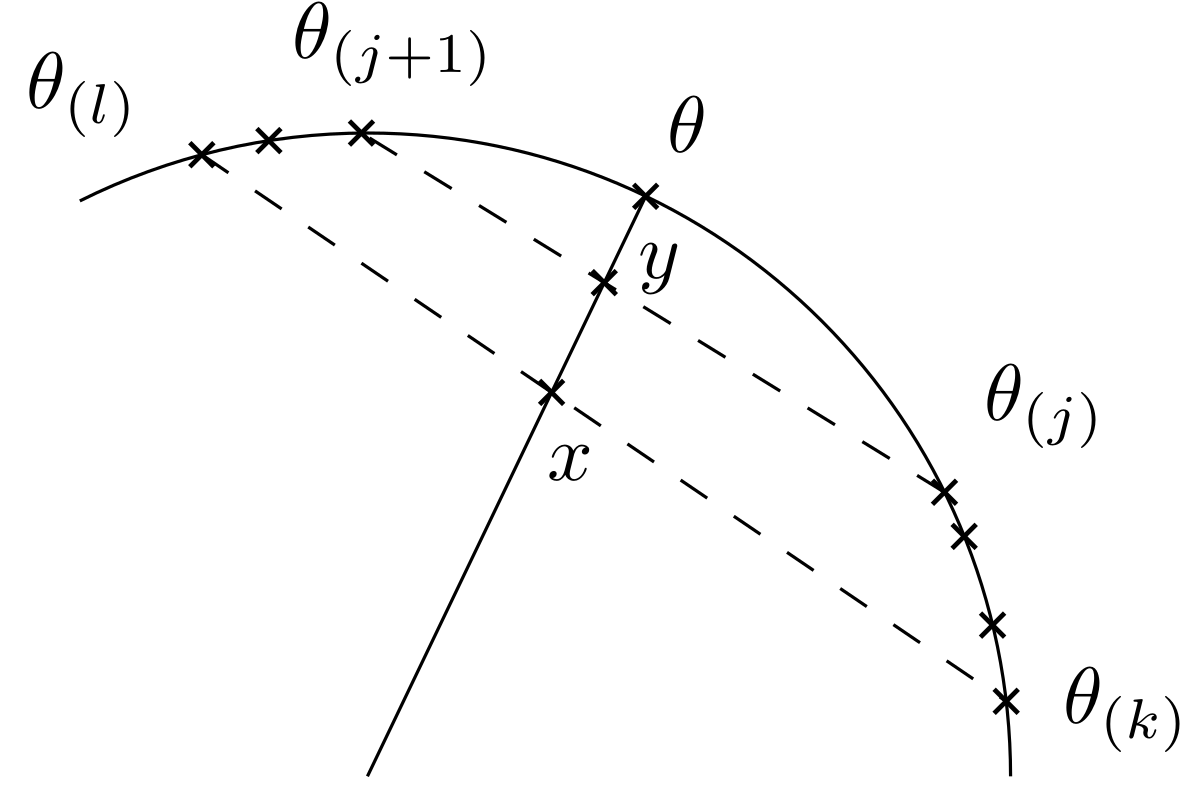
For 0<t<t∗​(A)0<t<t^{*}(A), the convexity defect function may exhibit very different behaviors, as shown in Figure 5. However, when the set A=𝒳nA=\mathcal{X}_{n} is a random nn-sample, it appears that the graph of the convexity defect function stays close to the diagonal {x=y}\{x=y\} for small values of tt. This is explained by the fact that for two points X1,X2X_{1},X_{2} in the sample at very small distance 2​t2t from one another, it is very unlikely that there is a third point at distance of order tt from X1X_{1} and X2X_{2}, so that dH​(Conv⁡({X1,X2})|𝒳n)=dH​(Conv⁡({X1,X2})|{X1,X2})=td_{H}(\operatorname{Conv}(\left\{X_{1},X_{2}\right\})|\mathcal{X}_{n})=d_{H}(\operatorname{Conv}(\left\{X_{1},X_{2}\right\})|\left\{X_{1},X_{2}\right\})=t.

This suggests the following strategy to select a value of tt larger than t∗​(𝒳n)t^{*}(\mathcal{X}_{n}) using the convexity defect function:

Definition 4.4.

Let A⊆MA\subseteq M be a finite set and 0<λ≤10<\lambda\leq 1. We define

tλ​(A):=inf{t∈Rad⁡(A):h⁡(t,A)≤λ​t}.t_{\lambda}(A):=\inf\{t\in\operatorname{Rad}(A):h(t,A)\leq\lambda t\}. (4.3)

Restricting to values t∈Rad⁡(A)t\in\operatorname{Rad}(A) is necessary, for otherwise we would always have tλ​(A)=t_{\lambda}(A)= 0 (as h⁡(t,A)=0h(t,A)=0 for tt small enough). Proposition 4.3 implies that tλ​(A)t_{\lambda}(A) cannot be too large. More precisely, we have the following lemma.

Lemma 4.5.

Let A⊆MA\subseteq M with t∗​(A)≤λ2​τ​(M)/4t^{*}(A)\leq\lambda^{2}\tau(M)/4. Let r0=t∗​(A)λ​(1+8λ2​t∗​(A)τ⁡(M))r_{0}=\frac{t^{*}(A)}{\lambda}\left(1+\frac{8}{\lambda^{2}}\frac{t^{*}(A)}{\tau(M)}\right) and r1=r_{1}= λ​τ​(M)/2.\lambda\tau(M)/2. If t∈Rad⁡(A)∩[r0,r1]t\in\operatorname{Rad}(A)\cap\left[r_{0},r_{1}\right], then tλ​(A)≤tt_{\lambda}(A)\leq t.

Proof.

By Proposition 4.3, we have, for t∗​(A)<t≤λ​τ​(M)/2t^{*}(A)<t\leq\lambda\tau(M)/2,

h⁡(t,A)\displaystyle h(t,A) ≤t22​τ​(M)​(1+t2τ​(M)2)+t∗​(A)​(1+t∗​(A)τ⁡(M))\displaystyle\leq\frac{t^{2}}{2\tau(M)}\left(1+\frac{t^{2}}{\tau(M)^{2}}\right)+t^{*}(A)\left(1+\frac{t^{*}(A)}{\tau(M)}\right)
≤t22​τ​(M)​(1+λ2/4)+t∗​(A)​(1+t∗​(A)τ⁡(M))−λ​t+λ​t=:P⁡(t)+λ​t.\displaystyle\leq\frac{t^{2}}{2\tau(M)}\left(1+\lambda^{2}/4\right)+t^{*}(A)\left(1+\frac{t^{*}(A)}{\tau(M)}\right)-\lambda t+\lambda t=:P(t)+\lambda t.

Let u=2​t∗​(A)​(1+t∗​(A)τ⁡(M))​(1+λ2/4)/(λ2​τ​(M))u=2t^{*}(A)\left(1+\frac{t^{*}(A)}{\tau(M)}\right)\left(1+\lambda^{2}/4\right)/\left(\lambda^{2}\tau(M)\right). The condition t∗​(A)≤λ2​τ​(M)/4t^{*}(A)\leq\lambda^{2}\tau(M)/4 ensures that u≤1u\leq 1. The quantity P⁡(t)P(t) is nonpositive if tt is between t0t_{0} and t1t_{1}, where

t0=τ⁡(M)​λ1+λ2/4​(1−1−u) and t1=τ⁡(M)​λ1+λ2/4​(1+1−u).t_{0}=\frac{\tau(M)\lambda}{1+\lambda^{2}/4}(1-\sqrt{1-u})\quad\text{ and }\quad t_{1}=\frac{\tau(M)\lambda}{1+\lambda^{2}/4}(1+\sqrt{1-u}).

We have t1≥r1t_{1}\geq r_{1} and, using the inequality 1−u≥1−u2−u22\sqrt{1-u}\geq 1-\frac{u}{2}-\frac{u^{2}}{2} for 0≤u≤10\leq u\leq 1, we obtain that t0≤r0t_{0}\leq r_{0}. Therefore, any t∈[r0,r1]t\in\left[r_{0},r_{1}\right] satisfies h⁡(t,A)≤λ​th(t,A)\leq\lambda t (note that r0>t∗​(A)r_{0}>t^{*}(A)). In particular, if tt is also in Rad⁡(A)\operatorname{Rad}(A), we have tλ​(A)≤tt_{\lambda}(A)\leq t. ∎

Our main theorem states that, with high probability, the parameter tλ​(𝒳n)t_{\lambda}(\mathcal{X}_{n}) is larger than t∗​(𝒳n)t^{*}(\mathcal{X}_{n})

Theorem 4.6.
  1. 1.

    Let μ∈𝒬τmin,fmin,fmaxd\mu\in\mathcal{Q}_{\tau_{\min},f_{\min},f_{\max}}^{d}. Let 0<b≤20<b\leq 2 and let 𝒳n\mathcal{X}_{n} be a n-sample of law μ\mu. Let a=(d−1)∨2a=(d-1)\vee 2 if b=2b=2, and a=d−1a=d-1 otherwise. For nn large enough, and with probability larger than 1−c​(ln⁡n)a​n−b1-c(\ln n)^{a}n^{-b}, we have for 0<λ<(1+b)−1/d0<\lambda<(1+b)^{-1/d},

    t∗​(𝒳n)≤tλ​(𝒳n)≤t∗​(𝒳n)λ​(1+C​((ln⁡n)2n)1/d)t^{*}(\mathcal{X}_{n})\leq t_{\lambda}(\mathcal{X}_{n})\leq\frac{t^{*}(\mathcal{X}_{n})}{\lambda}\left(1+C\left(\frac{(\ln n)^{2}}{n}\right)^{1/d}\right) (4.4)

    where the constant cc depends on bb, and μ\mu, and CC depends on fminf_{\min}, fmaxf_{\max}, dd, τmin\tau_{\min} and λ\lambda.

  2. 2.

    Furthermore, if μ\mu is the uniform distribution on the circle of radius τmin\tau_{\min}, then, for λ>(1+b)−1\lambda>(1+b)^{-1}, we have

    ℙ⁡(t∗​(𝒳n)>tλ​(𝒳n))≥c​n−b\mathbb{P}\left(t^{*}(\mathcal{X}_{n})>t_{\lambda}(\mathcal{X}_{n})\right)\geq cn^{-b} (4.5)

    for some constant c depending on τmin\tau_{\min} and bb.

Inequality (4.5) implies that the probability 1−c​(ln⁡n)a​n−b1-c(\ln n)^{a}n^{-b} appearing in the theorem is close to being tight.

Proof of the upper bound in (4.4)

Let μ∈𝒬τmin,fmin,fmaxd\mu\in\mathcal{Q}_{\tau_{\min},f_{\min},f_{\max}}^{d} be a probability distribution with support MM and density ff. We assume without loss of generality that fminf_{\min} is the essential infimum of ff. Recall the notation r1=λ​τ​(M)/2r_{1}=\lambda\tau(M)/2 and r0=t∗​(𝒳n)λ​(1+8λ2​t∗​(𝒳n)τ⁡(M))r_{0}=\frac{t^{*}(\mathcal{X}_{n})}{\lambda}\left(1+\frac{8}{\lambda^{2}}\frac{t^{*}(\mathcal{X}_{n})}{\tau(M)}\right) from Lemma 4.5. The proof of the upper bound is based on the following lemma.

Lemma 4.7.

There exists a positive constant β>0\beta>0 (depending on fmin,fmax,df_{\min},f_{\max},d and 𝑂𝑃𝐸𝑁τmin)\left.\tau_{\min}\right) such that the following holds. Let α>0\alpha>0 and let I=[a,b]I=[a,b] be an interval of length at least ℓ=α​(ln⁡nn)2/d\ell=\alpha\left(\frac{\ln n}{n}\right)^{2/d} with b≤β​α​(ln⁡nn)1/db\leq\beta\alpha\left(\frac{\ln n}{n}\right)^{1/d} and a≥ℓ/2a\geq\ell/2. Then, the probability that Rad⁡(𝒳n)\operatorname{Rad}(\mathcal{X}_{n}) does not intersect II is smaller than n−1/2n^{-1/2}.

Before proving the lemma, let us use it to obtain the upper bound in (4.4). By Proposition 3.9 and Proposition 3.4, we have t∗​(𝒳n)≤(4​ln⁡nαd​fmin⁡n)1/dt^{*}(\mathcal{X}_{n})\leq\left(\frac{4\ln n}{\alpha_{d}f_{\min n}}\right)^{1/d} everywhere but on a set of probability smaller than n−2n^{-2}. We will assume that this condition is satisfied. In particular, the condition t∗​(𝒳n)≤λ2​τ​(M)/4t^{*}(\mathcal{X}_{n})\leq\lambda^{2}\tau(M)/4 of Lemma 4.5 is satisfied. Let u=δ​((ln⁡n)2n)1/du=\delta\left(\frac{(\ln n)^{2}}{n}\right)^{1/d} (for some constant δ\delta to fix) and let

R0:=r0​(1+u)≤t∗​(𝒳n)λ​(1+2​δ​((ln⁡n)2n)1/d)≤2λ​(4​ln⁡nαd​fmin​n)1/d≤r1.R_{0}:=r_{0}(1+u)\leq\frac{t^{*}(\mathcal{X}_{n})}{\lambda}\left(1+2\delta\left(\frac{(\ln n)^{2}}{n}\right)^{1/d}\right)\leq\frac{2}{\lambda}\left(\frac{4\ln n}{\alpha_{d}f_{\min}n}\right)^{1/d}\leq r_{1}.
Lemma 4.8.

Let A⊆MA\subseteq M be a finite set of cardinality nn. Then,

ε(A)≥cdτ(M)n−1/d.\varepsilon(A)\geq c_{d}\tau(M)n^{-1/d}.
Proof.

If ε⁡(A)≥τ⁡(M)/4\varepsilon(A)\geq\tau(M)/4, the conclusion holds. Otherwise, as M⊆⋃x∈AℬM​(x,ε⁡(A))M\subseteq\bigcup_{x\in A}\mathcal{B}_{M}(x,\varepsilon(A)), one has Vol⁡(M)≤n​cd​ε​(A)d\operatorname{Vol}(M)\leq nc_{d}\varepsilon(A)^{d} (using Lemma 2.3). We conclude with inequality (2.1). ∎

According to Lemma 4.8 and Proposition 3.4, the interval [r0,R0]\left[r_{0},R_{0}\right] is of length r0​u≥r_{0}u\geq C1​δ​(ln⁡nn)2/d=:ℓC_{1}\delta\left(\frac{\ln n}{n}\right)^{2/d}=:\ell for some constant C1C_{1}. Choose δ\delta large enough so that 2λ​(4αd​fmin)1/d≤β​C1​δ\frac{2}{\lambda}\left(\frac{4}{\alpha_{d}f_{\min}}\right)^{1/d}\leq\beta C_{1}\delta. Then, as r0≥ℓ/2r_{0}\geq\ell/2 (once again by Lemma 4.8), one can apply Lemma 4.7: the interval [r0,R0]\left[r_{0},R_{0}\right] intersects Rad⁡(𝒳n)\operatorname{Rad}(\mathcal{X}_{n}) with probability 1−n−21-n^{-2}. Lemma 4.5 then yields the conclusion.

Proof of Lemma 4.7.

Let Ik=[k​ℓ/2,(k+1)​ℓ/2]I_{k}=[k\ell/2,(k+1)\ell/2] for kk an integer. Assume that we show that Rad⁡(𝒳n)\operatorname{Rad}(\mathcal{X}_{n}) intersects every interval IkI_{k} for k=1,…,Kk=1,\ldots,K, where KK is chosen so that b≤b\leq β​α​(ln⁡nn)1/d≤(K+1)​ℓ/2\beta\alpha\left(\frac{\ln n}{n}\right)^{1/d}\leq(K+1)\ell/2, say K+1=⌈2​β​α​(ln⁡nn)1/d/ℓ⌉=⌈2​β​(n/ln⁡n)1/d⌉K+1=\left\lceil 2\beta\alpha\left(\frac{\ln n}{n}\right)^{1/d}/\ell\right\rceil=\left\lceil 2\beta(n/\ln n)^{1/d}\right\rceil. As the interval II is of length at least ℓ\ell, and as ℓ/2≤a\ell/2\leq a, the interval II contains one of the interval IkI_{k} for some 1≤k≤K1\leq k\leq K. In particular, the interval II also intersects 𝒳n.\mathcal{X}_{n}. Therefore, it suffices to bound the probability that Rad⁡(𝒳n)\operatorname{Rad}(\mathcal{X}_{n}) does not intersect IkI_{k}. If we show that this probability is of order at most n−3n^{-3}, we may then conclude by a union bound: the probability that Rad⁡(𝒳n)\operatorname{Rad}(\mathcal{X}_{n}) intersects all the IkI_{k} is larger than 1−2​K​n−3≥1−4​β​n1/d−3/(ln⁡n)1/d≥1−n−2.1-2Kn^{-3}\geq 1-4\beta n^{1/d-3}/(\ln n)^{1/d}\geq 1-n^{-2}.

To bound the probability that Rad⁡(𝒳n)\operatorname{Rad}(\mathcal{X}_{n}) does not intersect IkI_{k}, we split the set 𝒳n\mathcal{X}_{n} into two groups: the set 𝒳n0={X1,…,XL}\mathcal{X}_{n}^{0}=\left\{X_{1},\ldots,X_{L}\right\} (for some integer LL to fix), and the set 𝒳n1={XL+1,…,Xn}\mathcal{X}_{n}^{1}=\left\{X_{L+1},\ldots,X_{n}\right\}. If some distance |Xi−Xj|\left|X_{i}-X_{j}\right| is between k​ℓk\ell and (k+1)​ℓ(k+1)\ell, then Rad⁡(𝒳n)\operatorname{Rad}(\mathcal{X}_{n}) intersects IkI_{k}. We will show that it is very likely that |Xi−Xj|∈[k​ℓ,(k+1)​ℓ]\left|X_{i}-X_{j}\right|\in[k\ell,(k+1)\ell] for some i≤Li\leq L and j>Lj>L. To do so, we consider the ball BiB_{i} centered at the point XiX_{i}, of radius (k+1)​ℓ(k+1)\ell. Let YY be a point sampled according to μ\mu, conditioned on being in BiB_{i}. Then, according to Lemma 2.3, we have

ℙ⁡(|Y−Xi|∈[k​ℓ,(k+1)​ℓ]|Xi)=μ⁡(ℬ⁡(Xi,(k+1)​ℓ)\ℬ⁡(Xi,k​ℓ))μ⁡(ℬ⁡(Xi,(k+1)​ℓ))\displaystyle\mathbb{P}\left(\left|Y-X_{i}\right|\in[k\ell,(k+1)\ell]|X_{i}\right)=\frac{\mu\left(\mathcal{B}\left(X_{i},(k+1)\ell\right)\backslash\mathcal{B}\left(X_{i},k\ell\right)\right)}{\mu\left(\mathcal{B}\left(X_{i},(k+1)\ell\right)\right)}
≥cd​fminfmax​(k+1)d​((k+1)d​(1−(k+1)2​ℓ23​τ​(M)2)d−kd​(1+4​k2​ℓ23​τ​(M)2)d)\displaystyle\geq\frac{c_{d}f_{\min}}{f_{\max}(k+1)^{d}}\left((k+1)^{d}\left(1-\frac{(k+1)^{2}\ell^{2}}{3\tau(M)^{2}}\right)^{d}-k^{d}\left(1+\frac{4k^{2}\ell^{2}}{3\tau(M)^{2}}\right)^{d}\right)
≥cd​fminfmax​(k+1)d​(d​kd−1​(1−(k+1)2​ℓ23​τ​(M)2)d−CLOSE\displaystyle\geq\frac{c_{d}f_{\min}}{f_{\max}(k+1)^{d}}\Bigg(dk^{d-1}\left(1-\frac{(k+1)^{2}\ell^{2}}{3\tau(M)^{2}}\right)^{d}-
OPENkd​((1+4​k2​ℓ23​τ​(M)2)d−(1−(k+1)2​ℓ23​τ​(M)2)d))\displaystyle k^{d}\left(\left(1+\frac{4k^{2}\ell^{2}}{3\tau(M)^{2}}\right)^{d}-\left(1-\frac{(k+1)^{2}\ell^{2}}{3\tau(M)^{2}}\right)^{d}\right)\Bigg)
≥cd​fminfmax​(k+1)d​(d​kd−1/2−C4​kd​k2​ℓ2τ​(M)2)≥C5k\displaystyle\geq\frac{c_{d}f_{\min}}{f_{\max}(k+1)^{d}}\left(dk^{d-1}/2-C_{4}k^{d}\frac{k^{2}\ell^{2}}{\tau(M)^{2}}\right)\geq\frac{C_{5}}{k}

where we used the inequality C4​k2​ℓ2τ​(M)2≤d​k−1/4C_{4}\frac{k^{2}\ell^{2}}{\tau(M)^{2}}\leq dk^{-1}/4 at the last line: this inequality holds as ℓ2\ell^{2} is of order (ln⁡n/n)4/d(\ln n/n)^{4/d} and k−3k^{-3} is at least of order (ln⁡n/n)3/d(\ln n/n)^{3/d}.

If Y1,…,YNY_{1},\ldots,Y_{N} are i.i.d. random variables of law μ\mu, conditioned on being in BiB_{i}, we therefore have

ℙ(∀j∈{1,…,N},|Yj−Xi|∉[kℓ,(k+1)ℓ]|Xi)≤exp(−C5N/k)\mathbb{P}\left(\forall j\in\{1,\ldots,N\},\left|Y_{j}-X_{i}\right|\notin[k\ell,(k+1)\ell]|X_{i}\right)\leq\exp\left(-C_{5}N/k\right)

For each ball BiB_{i}, we let Ji⊆{L+1,…,n}J_{i}\subseteq\{L+1,\ldots,n\} be the set of indexes j>Lj>L such that Xj∈BiX_{j}\in B_{i}. Assume that there exists a set of AA balls Bi1,…,BiAB_{i_{1}},\ldots,B_{i_{A}} that are pairwise disjoint. Then, the corresponding sets JiJ_{i} are also pairwise disjoint. Conditionally on 𝒳n0\mathcal{X}_{n}^{0} and on Na:=|Jia|N_{a}:=\left|J_{i_{a}}\right|, the sets {Xj:j∈Jia}\left\{X_{j}:j\in J_{i_{a}}\right\} are independent for a=1,…,Aa=1,\ldots,A, and each consists of a sample of NiaN_{i_{a}} independent points sampled according to μ\mu conditioned on being in BiaB_{i_{a}}. Therefore, if EE is the event that Rad⁡(𝒳n)\operatorname{Rad}(\mathcal{X}_{n}) does not intersect IkI_{k}, we have

ℙ(E|𝒳n0,(Ni)i≤L)≤exp(−∑a=1ANiaC5/k).\mathbb{P}(E|\mathcal{X}_{n}^{0},\left(N_{i}\right)_{i\leq L})\leq\exp\left(-\sum_{a=1}^{A}N_{i_{a}}C_{5}/k\right).

The random variable ∑a=1ANia\sum_{a=1}^{A}N_{i_{a}} is the number of points of 𝒳n1\mathcal{X}_{n}^{1} in ⋃a=1ABia\bigcup_{a=1}^{A}B_{i_{a}}. It follows a binomial disribution of parameters n−Ln-L and p=∑a=1Aμ⁡(Bia)≥C6​A​(k​ℓ)dp=\sum_{a=1}^{A}\mu\left(B_{i_{a}}\right)\geq C_{6}A(k\ell)^{d}, so that we have

ℙ⁡(E|𝒳n0)\displaystyle\mathbb{P}\left(E|\mathcal{X}_{n}^{0}\right) ≤𝔼[exp(−∑a=1ANiaC5/k)|𝒳n0]\displaystyle\leq\mathbb{E}\left[\exp\left.\left(-\sum_{a=1}^{A}N_{i_{a}}C_{5}/k\right)\right|\mathcal{X}_{n}^{0}\right]
≤exp(−C6(n−L)A(kℓ)d(1−e−C5/k))\displaystyle\leq\exp\left(-C_{6}(n-L)A(k\ell)^{d}\left(1-e^{-C_{5}/k}\right)\right)
≤exp(−C7(n−L)A(kℓ)d/k).\displaystyle\leq\exp\left(-C_{7}(n-L)A(k\ell)^{d}/k\right).

The quantity AA can be chosen equal to the maximal number of balls BiB_{i} that are pairwise disjoint. A procedure to create a set of pairwise disjoint balls is the following. Start with Xi1=X1X_{i_{1}}=X_{1}, and throw away all the points of 𝒳n0\mathcal{X}_{n}^{0} at distance less than 2​(k+1)​ℓ2(k+1)\ell from X1X_{1}. Take any point Xi2X_{i_{2}} that has not been thrown away, and throw away all the remaining points that are distance less than 2​(k+1)​ℓ2(k+1)\ell from Xi2X_{i_{2}}. Repeating this procedure for A~\tilde{A} steps until no points are left, we obtain a set of indexes for which the corresponding balls are pairwise disjoint. In particular, A~≤A\tilde{A}\leq A. The number of points that are thrown away at the step aa follows a binomial distribution of parameters mm and qq, where m≤Lm\leq L is the number of points in Ma:=M\⋃a′<aℬ⁡(Xia′,2​(k+1)​ℓ)M_{a}:=M\backslash\bigcup_{a^{\prime}<a}\mathcal{B}\left(X_{i_{a^{\prime}}},2(k+1)\ell\right), and, as long as fmax​cd​a​(k​ℓ)d≤1/2f_{\max}c_{d}a(k\ell)^{d}\leq 1/2

q=μ⁡(Bia)μ⁡(Ma)≤cd​fmax​(k​ℓ)d1−a​cd​fmax​(k​ℓ)d≤C8​(k​ℓ)d.q=\frac{\mu\left(B_{i_{a}}\right)}{\mu\left(M_{a}\right)}\leq\frac{c_{d}f_{\max}(k\ell)^{d}}{1-ac_{d}f_{\max}(k\ell)^{d}}\leq C_{8}(k\ell)^{d}.

In particular, the number of points that have been thrown away after aa steps is stochastically dominated by the sum of aa independent binomial random variables of parameter LL and C8​(k​ℓ)dC_{8}(k\ell)^{d}, that is a binomial random variable ZaZ_{a} of parameters a​LaL and C8​(k​ℓ)dC_{8}(k\ell)^{d}. This implies that

ℙ⁡(A≤a)≤ℙ⁡(A~≤a)≤ℙ⁡(Za≥L).\mathbb{P}(A\leq a)\leq\mathbb{P}(\tilde{A}\leq a)\leq\mathbb{P}\left(Z_{a}\geq L\right).

Let a=⌊1/(C9​(k​ℓ)d)⌋a=\left\lfloor 1/\left(C_{9}(k\ell)^{d}\right)\right\rfloor, where C9C_{9} is choosen so that fmax​cd​a​(k​ℓ)d≤1/2f_{\max}c_{d}a(k\ell)^{d}\leq 1/2 and 𝔼​Za=a​L​C8​(k​ℓ)d≤\mathbb{E}Z_{a}=aLC_{8}(k\ell)^{d}\leq L/2L/2. Then, ℙ⁡(Za≥L)≤ℙ⁡(Za−𝔼​Za≥L/2)≤exp⁡(−C10​L)\mathbb{P}\left(Z_{a}\geq L\right)\leq\mathbb{P}\left(Z_{a}-\mathbb{E}Z_{a}\geq L/2\right)\leq\exp\left(-C_{10}L\right) using Bernstein’s inequality. Therefore, letting L=(3/C10)​(ln⁡n)L=\left(3/C_{10}\right)(\ln n), we obtain that

ℙ⁡(E)\displaystyle\mathbb{P}(E) ≤𝔼[exp(−C7(n−L)A(kℓ)d/k)]\displaystyle\leq\mathbb{E}\left[\exp\left(-C_{7}(n-L)A(k\ell)^{d}/k\right)\right]
≤𝔼[exp(−C7(n−L)A(kℓ)d/k)1{A≥a}]+ℙ(A≤a)\displaystyle\leq\mathbb{E}\left[\exp\left(-C_{7}(n-L)A(k\ell)^{d}/k\right)1\{A\geq a\}\right]+\mathbb{P}(A\leq a)
≤exp(−C11n⌊1/(C9(kℓ)d)⌋(kℓ)d/k)+n−3\displaystyle\leq\exp\left(-C_{11}n\left\lfloor 1/\left(C_{9}(k\ell)^{d}\right)\right\rfloor(k\ell)^{d}/k\right)+n^{-3}
≤exp(−C12n1−1/d(lnn)1/d/(2β))+n−3\displaystyle\leq\exp\left(-C_{12}n^{1-1/d}(\ln n)^{1/d}/(2\beta)\right)+n^{-3}

If d≥2d\geq 2, the first term in the above sum is smaller than n−3n^{-3}. If d=1d=1, it is equal to n−C12/(2β)n^{-C_{12}/(2\beta)} and we choose β=C12/6\beta=C_{12}/6 to conclude. ∎

Proof of the lower bound in (4.4)

A first naive attempt to lower bound tλ​(𝒳n)t_{\lambda}(\mathcal{X}_{n}) is the following. Remark that if two points X1,X2X_{1},X_{2}, at distance 2​t2t, are such that the ball centered at their middle, of radius tt, does not contain any point of 𝒳n\mathcal{X}_{n}, then dH​(Conv⁡({X1,X2})|𝒳n)=td_{H}(\operatorname{Conv}(\left\{X_{1},X_{2}\right\})|\mathcal{X}_{n})=t. Fix t>0t>0, and assume that there is some t′∈Rad⁡(𝒳n)t^{\prime}\in\operatorname{Rad}(\mathcal{X}_{n}) smaller than tt such that h⁡(t′,𝒳n)<t′h(t^{\prime},\mathcal{X}_{n})<t^{\prime}. There must then exist a simplex of size at least 3 of radius smaller than tt in 𝒳n\mathcal{X}_{n}. In particular, there are three points X1,X2X_{1},X_{2} and X3X_{3} of 𝒳n\mathcal{X}_{n} so that X2,X3∈ℬ⁡(X1,2​t)X_{2},X_{3}\in\mathcal{B}\left(X_{1},2t\right). Therefore, according to Lemma 2.3, if t≤τ⁡(M)/8t\leq\tau(M)/8,

ℙ⁡(tλ​(𝒳n)<t)\displaystyle\mathbb{P}\left(t_{\lambda}(\mathcal{X}_{n})<t\right) ≤ℙ⁡(∃X1,X2,X3​ with ​X2,X3∈ℬ⁡(X1,2​t))\displaystyle\leq\mathbb{P}\left(\exists X_{1},X_{2},X_{3}\text{ with }X_{2},X_{3}\in\mathcal{B}\left(X_{1},2t\right)\right) (4.6)
≤𝔼⁡[ℙ⁡(∃X2,X3∈ℬ⁡(X1,2​t)|X1)]\displaystyle\leq\mathbb{E}\left[\mathbb{P}\left(\exists X_{2},X_{3}\in\mathcal{B}\left(X_{1},2t\right)|X_{1}\right)\right]
≤𝔼[(nμ(ℬ(X1,2t))2]≤(αdfmaxn(13t/6)d)2≤C0(ntd)2.\displaystyle\leq\mathbb{E}\left[(n\mu(\mathcal{B}\left(X_{1},2t))^{2}\right]\leq(\alpha_{d}f_{\max}n(13t/6)^{d})^{2}\right.\leq C_{0}(nt^{d})^{2}.

We know from the previous section that t∗​(𝒳n)t^{*}(\mathcal{X}_{n}) is of order t≃(ln⁡n/n)1/dt\simeq(\ln n/n)^{1/d}, while (n​td)2≃(ln⁡n)2\left(nt^{d}\right)^{2}\simeq(\ln n)^{2} for such a value of tt. Hence, the previous inequality is far from sufficient to obtain Theorem 4.6. We therefore consider a more elaborate construction.

Lemma 4.9.

Let δ>0\delta>0. For tt small enough (depending on μ\mu and 𝑂𝑃𝐸𝑁δ)\delta), there exist KK pairwise disjoint measurable subsets U1,…,UKU_{1},\ldots,U_{K}, so that K≥cu,δ​t−dK\geq c_{u,\delta}t^{-d} and each set UkU_{k} contains a ball VkV_{k} of radius tt and satisfies

μ⁡(Uk)=m⁡(t):=αd​(1+δ)​fmin​td.\mu\left(U_{k}\right)=m(t):=\alpha_{d}(1+\delta)f_{\min}t^{d}. (4.7)

Before proving the lemma, note that we also have K​m​(t)≤1Km(t)\leq 1 by a union bound.

Proof.

Consider the collection ℱ\mathcal{F} of balls VV of radius tt centered at a point of MM satisfying μ⁡(V)≤αd​(1+δ)​fmin​td\mu(V)\leq\alpha_{d}(1+\delta)f_{\min}t^{d}, and let AtA_{t} be the set of the centers of such balls. By Besicovitch’s covering theorem [Fed69, Theorem 2.8.14], there exist NMN_{M} collections 𝒢1,…,𝒢NM\mathcal{G}_{1},\ldots,\mathcal{G}_{N_{M}} of disjoint balls in ℱ\mathcal{F} such that

At⊆⋃l=1NM⋃V∈𝒢lV.A_{t}\subseteq\bigcup_{l=1}^{N_{M}}\bigcup_{V\in\mathcal{G}_{l}}V.

Letting KtK_{t} be the maximal number of pairwise disjoint balls in ℱ\mathcal{F}, we have μ⁡(At)≤NM​Kt​αd​(1+δ)​fmin​td\mu\left(A_{t}\right)\leq N_{M}K_{t}\alpha_{d}(1+\delta)f_{\min}t^{d}. By the Lebesgue differentiation theorem, for almost all points x∈Mx\in M with f⁡(x)<f(x)< (1+δ)​fmin(1+\delta)f_{\min}, we have

limt→0μ⁡(ℬ⁡(x,t))αd​td<fmin​(1+δ).\lim_{t\rightarrow 0}\frac{\mu(\mathcal{B}(x,t))}{\alpha_{d}t^{d}}<f_{\min}(1+\delta).

For such a xx, we then have x∈x\in lim inft→0At.\liminf_{t\rightarrow 0}A_{t}. Therefore,

cμ\displaystyle c_{\mu} =μ⁡({x∈M:f⁡(x)<(1+δ)​fmin})≤μ⁡(lim inft→0At)≤lim inft→0μ⁡(At)\displaystyle=\mu\left(\left\{x\in M:f(x)<(1+\delta)f_{\min}\right\}\right)\leq\mu\left(\liminf_{t\rightarrow 0}A_{t}\right)\leq\liminf_{t\rightarrow 0}\mu\left(A_{t}\right)
≤NM​αd​(1+δ)​lim inft→0Kt​td.\displaystyle\leq N_{M}\alpha_{d}(1+\delta)\liminf_{t\rightarrow 0}K_{t}t^{d}.

By the definition of fmin,cμ>0f_{\min},c_{\mu}>0. Therefore, for tt small enough, we have the inequality Kt≥cμ2​NM​αd​(1+δ)​t−dK_{t}\geq\frac{c_{\mu}}{2N_{M}\alpha_{d}(1+\delta)}t^{-d}. Let V1,…,VK⁡(t)V_{1},\ldots,V_{K(t)} be a set of pairwise disjoint balls in ℱ\mathcal{F}. By construction, each ball VkV_{k} satisfies μ⁡(Vk)≤m⁡(t)\mu\left(V_{k}\right)\leq m(t). Also, we have μ⁡(Vk)≥αd​fmin​td/2\mu\left(V_{k}\right)\geq\alpha_{d}f_{\min}t^{d}/2 for tt small enough by Lemma 2.3. This implies by a union bound that 1≥K⁡(t)​αd​fmin​td/21\geq K(t)\alpha_{d}f_{\min}t^{d}/2. Therefore, K⁡(t)​m​(t)≤2​(1+δ)K(t)m(t)\leq 2(1+\delta). We define K=⌊K⁡(t)/(2​(1+δ))⌋K=\lfloor K(t)/(2(1+\delta))\rfloor, a number that satisfies K≥cμ,δ​t−dK\geq c_{\mu,\delta}t^{-d} and K​m​(t)≤1Km(t)\leq 1.

Eventually, we build the sets UkU_{k} by induction by choosing any measurable set WkW_{k} in M\(⋃k′<kUk′∪Vk)M\backslash(\bigcup_{k^{\prime}<k}U_{k^{\prime}}\cup V_{k}) with μ⁡(Wk)=m⁡(t)−μ⁡(Vk)≥0\mu\left(W_{k}\right)=m(t)-\mu\left(V_{k}\right)\geq 0 and letting Uk=Vk∪WkU_{k}=V_{k}\cup W_{k}. This is possible as

μ⁡(M\(⋃k′<kUk′∪Vk))≥1−(k−1)​m​(t)−μ⁡(Vk)≥m⁡(t)−μ⁡(Vk).\mu\left(M\backslash(\bigcup_{k^{\prime}<k}U_{k^{\prime}}\cup V_{k})\right)\geq 1-(k-1)m(t)-\mu\left(V_{k}\right)\geq m(t)-\mu\left(V_{k}\right).

By construction, μ⁡(Uk)=m⁡(t)\mu\left(U_{k}\right)=m(t) for every kk. Note that we used the fact that for any A⊆MA\subseteq M and 0≤p≤μ⁡(A)0\leq p\leq\mu(A), there exists a subset V⊆AV\subseteq A with μ⁡(V)=p\mu(V)=p: this holds as μ\mu is absolutely continuous with respect to the volume measure on MM. ∎

Figure 6: Any ball with diameter whose one extremity is in Ak−A_{k}^{-}and the other in Ak+A_{k}^{+}is included in UkU_{k}.

We fix such a partition in the following, with balls VkV_{k} of radius (2−λ)​t(2-\lambda)t. We write mm for m⁡((2−λ)​t)m((2-\lambda)t). Let BkB_{k} be the ball sharing its center with VkV_{k}, of radius tt. For W⊆MW\subseteq M, let N⁡(W)N(W) be the number of points of 𝒳n\mathcal{X}_{n} in WW. We also write NkN_{k} for N⁡(Uk)N\left(U_{k}\right). Let xkx_{k} be the center of BkB_{k} and ee be a unit vector in Tx​MT_{x}M, and denote by Ak+A_{k}^{+}(resp. OPENAk−)\left.A_{k}^{-}\right)the ball of radius (1−λ)​t/2(1-\lambda)t/2 centered at x+=xk+e⁡(1+λ)​t/2x^{+}=x_{k}+e(1+\lambda)t/2 (resp. OPENx−=xk−e⁡(1+λ)​t/2)\left.x^{-}=x_{k}-e(1+\lambda)t/2\right), see Figure 6.

Lemma 4.10.

Fix k=1,…,Kk=1,\ldots,K. If h⁡(t,𝒳n)<λ​th(t,\mathcal{X}_{n})<\lambda t and Nk=2N_{k}=2, then we cannot have both N⁡(Ak+)=1N(A_{k}^{+})=1 and N⁡(Ak−)=1N(A_{k}^{-})=1

Proof.

Let σ=𝒳n∩Uk\sigma=\mathcal{X}_{n}\cap U_{k}. Assume by contradiction that h⁡(t,𝒳n)<λ​th(t,\mathcal{X}_{n})<\lambda t, Nk=2N_{k}=2, and N⁡(Ak+)=N⁡(Ak−)=1N(A_{k}^{+})=N(A_{k}^{-})=1. Then, σ\sigma is made of two points, x1x_{1} and x2x_{2}, respectively in Ak+A_{k}^{+} and Ak−.A_{k}^{-}. As both points belong to BkB_{k}, we have r⁡(σ)≤tr(\sigma)\leq t. Therefore, dH​(Conv⁡(σ)|𝒳n)≤h⁡(t,𝒳n)<λ​td_{H}(\operatorname{Conv}(\sigma)|\mathcal{X}_{n})\leq h(t,\mathcal{X}_{n})<\lambda t. In particular, the middle point x0x_{0} of x1x_{1} and x2x_{2} is at distance less than λ​t\lambda t from 𝒳n\mathcal{X}_{n}. Let us show that ℬM​(x0,|x1−x0|)⊆Vk\mathcal{B}_{M}\left(x_{0},\left|x_{1}-x_{0}\right|\right)\subseteq V_{k}. If this is the case, then d⁡(x0,𝒳n)=|x1−x2|/2≥λ​td(x_{0},\mathcal{X}_{n})=\left|x_{1}-x_{2}\right|/2\geq\lambda t, a contradiction with having dH​(Conv⁡(σ)|𝒳n)<λ​td_{H}(\operatorname{Conv}(\sigma)|\mathcal{X}_{n})<\lambda t. Let z∈ℬM​(x0,|x1−x0|)z\in\mathcal{B}_{M}\left(x_{0},\left|x_{1}-x_{0}\right|\right) and denote by πe\pi_{e} the projection on ee. Then,

|z−xk|≤\displaystyle\left|z-x_{k}\right|\leq |z−x0|+|x0−xk|≤|x1−x2|2+|πe​(x0−xk)|+|πe⟂​(x0−xk)|\displaystyle\left|z-x_{0}\right|+\left|x_{0}-x_{k}\right|\leq\frac{\left|x_{1}-x_{2}\right|}{2}+\left|\pi_{e}\left(x_{0}-x_{k}\right)\right|+\left|\pi_{e}^{\perp}\left(x_{0}-x_{k}\right)\right|
≤t+(1−λ)​t2+(1−λ)​t2≤(2−λ)​t\displaystyle\leq t+\frac{(1-\lambda)t}{2}+\frac{(1-\lambda)t}{2}\leq(2-\lambda)t

concluding the proof. ∎

Denote by FkF_{k} the complementary event of the event N⁡(Ak+)=N⁡(Ak−)=1N(A_{k}^{+})=N(A_{k}^{-})=1. We obtain the bound

ℙ(h(t,𝒳n)<λt)≤ℙ(∀k=1,…,K,Nk≠2 or (Nk=2 and Fk))\displaystyle\mathbb{P}\left(h(t,\mathcal{X}_{n})<\lambda t\right)\leq\mathbb{P}\left(\forall k=1,\ldots,K,N_{k}\neq 2\text{ or }\left(N_{k}=2\text{ and }F_{k}\right)\right)
=𝔼[ℙ(∀k=1,…,K,Nk≠2 or (Nk=2 and Fk)|(Nk)k=1,…,K)]\displaystyle=\mathbb{E}\left[\mathbb{P}\left(\forall k=1,\ldots,K,N_{k}\neq 2\text{ or }\left(N_{k}=2\text{ and }F_{k}\right)|\left(N_{k}\right)_{k=1,\ldots,K}\right)\right]
≤𝔼[∏k=1K(𝟏{Nk≠2}+ℙ(Fk|Nk=2)𝟏{Nk=2})]\displaystyle\leq\mathbb{E}\left[\prod_{k=1}^{K}\left(\mathbf{1}\left\{N_{k}\neq 2\right\}+\mathbb{P}\left(F_{k}|N_{k}=2\right)\mathbf{1}\left\{N_{k}=2\right\}\right)\right]
≤𝔼[∏k=1K(1−(1−ℙ(Fk|Nk=2))𝟏{Nk=2})].\displaystyle\leq\mathbb{E}\left[\prod_{k=1}^{K}\left(1-\left(1-\mathbb{P}\left(F_{k}|N_{k}=2\right)\right)\mathbf{1}\left\{N_{k}=2\right\}\right)\right].
Lemma 4.11.

There exists a positive constant C1C_{1} such that

ℙ⁡(Fk|Nk=2)≤e−C1​ for ​k=1,…,K.\mathbb{P}\left(F_{k}|N_{k}=2\right)\leq e^{-C_{1}}\text{ for }k=1,\ldots,K. (4.8)
Proof.

If |x+−xk|≤t≤7​τ​(M)/24\left|x_{+}-x_{k}\right|\leq t\leq 7\tau(M)/24, then there exists y+∈My_{+}\in M that satifies πxk​(y+−xk)=x+−xk\pi_{x_{k}}\left(y_{+}-x_{k}\right)=x_{+}-x_{k} by Lemma 2.2. Furthermore, we have |y+−xk|≤8​t/7\left|y_{+}-x_{k}\right|\leq 8t/7 and, by Lemma 2.1, we have |y+−x+|≤\left|y_{+}-x_{+}\right|\leq (8​t/7)2/(2​τ​(M))=32​t2/(49​τ​(M))(8t/7)^{2}/(2\tau(M))=32t^{2}/(49\tau(M)). In particular,

ℬ⁡(x+,(1−λ)​t/2)⊇ℬ⁡(y+,(1−λ)​t/2−32​t2/(49​τ​(M)))⊇ℬ⁡(y+,(1−λ)​t/4)\mathcal{B}\left(x_{+},(1-\lambda)t/2\right)\supseteq\mathcal{B}\left(y_{+},(1-\lambda)t/2-32t^{2}/(49\tau(M))\right)\supseteq\mathcal{B}\left(y_{+},(1-\lambda)t/4\right)

if t≤49​(1−λ)​τ​(M)/128t\leq 49(1-\lambda)\tau(M)/128. According to Lemma 2.3, we therefore have, also assuming that t≤τ⁡(M)/4t\leq\tau(M)/4

μ⁡(ℬ⁡(x+,(1−λ)​t/2))≥fmin​αd​((1−λ)​t4​4748)d\mu\left(\mathcal{B}\left(x_{+},(1-\lambda)t/2\right)\right)\geq f_{\min}\alpha_{d}\left(\frac{(1-\lambda)t}{4}\frac{47}{48}\right)^{d}

and the same inequality holds for x−x_{-}.

Let Y1,Y2Y_{1},Y_{2} be two independent random variables sampled according to μ\mu, conditioned on being in UkU_{k}. Then, as μ⁡(Uk)=m=αd​(1+δ)​fmin​(2−λ)d​td\mu\left(U_{k}\right)=m=\alpha_{d}(1+\delta)f_{\min}(2-\lambda)^{d}t^{d},

ℙ⁡(Fk|Nk=2)\displaystyle\mathbb{P}\left(F_{k}|N_{k}=2\right) =1−2​ℙ​(Y1∈Ak+)​ℙ​(Y2∈Ak−)\displaystyle=1-2\mathbb{P}\left(Y_{1}\in A_{k}^{+}\right)\mathbb{P}\left(Y_{2}\in A_{k}^{-}\right)
=1−2​μ⁡(ℬ⁡(x+,(1−λ)​t/2))​μ​(ℬ⁡(x−,(1−λ)​t/2))μ​(Uk)2\displaystyle=1-2\frac{\mu\left(\mathcal{B}\left(x^{+},(1-\lambda)t/2\right)\right)\mu\left(\mathcal{B}\left(x^{-},(1-\lambda)t/2\right)\right)}{\mu\left(U_{k}\right)^{2}}
≤1−2​((4748​1−λ4)d(1+δ)​(2−λ)d)2≤e−C1\displaystyle\leq 1-2\left(\frac{\left(\frac{47}{48}\frac{1-\lambda}{4}\right)^{d}}{(1+\delta)(2-\lambda)^{d}}\right)^{2}\leq e^{-C_{1}}

where C1=2​((4748​1−λ4)d(1+δ)​(2−λ)d)2C_{1}=2\left(\frac{\left(\frac{47}{48}\frac{1-\lambda}{4}\right)^{d}}{(1+\delta)(2-\lambda)^{d}}\right)^{2}. ∎

We finally obtain

ℙ(h(t,𝒳n)<λt)≤𝔼[exp(−C1∑k=1K𝟏{Nk=2})].\mathbb{P}\left(h(t,\mathcal{X}_{n})<\lambda t\right)\leq\mathbb{E}\left[\exp\left(-C_{1}\sum_{k=1}^{K}\mathbf{1}\left\{N_{k}=2\right\}\right)\right]. (4.9)
Lemma 4.12.

Assume that n​m≤max⁡(m−1,(ln⁡n)2)nm\leq\max\left(m^{-1},(\ln n)^{2}\right). Let ϕ:x∈[0,+∞)↦min(1,x)e−x\phi:x\in[0,+\infty)\mapsto\min(1,x)e^{-x}. Then,

𝔼[exp(−C1∑k=1K1{Nk=2})]≤C2exp(−C3nϕ(nm))\mathbb{E}\left[\exp\left(-C_{1}\sum_{k=1}^{K}1\left\{N_{k}=2\right\}\right)\right]\leq C_{2}\exp\left(-C_{3}n\phi(nm)\right) (4.10)

for some positive constants C2,C3C_{2},C_{3}.

Lemma 4.12 relies on concentration inequalities and is proved in Appendix A. As mm is of order tdt^{d}, the condition n​m≤max⁡(m−1,(ln⁡n)2)nm\leq\max\left(m^{-1},(\ln n)^{2}\right) is satisfied as long as td≪(ln⁡n)2/nt^{d}\ll(\ln n)^{2}/n. Remark also that the function ϕ\phi is increasing on [0,1][0,1] and decreasing on [1,+∞)[1,+\infty).

Assume that t1≤t≤t2t_{1}\leq t\leq t_{2}, where

t1=12−λ​(1αd​fmin​(1+δ)​n)1/d​ and ​t2=12−λ​(β​ln⁡nαd​fmin​(1+δ)​n)1/dt_{1}=\frac{1}{2-\lambda}\left(\frac{1}{\alpha_{d}f_{\min}(1+\delta)n}\right)^{1/d}\text{ and }t_{2}=\frac{1}{2-\lambda}\left(\frac{\beta\ln n}{\alpha_{d}f_{\min}(1+\delta)n}\right)^{1/d}

for some 0<β<10<\beta<1. Then, 1≤n​m≤β​ln⁡n1\leq nm\leq\beta\ln n, so that ϕ⁡(n​m)≥ϕ⁡(β​ln⁡n)=n−β\phi(nm)\geq\phi(\beta\ln n)=n^{-\beta} and

∀t∈[t1,t2],ℙ⁡(h⁡(t,𝒳n)<λ​t)≤C2​exp⁡(−C3​n1−β)≤n−2\forall t\in\left[t_{1},t_{2}\right],\quad\mathbb{P}\left(h(t,\mathcal{X}_{n})<\lambda t\right)\leq C_{2}\exp\left(-C_{3}n^{1-\beta}\right)\leq n^{-2} (4.11)

for nn large enough. Assume now that t∈[t0,t1]t\in\left[t_{0},t_{1}\right], where

t0=12−λ​(κ​ln⁡nαd​fmin​(1+δ)​n2)1/dt_{0}=\frac{1}{2-\lambda}\left(\frac{\kappa\ln n}{\alpha_{d}f_{\min}(1+\delta)n^{2}}\right)^{1/d}

for some κ>0\kappa>0. Then, κ⁡(ln⁡n/n)≤n​m≤1\kappa(\ln n/n)\leq nm\leq 1, so that ϕ⁡(n​m)≥ϕ⁡(κ⁡(ln⁡n/n))≥κ​ln⁡n/(2​n)\phi(nm)\geq\phi(\kappa(\ln n/n))\geq\kappa\ln n/(2n) for nn large enough. Choosing κ≥4/C3\kappa\geq 4/C_{3}, we obtain that

∀t∈[t0,t1],ℙ(h(t,𝒳n)<λt)≤C2n−C3κ/2≤C2n−2.\forall t\in\left[t_{0},t_{1}\right],\quad\mathbb{P}\left(h(t,\mathcal{X}_{n})<\lambda t\right)\leq C_{2}n^{-C_{3}\kappa/2}\leq C_{2}n^{-2}. (4.12)

The picture is now as follows. We know from (4.6) that tλ​(𝒳n)≥t0t_{\lambda}(\mathcal{X}_{n})\geq t_{0} with probability at least 1−c3​(ln⁡n/n)21-c_{3}(\ln n/n)^{2}. For each tt between t0t_{0} and t2t_{2}, we also have h⁡(t,𝒳n)≥λ​th(t,\mathcal{X}_{n})\geq\lambda t with probability at least n−2n^{-2} (at least for nn large enough with respect to λ\lambda and μ\mu). Consider a sequence t(i)t^{(i)} with t(0)=t0t^{(0)}=t_{0} and t(i+1)=t(i)/λt^{(i+1)}=t^{(i)}/\lambda for i=0,…,Ii=0,\ldots,I, with II chosen so that

t2/λ≤t(I)≤t2t_{2}/\lambda\leq t^{(I)}\leq t_{2}

Assume that tλ​(𝒳n)≥t0t_{\lambda}(\mathcal{X}_{n})\geq t_{0} and that h⁡(t(i),𝒳n)≥λ​t(i)h(t^{(i)},\mathcal{X}_{n})\geq\lambda t^{(i)} for every ii. If tt belongs to the interval [t(i),t(i+1)]\left[t^{(i)},t^{(i+1)}\right], then h⁡(t,𝒳n)≥h⁡(t(i),𝒳n)≥λ​t(i)≥λ2​th(t,\mathcal{X}_{n})\geq h(t^{(i)},\mathcal{X}_{n})\geq\lambda t^{(i)}\geq\lambda^{2}t. Therefore, tλ2​(𝒳n)≥t2t_{\lambda^{2}}(\mathcal{X}_{n})\geq t_{2} Let λ′=λ2\lambda^{\prime}=\lambda^{2}. As II is of order ln⁡n\ln n, by a union bound, we obtain that, for any 0<β,δ<10<\beta,\delta<1, λ′∈(0,1)\lambda^{\prime}\in(0,1) and nn large enough

ℙ\displaystyle\mathbb{P} (tλ′​(𝒳n)≤12−λ′​(β​ln⁡nαd​fmin​(1+δ)​n)1/d)\displaystyle\left(t_{\lambda^{\prime}}(\mathcal{X}_{n})\leq\frac{1}{2-\sqrt{\lambda^{\prime}}}\left(\frac{\beta\ln n}{\alpha_{d}f_{\min}(1+\delta)n}\right)^{1/d}\right) (4.13)
≤ℙ⁡(tλ​(𝒳n)<t0)+∑i=0Iℙ⁡(h⁡(t(i),𝒳n)<λ​t(i))\displaystyle\leq\mathbb{P}\left(t_{\lambda}(\mathcal{X}_{n})<t_{0}\right)+\sum_{i=0}^{I}\mathbb{P}\left(h(t^{(i)},\mathcal{X}_{n})<\lambda t^{(i)}\right)
≤c3​(ln⁡n/n)2+c4​(ln⁡n)​n−2\displaystyle\leq c_{3}(\ln n/n)^{2}+c_{4}(\ln n)n^{-2}
≤c5​(ln⁡n/n)2.\displaystyle\leq c_{5}(\ln n/n)^{2}.
Lemma 4.13.

Let A⊆MA\subseteq M. Let 0<λ≤λ′<10<\lambda\leq\lambda^{\prime}<1. Then, tλ​(A)≥λ′λ​tλ′​(A)t_{\lambda}(A)\geq\frac{\lambda^{\prime}}{\lambda}t_{\lambda^{\prime}}(A).

Proof.

The function h⁡(⋅,A)h(\cdot,A) is nondecreasing, and is therefore larger than λ′​tλ′​(A)\lambda^{\prime}t_{\lambda^{\prime}}(A) for t≥tλ′​(A)t\geq t_{\lambda^{\prime}}(A). Therefore, for t∈[tλ′​(A),(λ′/λ)​tλ′​(A)]t\in\left[t_{\lambda^{\prime}}(A),\left(\lambda^{\prime}/\lambda\right)t_{\lambda^{\prime}}(A)\right], we have h⁡(t,A)≥λ′​tλ′​(A)≥λ​th(t,A)\geq\lambda^{\prime}t_{\lambda^{\prime}}(A)\geq\lambda t, yielding the conclusion. ∎

Let 0<λ<(1+b)−1/d0<\lambda<(1+b)^{-1/d}. From Proposition 3.9, we know that with probability 1−1- c​(ln⁡n)d−1​n−bc(\ln n)^{d-1}n^{-b}, we have ε⁡(𝒳n)≤(1+b)1/d​(ln⁡n/(n​αd​fmin))1/d\varepsilon(\mathcal{X}_{n})\leq(1+b)^{1/d}\left(\ln n/\left(n\alpha_{d}f_{\min}\right)\right)^{1/d}. For any r>1r>1, if nn is large enough, by Proposition 3.4, this entails that t∗​(𝒳n)≤r​ε​(𝒳n)t^{*}(\mathcal{X}_{n})\leq r\varepsilon(\mathcal{X}_{n}). Choose λ′,β\lambda^{\prime},\beta and rr close enough to 1, and δ\delta small enough, so that

λ′λ⁡(2−λ′)​β1/d(1+δ)1/d≥r​(1+b)1/d.\frac{\lambda^{\prime}}{\lambda\left(2-\sqrt{\lambda^{\prime}}\right)}\frac{\beta^{1/d}}{(1+\delta)^{1/d}}\geq r(1+b)^{1/d}.

Such a choice is possible as 1λ>(1+b)1/d\frac{1}{\lambda}>(1+b)^{1/d}. Then, assuming that the complementary of the event described in (4.13) also holds, we have

tλ​(𝒳n)≥λ′λ​tλ′​(𝒳n)≥λ′λ​12−λ′​(β​ln⁡nαd​fmin​(1+δ)​n)1/d≥r​ε​(𝒳n)≥t∗​(𝒳n)t_{\lambda}(\mathcal{X}_{n})\geq\frac{\lambda^{\prime}}{\lambda}t_{\lambda^{\prime}}(\mathcal{X}_{n})\geq\frac{\lambda^{\prime}}{\lambda}\frac{1}{2-\sqrt{\lambda^{\prime}}}\left(\frac{\beta\ln n}{\alpha_{d}f_{\min}(1+\delta)n}\right)^{1/d}\geq r\varepsilon(\mathcal{X}_{n})\geq t^{*}(\mathcal{X}_{n})

As the probability appearing in (4.13) is smaller than a quantity of order (ln⁡n)2​n−2≤(ln⁡n)a​n−b(\ln n)^{2}n^{-2}\leq(\ln n)^{a}n^{-b} for any 0<b≤20<b\leq 2, we obtain inequality (4.4), concluding the proof of the first statement of Theorem 4.6.

Proof of (4.4)

Consider a nn-sample {X1,…,Xn}\left\{X_{1},\ldots,X_{n}\right\} on the circle MM of radius 1. Without loss of generality, we assume that X1=(0,1)X_{1}=(0,1). Each point XiX_{i} is equal to exp⁡(i​θi)\exp\left(i\theta_{i}\right) where θi∈[0,2​π)\theta_{i}\in[0,2\pi). Consider the ordering

0=θ(1)≤⋯≤θ(n)0=\theta_{(1)}\leq\cdots\leq\theta_{(n)}

and the associated points X(1),…,X(n)X_{(1)},\ldots,X_{(n)}. Define the spacings Vi=θ(i+1)−θ(i)V_{i}=\theta_{(i+1)}-\theta_{(i)} for i=1,…,ni=1,\ldots,n (with by convention OPENθ(n+1)=2​π)\left.\theta_{(n+1)}=2\pi\right). The corresponding edge lenth |X(i+1)−X(i)|=:2​ti\left|X_{(i+1)}-X_{(i)}\right|=:2t_{i} satisfies Vi=arccos⁡(1−2​ti2)V_{i}=\arccos\left(1-2t_{i}^{2}\right).

We write V(1)≤⋯≤V(n)V_{(1)}\leq\cdots\leq V_{(n)} for the ordered spacings (and t(1)≤⋯≤t(n)t_{(1)}\leq\cdots\leq t_{(n)} for the associated lengths). Note that we have t∗​(𝒳n)=t(n)t^{*}(\mathcal{X}_{n})=t_{(n)}. The next lemma asserts that the convexity defect function cannot increase too much between two consecutive t(i)​st_{(i)}\mathrm{s}.

Lemma 4.14.

For t∈[t(i),t(i+1))t\in\left[t_{(i)},t_{(i+1)}\right), we have h⁡(t,𝒳n)≤t(i)+t(i+1)2h(t,\mathcal{X}_{n})\leq t_{(i)}+t_{(i+1)}^{2}.

Proof.

Let [X(k),X(l)]\left[X_{(k)},X_{(l)}\right] be an edge of length smaller than 2​t2t with k<lk<l. We assume without loss of generality that X0X_{0} does not lie on the arc between X(k)X_{(k)} and X(l)X_{(l)}. Let xx be a point on this edge, of the form r​ei​θre^{i\theta} for some angle θ(k)≤θ≤θ(l)\theta_{(k)}\leq\theta\leq\theta_{(l)}. The angle θ\theta belongs to the segment [θ(j),θ(j+1)]\left[\theta_{(j)},\theta_{(j+1)}\right] for some index jj. As t<t(i+1)t<t_{(i+1)} we have tj<t(i+1)t_{j}<t_{(i+1)}, that is tj≤t(i)t_{j}\leq t_{(i)}. The ray of angle θ\theta hits the line [X(j),X(j+1)]\left[X_{(j)},X_{(j+1)}\right] at some point yy, and

d⁡(x,𝒳n)≤|x−y|+d⁡(y,𝒳n)≤d⁡(x,M)+tj≤t2+t(i)d(x,\mathcal{X}_{n})\leq|x-y|+d(y,\mathcal{X}_{n})\leq d(x,M)+t_{j}\leq t^{2}+t_{(i)}

by Lemma 3.2. As t≤t(i+1)t\leq t_{(i+1)}, we obtain the conclusion. ∎

Let λ>(1+b)−1\lambda>(1+b)^{-1} and fix an arbitrary λ′\lambda^{\prime} satisfying (1+b)−1<λ′<λ(1+b)^{-1}<\lambda^{\prime}<\lambda. Assume that t(n−1)≤λ′​t(n)t_{(n-1)}\leq\lambda^{\prime}t_{(n)}. Then, for t∈[t(n−1),t(n))t\in\left[t_{(n-1)},t_{(n)}\right), we have according to the previous lemma that

h⁡(t,𝒳n)≤λ′​t(n)+t(n)2.h(t,\mathcal{X}_{n})\leq\lambda^{\prime}t_{(n)}+t_{(n)}^{2}.

Choosing t∈I:=[t(n)​(λ′+t(n))/λ,t(n))t\in I:=\left[t_{(n)}\left(\lambda^{\prime}+t_{(n)}\right)/\lambda,t_{(n)}\right), we have h⁡(t,𝒳n)<λ​th(t,\mathcal{X}_{n})<\lambda t. The interval II satisfies the conditions of Lemma 4.7, and therefore intersects Rad⁡(𝒳n)\operatorname{Rad}(\mathcal{X}_{n}) with probability 1−n−21-n^{-2}. In particular, tλ​(𝒳n)t_{\lambda}(\mathcal{X}_{n}) is smaller than the upper endpoint of II, that is t(n)=t∗​(𝒳n)t_{(n)}=t^{*}(\mathcal{X}_{n}). Note that such a choice of tt is possible as long as λ−λ′>t(n)\lambda-\lambda^{\prime}>t_{(n)}. To put it another way, we have

ℙ⁡(tλ​(𝒳n)<t∗​(𝒳n))≤ℙ⁡(t(n−1)≤λ′​t(n))+ℙ⁡(λ−λ′<t(n))+n−2.\mathbb{P}\left(t_{\lambda}(\mathcal{X}_{n})<t^{*}(\mathcal{X}_{n})\right)\leq\mathbb{P}\left(t_{(n-1)}\leq\lambda^{\prime}t_{(n)}\right)+\mathbb{P}\left(\lambda-\lambda^{\prime}<t_{(n)}\right)+n^{-2}. (4.14)
Refer to caption
Figure 7: Construction used in the proof of Lemma 4.14. The distance between X(j)=ei​θ(j)X_{(j)}=e^{i\theta_{(j)}} and X(j+1)=ei​θ(j+1)X_{(j+1)}=e^{i\theta_{(j+1)}} is equal to 2​tj2t_{j}, while the distance between X(k)=ei​θ(k)X_{(k)}=e^{i\theta_{(k)}} and X(l)=ei​θ(l)X_{(l)}=e^{i\theta_{(l)}} is smaller than 2​t2t.

The second probability in the above equation is exponentially small by Proposition 3.9. It remains to study the probability that t(n−1)≤λ′​t(n)t_{(n-1)}\leq\lambda^{\prime}t_{(n)}. Let A1,…,AnA_{1},\ldots,A_{n} be a nn-sample following an exponential distribution. According to [DD70, Section 6.4], we have

(V1,…,Vn)∼2​π​(A1∑i=1nAi,…,An∑i=1nAi)\left(V_{1},\ldots,V_{n}\right)\sim 2\pi\left(\frac{A_{1}}{\sum_{i=1}^{n}A_{i}},\ldots,\frac{A_{n}}{\sum_{i=1}^{n}A_{i}}\right)

In particular, the law of V(n)/V(n−1)V_{(n)}/V_{(n-1)} is equal to the law of A(n)/A(n−1)A_{(n)}/A_{(n-1)}, the largest of the AiA_{i}s divided by the second largest. Furthermore, according to [ZD17, Theorem 2.1], we have, for any s>1s>1,

ℙ⁡(A(n)/A(n−1)≥s)\displaystyle\mathbb{P}\left(A_{(n)}/A_{(n-1)}\geq s\right) =n⁡(n−1)​∑k=0n−2(n−2k)​(−1)n−2−kn−1−k+s\displaystyle=n(n-1)\sum_{k=0}^{n-2}\binom{n-2}{k}\frac{(-1)^{n-2-k}}{n-1-k+s} (4.15)
=n⁡(n−1)​∑k=0n−2(n−2k)​(−1)n−2−k​∫01xn−2−k+s​𝑑x\displaystyle=n(n-1)\sum_{k=0}^{n-2}\binom{n-2}{k}(-1)^{n-2-k}\int_{0}^{1}x^{n-2-k+s}\mathrm{\penalty\ d}x
=n⁡(n−1)​∫01xs​(1−x)n−2​𝑑x\displaystyle=n(n-1)\int_{0}^{1}x^{s}(1-x)^{n-2}\mathrm{\penalty\ d}x
=n⁡(n−1)​B​(s+1,n−1)\displaystyle=n(n-1)B(s+1,n-1)
∼n2​Γ​(s+1)​n−(s+1)∼Γ⁡(s+1)​n1−s,\displaystyle\sim n^{2}\Gamma(s+1)n^{-(s+1)}\sim\Gamma(s+1)n^{1-s},

where BB is the Beta function. Also, by writing a Taylor expansion of arccos at 1, we obtain that for t(n)t_{(n)} small enough,

V(n)V(n−1)=arccos⁡(1−2​t(n)2)arccos⁡(1−2​t(n−1)2)≤t(n)t(n−1)​(1+5​t(n)224)\frac{V_{(n)}}{V_{(n-1)}}=\frac{\arccos\left(1-2t_{(n)}^{2}\right)}{\arccos\left(1-2t_{(n-1)}^{2}\right)}\leq\frac{t_{(n)}}{t_{(n-1)}}\left(1+\frac{5t_{(n)}^{2}}{24}\right)

If t(n−1)≤λ′​t(n)t_{(n-1)}\leq\lambda^{\prime}t_{(n)}, then we have V(n)V(n−1)≥(λ′)−1​(1+5​t(n)224)≥1+b\frac{V_{(n)}}{V_{(n-1)}}\geq\left(\lambda^{\prime}\right)^{-1}\left(1+\frac{5t_{(n)}^{2}}{24}\right)\geq 1+b if t(n)t_{(n)} is smaller than some constant c0c_{0} (recall that OPENλ′>(1+b)−1)\left.\lambda^{\prime}>(1+b)^{-1}\right). Therefore,

ℙ⁡(t(n−1)≤λ′​t(n))≥ℙ⁡(t(n)>c0)+ℙ⁡(V(n)V(n−1)≥1+b)\mathbb{P}\left(t_{(n-1)}\leq\lambda^{\prime}t_{(n)}\right)\geq\mathbb{P}\left(t_{(n)}>c_{0}\right)+\mathbb{P}\left(\frac{V_{(n)}}{V_{(n-1)}}\geq 1+b\right)

for some small constant c0c_{0} (depending on the distance between (1+b)−1(1+b)^{-1} and λ′\lambda^{\prime} ). The first probability is exponentially small, and the second one is of order n−bn^{-b} by (4.15). Inequality (4.14) then yields the conclusion.

5 Sampling with noise

So far, we have always considered that the point cloud 𝒳n\mathcal{X}_{n} lies exactly on the manifold MM. However, all the constructions presented are stable with respect to tubular noise.

Let 0<γ<τmin0<\gamma<\tau_{\min}. Let X=Y+ZX=Y+Z, with the law ν\nu of YY being in 𝒬τmin,fmin,fmaxd\mathcal{Q}_{\tau_{\min},f_{\min},f_{\max}}^{d} and Z∈TY​M⟂Z\in T_{Y}M^{\perp} satisfying |Z|≤γ.|Z|\leq\gamma. We let 𝒬τmin,fmin,fmaxd,γ\mathcal{Q}_{\tau_{\min},f_{\min},f_{\max}}^{d,\gamma} be the set of laws of such random variables XX. Observe that, as we do not assume that the conditional noise Z|YZ|Y is centered, the model is not identifiable, that is MM is not determined by the law μ\mu of XX. To simplify matters, for each law μ∈𝒬τmin,fmin,fmaxd,γ\mu\in\mathcal{Q}_{\tau_{\min},f_{\min},f_{\max}}^{d,\gamma}, we will make an arbitrary choice among the admissible couples (Y,Z)(Y,Z) with Y+Z∼μY+Z\sim\mu. The "underlying manifold MM of the law μ\mu " will be the support of the law of YY, while the results of this section will hold for any choice of couple (Y,Z)(Y,Z).

Remark 5.1 (On the orthogonality assumption).

The assumption that the noise is orthogonal (that is 𝑂𝑃𝐸𝑁Z∈TY​M⟂)\left.Z\in T_{Y}M^{\perp}\right) is not restrictive. Let γ<τmin\gamma<\tau_{\min}, ν∈𝒬τmin,fmin,fmaxd\nu\in\mathcal{Q}_{\tau_{\min},f_{\min},f_{\max}}^{d} with density ff and Y∼νY\sim\nu. Let ZZ be any random variable supported on ℬ⁡(0,γ)\mathcal{B}(0,\gamma), and X=Y+ZX=Y+Z (without necessarily 𝑂𝑃𝐸𝑁Z∈TY​M⟂)\left.Z\in T_{Y}M^{\perp}\right). We may write X=πM​(X)+(X−πM​(X))=Y′+Z′X=\pi_{M}(X)+\left(X-\pi_{M}(X)\right)=Y^{\prime}+Z^{\prime}. By Lemma 2.2, we have Z′∈TY,M⟂Z^{\prime}\in T_{Y},M^{\perp}. Furthermore, the density of Y′Y^{\prime} can be explicitely computed in terms of the density of ff and of the Jacobian of the function Gz:y∈M↦πM​(y+z)G_{z}:y\in M\mapsto\pi_{M}(y+z). More precisely, one can show that GzG_{z} is bijective, of class 𝒞1\mathcal{C}^{1}, and, by a change of variable, that the density f′f^{\prime} of Y′Y^{\prime} at yy is given by 𝔼⁡[f⁡(GZ−1​(y))​J​(GZ−1)​(y)]\mathbb{E}\left[f(G_{Z}^{-1}(y))J(G_{Z}^{-1})(y)\right]. The derivative of GZG_{Z} is expressed in terms of the second fundamental form of MM (whose operator norm is bounded by the reach τ⁡(M)\tau(M) [NSW08]). In particular, the Jacobian is upper and lower bounded, so that f′f^{\prime} is lower and upper bounded on MM. In other words, the law of XX belongs to 𝒬τmin,a​fmin,fmax/ad,γ\mathcal{Q}_{\tau_{\min},af_{\min},f_{\max}/a}^{d,\gamma} for some 0<a<10<a<1 depending on d,τmind,\tau_{\min} and τmin−γ\tau_{\min}-\gamma.

We first show that the tt-convex hull with parameter tt of order (ln⁡n/n)1/d(\ln n/n)^{1/d} has a risk of the same order if tubular noise is added.

Proposition 5.2.

Let A,B⊆ℝDA,B\subseteq\mathbb{R}^{D} and let dH​(A,B)≤γd_{H}(A,B)\leq\gamma. Then,

dH​(Conv⁡(t,A)|Conv⁡(t+γ,B))≤γd_{H}(\operatorname{Conv}(t,A)|\operatorname{Conv}(t+\gamma,B))\leq\gamma (5.1)
Proof.

Let σ⊆A\sigma\subseteq A. By definition, there exists σ′⊆B\sigma^{\prime}\subseteq B such that dH​(σ|σ′)≤γd_{H}(\sigma|\sigma^{\prime})\leq\gamma. We have r⁡(σ′)≤r⁡(σ)+γ≤t+γr\left(\sigma^{\prime}\right)\leq r(\sigma)+\gamma\leq t+\gamma (see [ALS13, Lemma 16]) and dH​(Conv⁡(σ)|Conv⁡(σ′))≤γd_{H}(\operatorname{Conv}(\sigma)|\operatorname{Conv}(\sigma^{\prime}))\leq\gamma. ∎

Let 𝒳n={X1,…,Xn}\mathcal{X}_{n}=\left\{X_{1},\ldots,X_{n}\right\} be a nn-sample of law μ\mu, with 𝒴n={Y1,…,Yn}\mathcal{Y}_{n}=\left\{Y_{1},\ldots,Y_{n}\right\} the corresponding sample on MM (that is Yi=πM​(Xi)Y_{i}=\pi_{M}(X_{i}). If t≥t∗​(𝒴n)+γt\geq t^{*}(\mathcal{Y}_{n})+\gamma, then

dH​(M|Conv⁡(t,𝒳n))\displaystyle d_{H}(M|\operatorname{Conv}(t,\mathcal{X}_{n})) ≤dH​(M|Conv⁡(t−γ,𝒴n))+dH​(Conv⁡(t−γ,𝒴n)|Conv⁡(t,𝒳n))\displaystyle\leq d_{H}(M|\operatorname{Conv}(t-\gamma,\mathcal{Y}_{n}))+d_{H}(\operatorname{Conv}(t-\gamma,\mathcal{Y}_{n})|\operatorname{Conv}(t,\mathcal{X}_{n}))
≤(t−γ)2τ⁡(M)+γ\displaystyle\leq\frac{(t-\gamma)^{2}}{\tau(M)}+\gamma
and ​dH​(Conv⁡(t,𝒳n)|M)\displaystyle\text{ and }d_{H}(\operatorname{Conv}(t,\mathcal{X}_{n})|M) ≤dH​(Conv⁡(t,𝒳n)|Conv⁡(t+γ,𝒴n))+dH​(Conv⁡(t+γ,𝒴n)|M)\displaystyle\leq d_{H}(\operatorname{Conv}(t,\mathcal{X}_{n})|\operatorname{Conv}(t+\gamma,\mathcal{Y}_{n}))+d_{H}(\operatorname{Conv}(t+\gamma,\mathcal{Y}_{n})|M)
≤γ+(t+γ)2τ⁡(M).\displaystyle\leq\gamma+\frac{(t+\gamma)^{2}}{\tau(M)}.

Therefore, we obtain that, for t≥t∗​(𝒴n)+γt\geq t^{*}\left(\mathcal{Y}_{n}\right)+\gamma,

dH​(Conv⁡(t,𝒳n),M)≤(t+γ)2τ⁡(M)+γ.d_{H}(\operatorname{Conv}(t,\mathcal{X}_{n}),M)\leq\frac{(t+\gamma)^{2}}{\tau(M)}+\gamma. (5.2)

Assume that γ≤η​(ln⁡n/n)2/d\gamma\leq\eta(\ln n/n)^{2/d} for some η>0\eta>0 and let t~n=2​tn\tilde{t}_{n}=2t_{n}, where tnt_{n} is the radius appearing in Theorem 1.1. The probability that t~n≤t∗​(𝒴n)+γ\tilde{t}_{n}\leq t^{*}\left(\mathcal{Y}_{n}\right)+\gamma is smaller than the probability that tn≤t∗​(𝒴n)t_{n}\leq t^{*}\left(\mathcal{Y}_{n}\right), a probability that we control by Proposition 3.9. As t~n+γ≤3​tn\tilde{t}_{n}+\gamma\leq 3t_{n} for nn large enough, we obtain that

𝔼⁡[dH​(Conv⁡(t~n,𝒳n),M)]≤(c1τmin​(αd​fmin)2/d+η)​(ln⁡nn)2/d\mathbb{E}\left[d_{H}(\operatorname{Conv}(\tilde{t}_{n},\mathcal{X}_{n}),M)\right]\leq\left(\frac{c_{1}}{\tau_{\min}\left(\alpha_{d}f_{\min}\right)^{2/d}}+\eta\right)\left(\frac{\ln n}{n}\right)^{2/d}

for some absolute constant c1c_{1}.

Let us now analyze how the selection procedure is impacted by the presence of noise. We mimick the proof of Theorem 4.6. Let 0<b≤20<b\leq 2 and let 0<λ<(1+b)−1/d0<\lambda<(1+b)^{-1/d}. If tλ​(𝒳n)<tt_{\lambda}(\mathcal{X}_{n})<t, then in particular there exist three points X1,X2X_{1},X_{2} and X3X_{3} such that X2,X3∈ℬ⁡(X1,2​t)X_{2},X_{3}\in\mathcal{B}\left(X_{1},2t\right). We then have by Lemma 2.2 that Y2,Y3∈ℬ⁡(Y1,2​τ​(M)τ⁡(M)−γ​t)Y_{2},Y_{3}\in\mathcal{B}\left(Y_{1},\frac{2\tau(M)}{\tau(M)-\gamma}t\right). We obtain as in (4.6) that

ℙ⁡(tλ​(𝒳n)<t)≤C1​(n​td)2(τmin−γ)2.\mathbb{P}\left(t_{\lambda}(\mathcal{X}_{n})<t\right)\leq C_{1}\frac{\left(nt^{d}\right)^{2}}{\left(\tau_{\min}-\gamma\right)^{2}}. (5.3)

Fix t∈[t0,t2]t\in\left[t_{0},t_{2}\right] (where t0t_{0} and t2t_{2} are defined in the proof of Theorem 4.6) and let 0<γ<t0<\gamma<t. We have, by Proposition 5.2,

h⁡(t,𝒳n)=dH​(Conv⁡(t,𝒳n)|𝒳n)\displaystyle h(t,\mathcal{X}_{n})=d_{H}(\operatorname{Conv}(t,\mathcal{X}_{n})|\mathcal{X}_{n})
≥dH​(Conv⁡(t−γ,𝒴n)|𝒴n)−dH​(𝒳n|𝒴n)−dH​(Conv⁡(t−γ,𝒴n)|Conv⁡(t,𝒳n))\displaystyle\geq d_{H}(\operatorname{Conv}(t-\gamma,\mathcal{Y}_{n})|\mathcal{Y}_{n})-d_{H}(\mathcal{X}_{n}|\mathcal{Y}_{n})-d_{H}(\operatorname{Conv}(t-\gamma,\mathcal{Y}_{n})|\operatorname{Conv}(t,\mathcal{X}_{n}))
≥h⁡(t−γ,𝒴n)−2​γ.\displaystyle\geq h(t-\gamma,\mathcal{Y}_{n})-2\gamma.

Therefore, if λ​t+2​γt−γ≤λ′<1\frac{\lambda t+2\gamma}{t-\gamma}\leq\lambda^{\prime}<1 and h⁡(t−γ,𝒴n)≥λ′​(t−γ)h(t-\gamma,\mathcal{Y}_{n})\geq\lambda^{\prime}(t-\gamma), then h⁡(t,𝒳n)≥λ​th(t,\mathcal{X}_{n})\geq\lambda t. Assume that γ≤η​(ln⁡n/n)2/d\gamma\leq\eta(\ln n/n)^{2/d} for some η>0\eta>0 and fix λ′=(1+λ)/2\lambda^{\prime}=(1+\lambda)/2. Then, for t≥t~0:=6​γ/(1−λ)t\geq\tilde{t}_{0}:=6\gamma/(1-\lambda), the condition λ​t+γt−γ≤λ′\frac{\lambda t+\gamma}{t-\gamma}\leq\lambda^{\prime} is satisfied. Furthermore, according to the proof of Theorem 4.6, for such a tt, the condition h⁡(t−γ,𝒴n)≥λ′​(t−γ)h(t-\gamma,\mathcal{Y}_{n})\geq\lambda^{\prime}(t-\gamma) is satisfied with probability at least 1−c​n−21-cn^{-2}. Using the same argument than in the proof of Theorem 4.6, we then obtain that

ℙ⁡(tλ​(𝒳n)≤12−λ​(β​ln⁡nαd​fmin​(1+δ)​n)1/d)\displaystyle\mathbb{P}\left(t_{\lambda}(\mathcal{X}_{n})\leq\frac{1}{2-\sqrt{\lambda}}\left(\frac{\beta\ln n}{\alpha_{d}f_{\min}(1+\delta)n}\right)^{1/d}\right) ≤c1​(ln⁡n)​n−2+c2​(n​t~0d)2\displaystyle\leq c_{1}(\ln n)n^{-2}+c_{2}\left(n\tilde{t}_{0}^{d}\right)^{2} (5.4)
≤2​c2​(ln⁡n)4n2.\displaystyle\leq 2c_{2}\frac{(\ln n)^{4}}{n^{2}}.

We may conclude as in the previous proof that we have tλ​(𝒳n)≥t∗​(𝒴n)+γt_{\lambda}(\mathcal{X}_{n})\geq t^{*}\left(\mathcal{Y}_{n}\right)+\gamma with probability equal to 1−c​(ln⁡n)a~​n−b1-c(\ln n)^{\tilde{a}}n^{-b}, where a~=4∨(d−1)\tilde{a}=4\vee(d-1) if b=2b=2 and d−1d-1 otherwise.

Let us now provide an upper bound on tλ​(𝒳n)t_{\lambda}(\mathcal{X}_{n}). Consider the interval

I=[(1−λ/8)​tλ/2​(𝒴n),(1−λ/16)​tλ/2​(𝒴n)).I=[(1-\lambda/8)t_{\lambda/2}(\mathcal{Y}_{n}),(1-\lambda/16)t_{\lambda/2}(\mathcal{Y}_{n})).

By Theorem 4.6, Proposition 3.4, Lemma 4.8 and Proposition 3.9, tλ/2​(𝒴n)t_{\lambda/2}\left(\mathcal{Y}_{n}\right) is at least of order n−1/dn^{-1/d} and at most of order (ln⁡n/n)1/d(\ln n/n)^{1/d} with probability 1−n−21-n^{-2}. By Lemma 4.7, this implies that Rad⁡(𝒴n)\operatorname{Rad}\left(\mathcal{Y}_{n}\right) intersects II with the same probability. Let t′∈Rad⁡(𝒴n)∩It^{\prime}\in\operatorname{Rad}\left(\mathcal{Y}_{n}\right)\cap I. This scale corresponds to some simplex σ′={y1,…,yK}\sigma^{\prime}=\left\{y_{1},\ldots,y_{K}\right\}, and we let σ={x1,…,xK}⊆𝒳n\sigma=\left\{x_{1},\ldots,x_{K}\right\}\subseteq\mathcal{X}_{n} where yi=πM​(xi)y_{i}=\pi_{M}\left(x_{i}\right). We have t:=r⁡(σ)≤γ+t′t:=r(\sigma)\leq\gamma+t^{\prime} according to [ALS13, Lemma 16]. Furthermore, if zz is the center of the smallest enclosing ball of σ\sigma, we have using Lemma 2.2, |yi−πM​(z)|≤τ⁡(M)τ⁡(M)−γ​|xi−z|≤t​τ​(M)τ⁡(M)−γ\left|y_{i}-\pi_{M}(z)\right|\leq\frac{\tau(M)}{\tau(M)-\gamma}\left|x_{i}-z\right|\leq\frac{t\tau(M)}{\tau(M)-\gamma}, indicating that t′≤t​τ​(M)τ⁡(M)−γt^{\prime}\leq\frac{t\tau(M)}{\tau(M)-\gamma}. Recalling that γ\gamma is of order (lnn/n)2/d≪n−1/d≪tλ/2(𝒴n)(\ln n/n)^{2/d}\ll n^{-1/d}\ll t_{\lambda/2}\left(\mathcal{Y}_{n}\right), this means we have found a scale t∈Rad⁡(𝒳n)t\in\operatorname{Rad}(\mathcal{X}_{n}) satisfying

(1−λ/4)​tλ/2​(𝒴n)≤(1−γτ⁡(M))​t′≤t≤t′+γ≤(1−λ/8)​tλ/2​(𝒴n).(1-\lambda/4)t_{\lambda/2}(\mathcal{Y}_{n})\leq\left(1-\frac{\gamma}{\tau(M)}\right)t^{\prime}\leq t\leq t^{\prime}+\gamma\leq(1-\lambda/8)t_{\lambda/2}(\mathcal{Y}_{n}). (5.5)

Using Proposition 4.3 and (5.5), we obtain

h⁡(t,𝒳n)\displaystyle h(t,\mathcal{X}_{n}) ≤dH​(Conv⁡(t,𝒳n)|Conv⁡(tλ/2​(𝒴n),𝒴n))+h⁡(tλ/2​(𝒴n),𝒴n)+dH​(𝒳n,𝒴n)\displaystyle\leq d_{H}(\operatorname{Conv}(t,\mathcal{X}_{n})|\operatorname{Conv}(t_{\lambda/2}(\mathcal{Y}_{n}),\mathcal{Y}_{n}))+h(t_{\lambda/2}(\mathcal{Y}_{n}),\mathcal{Y}_{n})+d_{H}(\mathcal{X}_{n},\mathcal{Y}_{n})
≤(tλ/2​(𝒴n)−t)+λ2​tλ/2​(𝒴n)+γ\displaystyle\leq(t_{\lambda/2}(\mathcal{Y}_{n})-t)+\frac{\lambda}{2}t_{\lambda/2}(\mathcal{Y}_{n})+\gamma
≤λ4​tλ/2​(𝒴n)+λ2​tλ/2​(𝒴n)+γ≤3​λ4​tλ/2​(𝒴n)+γ≤λ⁡(1−λ/4)​tλ/2​(𝒴n)\displaystyle\leq\frac{\lambda}{4}t_{\lambda/2}(\mathcal{Y}_{n})+\frac{\lambda}{2}t_{\lambda/2}(\mathcal{Y}_{n})+\gamma\leq\frac{3\lambda}{4}t_{\lambda/2}(\mathcal{Y}_{n})+\gamma\leq\lambda(1-\lambda/4)t_{\lambda/2}(\mathcal{Y}_{n})
≤λ​t\displaystyle\leq\lambda t

where at the second to last line we used that γ≤λ​(1−λ)4​tλ/2​(𝒴n)\gamma\leq\lambda\frac{(1-\lambda)}{4}t_{\lambda/2}(\mathcal{Y}_{n}) (as tλ/2​(𝒴n)t_{\lambda/2}(\mathcal{Y}_{n}) is of order at least n−1/d)\left.n^{-1/d}\right). This implies that tλ​(𝒳n)≤t≤tλ/2​(𝒴n)t_{\lambda}(\mathcal{X}_{n})\leq t\leq t_{\lambda/2}(\mathcal{Y}_{n}). Using the upper bound on tλ/2​(𝒴n)t_{\lambda/2}(\mathcal{Y}_{n}) given in Theorem 4.6, we have that, with probability 1−c​(ln⁡n)a~​n−b1-c(\ln n)^{\tilde{a}}n^{-b},

t∗​(𝒴n)+γ≤tλ​(𝒳n)≤2​t∗​(𝒴n)λ​(1+C​((ln⁡n)2n)1/d)t^{*}(\mathcal{Y}_{n})+\gamma\leq t_{\lambda}(\mathcal{X}_{n})\leq\frac{2t^{*}(\mathcal{Y}_{n})}{\lambda}\left(1+C\left(\frac{(\ln n)^{2}}{n}\right)^{1/d}\right) (5.6)

that is an analog of Theorem 4.6 also holds in a setting where tubular noise of size (ln⁡n/n)2/d(\ln n/n)^{2/d} is present.

6 Adaptive estimation with the selected scale

In this section, we show that the estimator M^=Conv⁡(tλ​(𝒳n),𝒳n)\hat{M}=\operatorname{Conv}(t_{\lambda}(\mathcal{X}_{n}),\mathcal{X}_{n}) is minimax adaptive on the scale of models 𝒬τmin,fmin,fmaxd\mathcal{Q}_{\tau_{\min},f_{\min},f_{\max}}^{d}. For the sake of exposition, we focus on the noiseless case γ=0\gamma=0. We first have to be careful when defining the scale of models. Indeed, by (2.1), we have for μ∈𝒬τmin,fmin,fmaxd\mu\in\mathcal{Q}_{\tau_{\min},f_{\min},f_{\max}}^{d} supported on MM

1=μ⁡(M)≥fmin​ωd​τmind,1=\mu(M)\geq f_{\min}\omega_{d}\tau_{\min}^{d},

so that the model 𝒬τmin,fmin,fmaxd\mathcal{Q}_{\tau_{\min},f_{\min},f_{\max}}^{d} is empty if fmin​ωd​τmind>1f_{\min}\omega_{d}\tau_{\min}^{d}>1. Also, if we have fmin​ωd​τmind=1f_{\min}\omega_{d}\tau_{\min}^{d}=1, then μ\mu is the uniform distribution on a sphere. In this case d+1d+1 observations characterize MM, and the minimax\operatorname{minimax} rate on 𝒬τmin,fmin,fmaxd\mathcal{Q}_{\tau_{\min},f_{\min},f_{\max}}^{d} is zero for n≥d+1n\geq d+1. To discard such degenerate cases, we will assume that there exists a constant κ<1\kappa<1 so that ωd​fmin​τmind<κ\omega_{d}f_{\min}\tau_{\min}^{d}<\kappa. We have already mentioned in the introduction that Kim and Zhou [KZ15] showed that the minimax risk ℛn​(𝒬τmin,fmin,fmax d)\mathcal{R}_{n}(\mathcal{Q}_{\tau_{\min},f_{\min},f_{\text{max }}}^{d}) is of order (ln⁡n/n)2/d(\ln n/n)^{2/d}. They were however not concerned with precise constants. We indicate in Appendix B how to modify their proof to obtain a more precise result.

Proposition 6.1.

There exists a constant CC depending only on κ\kappa such that

limninfℛn​(𝒬τmin,fmin,fmaxd)(ln⁡n/n)2/d≥C(αd​fmin)2/d​τmin.\lim_{n}\inf\frac{\mathcal{R}_{n}(\mathcal{Q}_{\tau_{\min},f_{\min},f_{\max}}^{d})}{(\ln n/n)^{2/d}}\geq\frac{C}{\left(\alpha_{d}f_{\min}\right)^{2/d}\tau_{\min}}.

Our adaptivity result then reads as follows.

Theorem 6.2.

Let d≥2d\geq 2. Let μ∈𝒬τmin,fmin,fmaxd\mu\in\mathcal{Q}_{\tau_{\min},f_{\min},f_{\max}}^{d} and let 0<λ<(1+2/d)−1/d0<\lambda<(1+2/d)^{-1/d}. Then, for nn large enough, we have

𝔼⁡[dH​(Conv⁡(tλ​(𝒳n),𝒳n),M)]\displaystyle\mathbb{E}\left[d_{H}(\operatorname{Conv}(t_{\lambda}(\mathcal{X}_{n}),\mathcal{X}_{n}),M)\right] ≤c0λ2​(αd​fmin)2/d​τmin​(ln⁡nn)2/d\displaystyle\leq\frac{c_{0}}{\lambda^{2}\left(\alpha_{d}f_{\min}\right)^{2/d}\tau_{\min}}\left(\frac{\ln n}{n}\right)^{2/d} (6.1)
≤c1λ2​ℛn​(𝒬τmind,fmin,fmax),\displaystyle\leq\frac{c_{1}}{\lambda^{2}}\mathcal{R}_{n}(\mathcal{Q}_{\tau_{\min}}^{d},f_{\min},f_{\max}),

where c0c_{0} is a numerical constant and c1c_{1} only depends on κ\kappa.

Proof.

Choose b∈(0,2]b\in(0,2] such that λ<(1+b)−1/d<(1+2/d)−1/d\lambda<(1+b)^{-1/d}<(1+2/d)^{-1/d}. Assume that the event described in (4.4) is satisfied (that is with probability larger than OPEN1−c​(ln⁡n)d−1​n−b)\left.1-c(\ln n)^{d-1}n^{-b}\right). Then, we have by Lemma 3.3

dH​(Conv⁡(tλ​(𝒳n),𝒳n),M)≤tλ​(𝒳n)2τmin≤t∗​(𝒳n)2λ2​τmin​(1+C​((ln⁡n)2n)1/d)2d_{H}(\operatorname{Conv}(t_{\lambda}(\mathcal{X}_{n}),\mathcal{X}_{n}),M)\leq\frac{t_{\lambda}(\mathcal{X}_{n})^{2}}{\tau_{\min}}\leq\frac{t^{*}(\mathcal{X}_{n})^{2}}{\lambda^{2}\tau_{\min}}\left(1+C\left(\frac{(\ln n)^{2}}{n}\right)^{1/d}\right)^{2}

We also assume that ε⁡(𝒳n)≤(4​ln⁡nαd​fmin⁡n​n)1/d\varepsilon(\mathcal{X}_{n})\leq\left(\frac{4\ln n}{\alpha_{d}f_{\min n}n}\right)^{1/d}, an event that happens with probability 1−(ln⁡n)d−1​n−31-(\ln n)^{d-1}n^{-3} by Proposition 3.9. Then, for nn large enough, we have t∗​(𝒳n)≤2​ε​(𝒳n)t^{*}(\mathcal{X}_{n})\leq 2\varepsilon(\mathcal{X}_{n}) by Proposition 3.4. In particular, we obtain that, for nn large enough

dH​(Conv⁡(tλ​(𝒳n),𝒳n),M)≤c0λ2​(αd​fmin)2/d​τmin​(ln⁡nn)2/dd_{H}(\operatorname{Conv}(t_{\lambda}(\mathcal{X}_{n}),\mathcal{X}_{n}),M)\leq\frac{c_{0}}{\lambda^{2}\left(\alpha_{d}f_{\min}\right)^{2/d}\tau_{\min}}\left(\frac{\ln n}{n}\right)^{2/d}

for some absolute constant c0c_{0}. The probability that this inequality is not satisfied is of order (ln⁡n)d−1​n−b≪(ln⁡n/n)2/d(\ln n)^{d-1}n^{-b}\ll(\ln n/n)^{2/d}, and if this is the case we bound the risk by diam⁡(M)\operatorname{diam}(M) (that is bounded by a constant depending on τmin,fmin\tau_{\min},f_{\min} and dd [Aam17, Lemma III.24]). We therefore obtain the first inequality of (6.1), while the second one follows directly from Proposition 6.1. ∎

Remark 6.3.

In the case d=1d=1, the minimax risk is of order (ln⁡n/n)2/((αd​fmin)2​τmin)(\ln n/n)^{2}/\left(\left(\alpha_{d}f_{\min}\right)^{2}\tau_{\min}\right), whereas, with b=2b=2, the probability with which (5.6) holds is of order (ln⁡n/n)2(\ln n/n)^{2}. As such, one can show that the risk of Conv⁡(tλ​(𝒳n),𝒳n)\operatorname{Conv}(t_{\lambda}(\mathcal{X}_{n}),\mathcal{X}_{n}) is of order (ln⁡n/n)2(\ln n/n)^{2} for d=1d=1, but with a leading constant that will depend on the constants appearing in Theorem (4.6). This leading constant is therefore not anymore of order 1/((αd​fmin)2​τmin)1/\left(\left(\alpha_{d}f_{\min}\right)^{2}\tau_{\min}\right), and we do not have a clean inequality of the form (6.1). Still, Conv⁡(tλ​(𝒳n),𝒳n)\operatorname{Conv}(t_{\lambda}(\mathcal{X}_{n}),\mathcal{X}_{n}) is a data-driven minimax estimator even in this case.

With a choice of λ\lambda smaller than 1/21/\sqrt{2} (say λ=1/2\lambda=1/2 ), the condition λ<(1+2/d)−1/d\lambda<(1+2/d)^{-1/d} is satisfied for every d≥2d\geq 2. With such a choice, we obtain a completely data-driven estimator that attains asymptotically the minimax rate ℛn​(𝒬τmin,fmin,fmaxd)\mathcal{R}_{n}(\mathcal{Q}_{\tau_{\min},f_{\min},f_{\max}}^{d}) up to an absolute constant, for every admissible choice of τmin,fmin,fmax\tau_{\min},f_{\min},f_{\max} and d≥2d\geq 2. The slope λ\lambda in our selection procedure is akin to a regularization parameter that appears in most selection methods (such as in the LASSO [Tib96], or the PCO and Goldenshluger-Lepski methods already mentioned). If every choice of parameter λ<1/2\lambda<1/\sqrt{2} is admissible from a theoretical point of view, the practical choice of the parameter λ\lambda is more delicate. We develop in Section 7 a heuristic, similar to the slope heuristics [Arl19], to choose the parameter λ\lambda.

Remark 6.4.

We insist that our result is of an asymptotic nature, as the "large enough" in the above theorem depends on the probability measure μ\mu. A similar behavior occurs with the PCO method mentioned in the introduction [LMR17] (or with the Goldenshluger-Lepski method [LM16, Proposition 1]). Indeed, the remainder term C⁡(n,|ℋ|)C(n,|\mathcal{H}|) appearing in (1.5) depends on μ\mu through the ∞\infty-norm of its density function, whereas the minimax risk does not depend on this ∞\infty-norm (see [Tsy08, Theorem 2.8]). As such, the remainder term C⁡(n,|ℋ|)C(n,|\mathcal{H}|) becomes negligible in front of the minimax risk only for nn large enough with respect to μ\mu (and not only with respect to the parameters defining the statistical model), as this is the case in Theorem 6.2.

The parameter tλ​(𝒳n)t_{\lambda}(\mathcal{X}_{n}) actually gives us the approximation rate ε⁡(𝒳n)\varepsilon(\mathcal{X}_{n}) up to a multiplicative constant (roughly equal to λ−1\lambda^{-1}). As such, it can be also used to design other data-driven estimators. As an example, we consider the estimation of the tangent spaces of a manifold. Let x∈Mx\in M and A⊆MA\subseteq M be a finite set. We denote by Tx​(A,t)T_{x}(A,t) the dd-dimensional vector space UU that minimizes dH​(A∩ℬ⁡(x,t)|x+U)d_{H}(A\cap\mathcal{B}(x,t)|x+U). This estimator was originally studied in [BSW09]. Recall that the angle between subspaces is denoted by ∠\angle.

Corollary 6.5.

Let μ∈𝒬τmin,fmin,fmax d\mu\in\mathcal{Q}_{\tau_{\min},f_{\min},f_{\text{max }}}^{d} with support MM and let 0<λ<(1+1/d)−1/d0<\lambda<(1+1/d)^{-1/d}. Then, for nn large enough (with respect to 𝑂𝑃𝐸𝑁μ)\mu), we have

𝔼​∠​(Tx​M,Tp​(𝒳n,11​tλ​(𝒳n)))≤c​(ln⁡nn)1/d\mathbb{E}\angle\left(T_{x}M,T_{p}\left(\mathcal{X}_{n},11t_{\lambda}(\mathcal{X}_{n})\right)\right)\leq c\left(\frac{\ln n}{n}\right)^{1/d}

for some constant cc depending on λ,d,τmin\lambda,d,\tau_{\min} and fmin f_{\text{min }}

This rate is the minimax rate (up to logarithmic factors) according to [AL19, Theorem 3].

Proof.

Theorem 3.23.2 in [BSW09] states that for A⊆MA\subseteq M, if t<τ⁡(M)/2t<\tau(M)/2 and t≥10​ε​(A)t\geq 10\varepsilon(A), then

∠⁡(Tx​(A,t),Tx​M)≤6​tτ⁡(M).\angle\left(T_{x}(A,t),T_{x}M\right)\leq 6\frac{t}{\tau(M)}.

As in the previous proof, we may choose b∈(0,2]b\in(0,2] such that λ<(1+b)−1/d<(1+1/d)−1/d\lambda<(1+b)^{-1/d}<(1+1/d)^{-1/d}, and assume that the event described in Theorem 4.6 is satisfied. We also assume that ε⁡(𝒳n)≤\varepsilon(\mathcal{X}_{n})\leq (4​ln⁡nαd​fmin​n)1/d\left(\frac{4\ln n}{\alpha_{d}f_{\min}n}\right)^{1/d}. Then, the quantity t=11​tλ​(𝒳n)t=11t_{\lambda}(\mathcal{X}_{n}) is larger than 10​ε​(𝒳n)10\varepsilon(\mathcal{X}_{n}) for nn large enough, and furthermore satisfies t≤c0​(ln⁡nαd​fmin⁡n​n)1/dt\leq c_{0}\left(\frac{\ln n}{\alpha_{d}f_{\min n}n}\right)^{1/d} for some absolute constant c0c_{0} if nn is large enough. We then have

∠⁡(Tx​(𝒳n,t),Tx​M)≤c1(αd​fmin)1/d​τmin​(ln⁡nn)1/d\angle\left(T_{x}\left(\mathcal{X}_{n},t\right),T_{x}M\right)\leq\frac{c_{1}}{\left(\alpha_{d}f_{\min}\right)^{1/d}\tau_{\min}}\left(\frac{\ln n}{n}\right)^{1/d}

for some absolute constant c1c_{1} large enough. If one of the two conditions does not hold (this happens with a probability smaller than (lnn)an−b=o(n−1/d))\left.(\ln n)^{a}n^{-b}=o\left(n^{-1/d}\right)\right), we bound the angle by 2, concluding the proof. ∎

Remark 6.6.

Authors in [BHHS21] also propose to use the convexity defect function of a set A⊆MA\subseteq M to estimate the reach of MM, while their method requires only the knowledge of ε⁡(A)\varepsilon(A). As such, we may use their technique by using the scale tλ​(𝒳n)t_{\lambda}(\mathcal{X}_{n}) instead of ε⁡(𝒳n)\varepsilon(\mathcal{X}_{n}). This leads to a reach estimator that attains a risk of order (ln⁡n/n)1/(3​d)(\ln n/n)^{1/(3d)}. As the minimax risk is of order n−1/dn^{-1/d} up to logarithmic factors for this problem (at least on a statistical model made of 𝒞3\mathcal{C}^{3} manifolds), this is far from being minimax. Still, this yields a consistent fully data-driven reach estimator. We refer to [BHHS21] for details on the construction.

7 Numerical considerations11 1 Code is made available at github.com/vincentdivol/local-convex-hull.

There are two distinct procedures to investigate: first, the computation of the tt-convex hull Conv⁡(t,𝒳n)\operatorname{Conv}(t,\mathcal{X}_{n}), and second, the computation of the scale tλ​(𝒳n)t_{\lambda}(\mathcal{X}_{n}). To compute the tt-convex hull Conv⁡(t,𝒳n)\operatorname{Conv}(t,\mathcal{X}_{n}), it suffices to compute the Čech complex Cech⁡(t,𝒳n):={σ⊆𝒳n:r⁡(σ)≤t}.\operatorname{Cech}(t,\mathcal{X}_{n}):=\left\{\sigma\subseteq\mathcal{X}_{n}:\ r(\sigma)\leq t\right\}. For x∈ℝDx\in\mathbb{R}^{D}, let N⁡(x)N(x) be the number of points of 𝒳n\mathcal{X}_{n} at distance less than 2​t2t of xx. Assume that one has access to the set Et​(𝒳n)E_{t}(\mathcal{X}_{n}) of edges of 𝒳n\mathcal{X}_{n} of length smaller than 2​t2t. Then, authors in [LMDV15] propose an algorithm of complexity CD​∑i=1nN​(Xi)DC_{D}\sum_{i=1}^{n}N\left(X_{i}\right)^{D} to compute Cech⁡(t,𝒳n)\operatorname{Cech}(t,\mathcal{X}_{n}). When tt is of order (ln⁡n/n)1/d(\ln n/n)^{1/d}, N⁡(Xi)N(X_{i}) is on average of order ln⁡n\ln n and we obtain an average complexity of order CD​n​(ln⁡n)DC_{D}n(\ln n)^{D}. In high dimension, the complexity can be reduced if one has access to the dimension dd by computing Convd⁡(t,𝒳n)\operatorname{Conv}_{d}(t,\mathcal{X}_{n}) instead (see Remark 3.8). Indeed, according to [LMDV15], the set of simplices of Cech⁡(t,𝒳n)\operatorname{Cech}(t,\mathcal{X}_{n}) of dimension smaller than dd can be computed with average time complexity of order Cd​D​n​(ln⁡n)dC_{d}Dn(\ln n)^{d}. We also have to consider the computation of the edges Et​(𝒳n)E_{t}(\mathcal{X}_{n}). A naive algorithm to compute this set leads to a complexity of order D​n2Dn^{2}, but in practice this can be considerably sped up by using e.g. a RP tree [DF08].

We now adress the selection procedure described in Section 4. To choose the scale tλ​(𝒳n)t_{\lambda}(\mathcal{X}_{n}), we have to compute the convexity defect function of 𝒳n\mathcal{X}_{n}. To do so, we need for each simplex σ⊆𝒳n\sigma\subseteq\mathcal{X}_{n} to (i) compute its radius r⁡(σ)r(\sigma) and (ii) compute dH​(Conv⁡(σ)|𝒳n)d_{H}(\operatorname{Conv}(\sigma)|\mathcal{X}_{n}). We will simplify this problem by considering only simplexes σ\sigma of dimension 1 (i.e. edges). Let Graph⁡(t,𝒳n)\operatorname{Graph}(t,\mathcal{X}_{n}) be the union of the edges of 𝒳n\mathcal{X}_{n} of length 2​t2t. We may define a graph convexity defect function h~​(t,𝒳n)=dH​(Graph⁡(t,𝒳n),𝒳n)\tilde{h}(t,\mathcal{X}_{n})=d_{H}(\operatorname{Graph}(t,\mathcal{X}_{n}),\mathcal{X}_{n}), as well as a graph scale parameter

t~λ​(𝒳n):=inf{t∈Rad~​(𝒳n):h~​(t,𝒳n)≤λ​t},\tilde{t}_{\lambda}(\mathcal{X}_{n}):=\inf\left\{t\in\widetilde{\operatorname{Rad}}(\mathcal{X}_{n}):\tilde{h}(t,\mathcal{X}_{n})\leq\lambda t\right\},

where Rad~(𝒳n):={|Xi−Xj|/2:1≤i,j≤n}.\widetilde{\operatorname{Rad}}(\mathcal{X}_{n}):=\left\{\left|X_{i}-X_{j}\right|/2:1\leq i,j\leq n\right\}. A careful read of the proof of Theorem 4.6 shows that only edges are considered to obtain the different inequalities of the theorem. In particular, this theorem also holds with t~λ​(𝒳n)\tilde{t}_{\lambda}(\mathcal{X}_{n}) instead of tλ​(𝒳n)t_{\lambda}(\mathcal{X}_{n}). When ee is an edge of 𝒳n\mathcal{X}_{n}, the distance dH​(Conv⁡(e)|𝒳n)d_{H}(\operatorname{Conv}(e)|\mathcal{X}_{n}) can be computed in 𝒪⁡(n⁡(D+ln⁡n))\mathcal{O}(n(D+\ln n)) operations [ABG+03]. By looping over the 𝒪⁡(n2)\mathcal{O}\left(n^{2}\right) edges of the dataset, we may compute h~​(⋅,𝒳n)\tilde{h}(\cdot,\mathcal{X}_{n}) with a time complexity of 𝒪⁡(n3​(D+ln⁡n))\mathcal{O}\left(n^{3}(D+\ln n)\right).

The choice of the slope value λ\lambda has an impact on the selection procedure. Ideally, we would like to choose λ\lambda so that it is just below

λmax​(𝒳n):=max⁡{λ:tλ​(𝒳n)>t∗​(𝒳n)}.\lambda_{\max}(\mathcal{X}_{n}):=\max\left\{\lambda:t_{\lambda}(\mathcal{X}_{n})>t^{*}(\mathcal{X}_{n})\right\}.

Let tmax​(𝒳n)=tλmax​(𝒳n)​(𝒳n)t_{\max}(\mathcal{X}_{n})=t_{\lambda_{\max}(\mathcal{X}_{n})}(\mathcal{X}_{n}). According to Proposition 4.3, the function h⁡(⋅,𝒳n)h(\cdot,\mathcal{X}_{n}) is almost constant after t∗​(𝒳n)t^{*}(\mathcal{X}_{n}), and therefore also almost constant after tmax​(𝒳n)t_{\max}(\mathcal{X}_{n}). This implies that tλ​(𝒳n)t_{\lambda}(\mathcal{X}_{n}) should increase proportionally with 1/λ1/\lambda for λ<λmax​(𝒳n)\lambda<\lambda_{\max}(\mathcal{X}_{n}) (at least approximately). On the opposite, for λ>λmax​(𝒳n)\lambda>\lambda_{\max}(\mathcal{X}_{n}), we expect tλ​(𝒳n)t_{\lambda}(\mathcal{X}_{n}) to go to 0 quickly. By plotting the graph of the function g𝒳n:λ↦1/tλ​(𝒳n)g_{\mathcal{X}_{n}}:\lambda\mapsto 1/t_{\lambda}(\mathcal{X}_{n}), those two behaviors should be observed (first linear and then diverging), so that a "jump" should occur around the value λmax​(𝒳n)\lambda_{\max}(\mathcal{X}_{n}). We indeed observe such a phenomenon, see Figure 8. In practice, we use a grid 0=λ1≤⋯≤λL=10=\lambda_{1}\leq\cdots\leq\lambda_{L}=1 and the jump is defined by the smallest ll such that the condition g𝒳n​(λl+1)−g𝒳n​(λl)>0.5​g𝒳n​(0)g_{\mathcal{X}_{n}}\left(\lambda_{l+1}\right)-g_{\mathcal{X}_{n}}\left(\lambda_{l}\right)>0.5g_{\mathcal{X}_{n}}(0) is satisfied. We then select λchoice​(𝒳n)=0.8​λjump ​(𝒳n)\lambda_{\text{choice}}(\mathcal{X}_{n})=0.8\lambda_{\text{jump }}(\mathcal{X}_{n}) and let tsel​(𝒳n):=tλchoice​(𝒳n)​(𝒳n)t_{\text{sel}}(\mathcal{X}_{n}):=t_{\lambda_{\text{choice}}(\mathcal{X}_{n})}(\mathcal{X}_{n}) (other constants than 0.50.5 and 0.80.8 would work as well).

Refer to caption
Refer to caption
Refer to caption
Refer to caption
Figure 8: Top left. Sample 𝒳n\mathcal{X}_{n}. Top right. The value of λchoice​(𝒳n)\lambda_{\text{choice}}(\mathcal{X}_{n}) is equal to 0.8​λjump ​(𝒳n)0.8\lambda_{\text{jump }}(\mathcal{X}_{n}). Bottom left. The set Conv⁡(tsel​(𝒳n),𝒳n)\operatorname{Conv}(t_{\text{sel}}(\mathcal{X}_{n}),\mathcal{X}_{n}). Bottom right. The graph convexity defect function h⁡(⋅,𝒳n)h(\cdot,\mathcal{X}_{n}).
Remark 7.1.

This method to select the slope λ\lambda is similar to the slope heuristics in model selection. Consider for instance the fixed-design regression setting where Y=F+ε∈ℝnY=F+\varepsilon\in\mathbb{R}^{n} is observed with a Gaussian noise ε∼𝒩⁡(0,σ2​Id)\varepsilon\sim\mathcal{N}\left(0,\sigma^{2}\mathrm{Id}\right). The goal is to reconstruct the signal FF for the ℓ2\ell_{2}-loss, by selecting an estimator among the estimators F^m=πSm​(Y)\hat{F}_{m}=\pi_{S_{m}}(Y), where {Sm:m}\left\{S_{m}:m\right\} is a collection of linear subspaces, each SmS_{m} being of dimension DmD_{m}. A classical method to select the estimator FmF_{m} is to choose

m^​(C)∈arg⁡min𝑚​{|F^m−Y|2+C​Dm}\hat{m}(C)\in\underset{m}{\arg\min}\left\{\left|\hat{F}_{m}-Y\right|^{2}+CD_{m}\right\}

where CC is a constant to fix. In theory, any value of CC smaller than σ2\sigma^{2} will lead to overfitting, whereas values of CC larger than σ2\sigma^{2} are admissible. We then say that C=σ2C=\sigma^{2} is the minimal penalty. The exact value of the minimal penalty C=σ2C=\sigma^{2} is of an asymptotic nature. However, we still see a minimal penalty phenomenon occurring in practice: for CC too small, the selected dimension Dm^​(C)D_{\hat{m}(C)} will be very large, whereas at some value C^jump \hat{C}_{\text{jump }} it will suddendly decrease and gets smaller. This jump is detected and is used to select the value of CC. We refer to [Arl19] for details. A similar phenomenon occurs in our setting: the slope λ\lambda plays the role of the parameter CC (or rather 1/C1/C), and we have a maximal penalty phenomenon: every value of λ\lambda smaller than 1 is theoretically admissible. The quantity 1/t1/t is the analog of the dimension DmD_{m}, as it is a measure of the complexity of the estimator Conv⁡(t,𝒳n)\operatorname{Conv}(t,\mathcal{X}_{n}): choosing t=+∞t=+\infty amounts to assuming that MM is a convex set, whereas choosing very small values of tt amounts to assuming that MM has a small reach. In practice, we observe a jump in the function g𝒳n:λ↦1/tλ​(𝒳n)g_{\mathcal{X}_{n}}:\lambda\mapsto 1/t_{\lambda}(\mathcal{X}_{n}), and we use this phenomenon to choose the parameter λ\lambda.

Refer to caption
(a) Choice of λ\lambda - Torus
Refer to caption
(b) Choice of tt - Torus
Refer to caption
(c) Choice of λ\lambda - Swissroll
Refer to caption
(d) Choice of tt - Swissroll
Figure 9: For a set 𝒳n\mathcal{X}_{n} made of 10410^{4} points sampled on the torus (resp. on the swiss roll), we compute g𝒳ng_{\mathcal{X}_{n}} and h⁡(⋅,𝒳n)h(\cdot,\mathcal{X}_{n}) up to the value t=ℓKmax​(𝒳n)t=\ell_{K_{\max}}(\mathcal{X}_{n}). The selected values of λ\lambda are respectively 0.7960.796 and 0.7920.792, while the selected values of tsel​(𝒳n)t_{\text{sel}}(\mathcal{X}_{n}) are 0.3090.309 and 1.126. In both cases, we also estimate the approximation rate ε⁡(𝒳n)\varepsilon(\mathcal{X}_{n}), respectively equal to 0.2540.254 and 0.8910.891. Both times, we indeed have tsel​(𝒳n)≥ε⁡(𝒳n)t_{\text{sel}}(\mathcal{X}_{n})\geq\varepsilon(\mathcal{X}_{n}), and furthermore, the Čech complex of parameter 2​tsel​(𝒳n)2t_{\text{sel}}(\mathcal{X}_{n}) has the same homology as the torus (resp. the swiss roll).

In Figure 8, we display the graph convexity defect function h~​(⋅,𝒳n)\tilde{h}(\cdot,\mathcal{X}_{n}) for a set 𝒳n\mathcal{X}_{n} made of n=100n=100 uniformly sampled point on the unit circle MM, with a tubular uniform noise of size γ=0.1\gamma=0.1. Both the "jump" phenomenon in the function g𝒳ng_{\mathcal{X}_{n}} and the expected behavior of the function h⁡(⋅,𝒳n)h(\cdot,\mathcal{X}_{n}) occur. We evaluate ε⁡(𝒳n)=0.16\varepsilon(\mathcal{X}_{n})=0.16, while λchoice​(𝒳n)=0.60\lambda_{\text{choice}}(\mathcal{X}_{n})=0.60 and tsel​(𝒳n)=0.26t_{\text{sel}}(\mathcal{X}_{n})=0.26. According to [NSW08, Proposition 3.1], the Cech complex Cech⁡(𝒳n,2​t)​ on ​A​ of radius ​2​t​ has \operatorname{Cech}(\mathcal{X}_{n},2t)\text{ on }A\text{ of radius }2t\text{ has }the same homology as MM as long as t≥ε⁡(𝒳n)t\geq\varepsilon(\mathcal{X}_{n}). As a safety check, we compute the homology of Cech⁡(𝒳n,2​tsel​(𝒳n))\operatorname{Cech}\left(\mathcal{X}_{n},2t_{\mathrm{sel}}(\mathcal{X}_{n})\right), which is indeed equal to the homology of the circle.

Refer to caption
Refer to caption
Figure 10: Left. Distribution of log2⁡Kmax\log_{2}K_{\max} over the different point clouds (circle, torus and swiss roll of different sizes on 10 tries each). Right. For each class and each number of points nn, we display the mean value of log2⁡Kmax\log_{2}K_{\max} over the 10 tries: in each class, it stays bounded as nn grows. Large values of KmaxK_{\max} for the swiss roll dataset correspond to numbers of samples nn for which ε⁡(𝒳n)\varepsilon(\mathcal{X}_{n}) is too large (n≤1000)(n\leq 1000): the subquadratic behavior then does not occur and therefore the whole convexity defect function is computed.

Actually, it is not necessary to compute the whole convexity defect function to compute t~λ​(𝒳n)\tilde{t}_{\lambda}(\mathcal{X}_{n}), as one can stop at the first value for which h~​(t,𝒳n)<λ​t\tilde{h}(t,\mathcal{X}_{n})<\lambda t. This can be used to speed up the computation tsel​(𝒳n)t_{\text{sel}}(\mathcal{X}_{n}). Given an integer KK, we let ℓK​(𝒳n)\ell_{K}(\mathcal{X}_{n}) be half the maximum distance between a point of 𝒳n\mathcal{X}_{n} and its KK th nearest neighbor in 𝒳n\mathcal{X}_{n}. We compute for each point XiX_{i} in 𝒳n\mathcal{X}_{n} its KK nearest neighbors 𝒳Ki\mathcal{X}_{K}^{i} (using for instance a RP tree [DF08]). Then, for each point XjX_{j} in 𝒳Ki\mathcal{X}_{K}^{i}, if e=(Xi,Xj)e=\left(X_{i},X_{j}\right), we have dH​(Conv⁡(e)|𝒳n)=dH​(Conv⁡(e)|𝒳Ki).d_{H}(\operatorname{Conv}(e)|\mathcal{X}_{n})=d_{H}(\operatorname{Conv}(e)|\mathcal{X}_{K}^{i}). The latter distance can be computed in 𝒪⁡(K⁡(D+ln⁡K))\mathcal{O}(K(D+\ln K)) operations. There are at most n​KnK such edges, so that we compute h~​(⋅,𝒳n)\tilde{h}(\cdot,\mathcal{X}_{n}) up to t=ℓK​(𝒳n)t=\ell_{K}(\mathcal{X}_{n}) with 𝒪⁡(n​K2​(D+ln⁡K))\mathcal{O}(nK^{2}(D+\ln K)) operations. We then apply the slope selection procedure on the convexity defect function up to ℓK​(𝒳n)\ell_{K}(\mathcal{X}_{n}). If we select the maximal value possible, that is if tsel​(𝒳n)=ℓK​(𝒳n)t_{\mathrm{sel}}(\mathcal{X}_{n})=\ell_{K}(\mathcal{X}_{n}), then we did not go far enough in the computation of the convexity defect function. In that case, we repeat the procedure with K¯=2​K\bar{K}=2K. If tsel​(𝒳n)<ℓK​(𝒳n)t_{\text{sel}}(\mathcal{X}_{n})<\ell_{K}(\mathcal{X}_{n}), we stop. In practice, the maximal value KmaxK_{\max} of KK is much smaller than nn and this approach leads to a considerable speed-up.

We test this faster algorithm on three classes of datasets. The first class is made of nn points uniformly sampled on a circle that lies on a random plane in ℝ100\mathbb{R}^{100}, that are corrupted with uniform noise (in ℝ100\mathbb{R}^{100}) of size (ln⁡n/n)2/d(\ln n/n)^{2/d}. The second class consists of points sampled on the torus of inner radius 1 and outer radius 4. The third class is made of points sampled on the swiss roll dataset from the SciPy Python library [VGO+20]. For each class, we conduct 10 experiments for each value of n,nn,n ranging from 10210^{2} to 10410^{4}. The value KmaxK_{\max} was never larger than 210=10242^{10}=1024, and did not increase with nn, see Figure 10. Increasing the ambient dimension in the first class did not significantly increase the computation time. We display in Figure 9 the functions h~​(⋅,𝒳n)\tilde{h}(\cdot,\mathcal{X}_{n}) and g𝒳ng_{\mathcal{X}_{n}} for two point clouds from this dataset: we observe once again the "jump" phenomenon occurring.

8 Discussion and further works

In this article, we introduced a particularly simple manifold estimator, based on a unique rule: add the convex hull of any subset of the set of observations which is of radius smaller than tt. After proving that this leads to a minimax estimator for some choice of tt, we explained how to select the parameter tt by computing the convexity defect function of the set of observations. The selection procedure actually allows us to find a parameter tλ​(𝒳n)t_{\lambda}(\mathcal{X}_{n}) such that ε⁡(𝒳n)/tλ​(𝒳n)\varepsilon(\mathcal{X}_{n})/t_{\lambda}(\mathcal{X}_{n}) is arbitrarily close to 1 (by choosing λ\lambda close enough to 1 ). The selected parameter can therefore be used as a scale parameter in a wide range of procedures in geometric inference. We illustrated this general idea by showing how a data-driven minimax tangent space estimator can be created thanks to tλ​(𝒳n)t_{\lambda}(\mathcal{X}_{n}). The main limitation to our procedure is its non-robustness to outliers. Indeed, even in the presence of one outlier in 𝒳n\mathcal{X}_{n}, the loss function t↦dH​(Conv⁡(t,𝒳n),M)t\mapsto d_{H}(\operatorname{Conv}(t,\mathcal{X}_{n}),M) would be constant, equal to the distance between the outlier and the manifold MM: with respect to the Hausdorff distance, all the estimators Conv⁡(t,𝒳n)\operatorname{Conv}(t,\mathcal{X}_{n}) are then equally bad. Of course, even in that case, we would like to assert that some values of tt are "better" than others in some sense. A solution to overcome this issue would be to change the loss function, for instance by using Wasserstein distances on judicious probability measures built on the tt-convex hulls Conv⁡(t,𝒳n)\operatorname{Conv}(t,\mathcal{X}_{n}) in place of the Hausdorff distance

Acknowledgments

I am grateful to Fréderic Chazal (Inria Saclay) and Pascal Massart (Université Paris-Sud) for thoughtful discussions and valuable comments on both mathematical and computational aspects of this work. I would also like to thank the anonymous reviewers for their helpful suggestions.

Appendix A Proof of Lemma 4.12

Let S=∑k=1K𝟏{Nk=2}S=\sum_{k=1}^{K}\mathbf{1}\left\{N_{k}=2\right\}. Let n~\tilde{n} be the number of points of 𝒳n\mathcal{X}_{n} in ⋃kUk\bigcup_{k}U_{k}, so that n~\tilde{n} follows a binomial distribution of parameters nn and K​mKm. Recall that by construction, K​m≥c0Km\geq c_{0} for some constant c0c_{0} (see Lemma 4.9). Conditionally on n~\tilde{n}, the random variable SS can be realized as the number of urns containing exactly two balls, in a model where n~\tilde{n} balls are thrown uniformly in KK urns. Let pi=(n~i)​K−i​(1−K−1)n~−ip_{i}=\binom{\tilde{n}}{i}K^{-i}\left(1-K^{-1}\right)^{\tilde{n}-i} be the probability that an urn contains exactly ii balls. We have 𝔼⁡[S|n~]=K​p2\mathbb{E}[S|\tilde{n}]=Kp_{2}, and

𝔼⁡[exp⁡(−C1​S)|n~]\displaystyle\mathbb{E}\left[\exp\left(-C_{1}S\right)|\tilde{n}\right] ≤𝔼[exp(−C1Kp2/2)𝟏{S≥Kp2/2}|n~]+ℙ(S<Kp2/2|n~)\displaystyle\leq\mathbb{E}\left[\exp\left(-C_{1}Kp_{2}/2\right)\mathbf{1}\left\{S\geq Kp_{2}/2\right\}|\tilde{n}\right]+\mathbb{P}\left(S<Kp_{2}/2|\tilde{n}\right) (A.1)
≤exp(−C1Kp2/2)+ℙ(|S−Kp2|>Kp2/2|n~).\displaystyle\leq\exp\left(-C_{1}Kp_{2}/2\right)+\mathbb{P}\left(\left|S-Kp_{2}\right|>Kp_{2}/2|\tilde{n}\right).

Let v=2​K​max⁡(2​p2,3​p3)v=2K\max\left(2p_{2},3p_{3}\right). According to [BHBO17, Proposition 3.5], if for some s>0s>0,

K​p2/2≥4​v​s+2​s/3,Kp_{2}/2\geq\sqrt{4vs}+2s/3, (A.2)

then ℙ⁡(|S−K​p2|>K​p2/2|n~)≤4​e−s.\mathbb{P}\left(\left|S-Kp_{2}\right|>Kp_{2}/2|\tilde{n}\right)\leq 4e^{-s}. Recall that n​m2≤1nm^{2}\leq 1 by assumption, and that K≥K\geq cμ,δ​t−d≥c1/mc_{\mu,\delta}t^{-d}\geq c_{1}/m. We therefore have n/K2≤c1−2n/K^{2}\leq c_{1}^{-2}. Assuming that n~≥3\tilde{n}\geq 3 and using the inequality ln⁡(1−K−1)≥−K−1−K−2\ln\left(1-K^{-1}\right)\geq-K^{-1}-K^{-2} for K≥2K\geq 2, we obtain the inequalities

p2≥(n~/K)24​ec1−2e−n~/K and p3≤e36(n~/K)3e−n~/K≤c2p2(n/K)p_{2}\geq\frac{(\tilde{n}/K)^{2}}{4e^{c_{1}^{-2}}}e^{-\tilde{n}/K}\text{ and }p_{3}\leq\frac{e^{3}}{6}(\tilde{n}/K)^{3}e^{-\tilde{n}/K}\leq c_{2}p_{2}(n/K) (A.3)

for some positive constant c2c_{2}. We consider two different regimes.

  • —

    Assume first that n/K≤2/(3​c2)n/K\leq 2/\left(3c_{2}\right). Then 3​p3≤2​p23p_{3}\leq 2p_{2} and one can check that s=K​p2/100s=Kp_{2}/100 satisfies (A.2). Inequality (A.1) then yields that

    𝔼⁡[exp⁡(−C1​S)|n~]≤5​exp⁡(−C1′​K​p2)\mathbb{E}\left[\exp\left(-C_{1}S\right)|\tilde{n}\right]\leq 5\exp\left(-C_{1}^{\prime}Kp_{2}\right)

    for C1′=C_{1}^{\prime}= min⁡(C1/2,1/100)\min\left(C_{1}/2,1/100\right). To conclude, we remark that for any α∈(0,1)\alpha\in(0,1), by the Hoeffding inequality, the event |n~−n​K​m|≤n​K​m​α|\tilde{n}-nKm|\leq nKm\alpha holds with probability at least 1−exp⁡(−2​n​α2).1-\exp\left(-2n\alpha^{2}\right). Letting α=1/2\alpha=1/2, we obtain that, on this event,

    12​n​m≤n~K≤32​n​m≤32​nK​m​K≤1c2\frac{1}{2}nm\leq\frac{\tilde{n}}{K}\leq\frac{3}{2}nm\leq\frac{3}{2}\frac{n}{K}mK\leq\frac{1}{c_{2}}

    where we used that m​K≤1mK\leq 1. Therefore, p2≥c3​(n​m)2≥c4​(n​m)2​e−n​mp_{2}\geq c_{3}(nm)^{2}\geq c_{4}(nm)^{2}e^{-nm} for some constants c3c_{3} and c4c_{4}. The probability of order exp⁡(−2​n​α2)\exp\left(-2n\alpha^{2}\right) being negligible, we obtain a final bound of order exp⁡(−C1′​c4​K​(n​m)2​e−n​m)≤exp⁡(−C2​n​ϕ​(n​m))\exp\left(-C_{1}^{\prime}c_{4}K(nm)^{2}e^{-nm}\right)\leq\exp\left(-C_{2}n\phi(nm)\right), concluding the proof in the regime n/K≤n/K\leq 2/(3​c2)2/\left(3c_{2}\right).

  • —

    Otherwise, we have n/K>2/(3​c2)n/K>2/\left(3c_{2}\right) and we also assume that |n~−n​K​m|≤α​n​K​m|\tilde{n}-nKm|\leq\alpha nKm for some α∈(0,1)\alpha\in(0,1) to fix (this happens with probability 1−exp⁡(−2​n​α2)1-\exp\left(-2n\alpha^{2}\right) by Hoeffding’s inequality). One can then check using (A.3) that s=c5n~e−n~/Ks=c_{5}\tilde{n}e^{-\tilde{n}/K} satisfies (A.2) if c5c_{5} is chosen small enough. Furthermore, s≤c6​K​p2s\leq c_{6}Kp_{2} for some constant c6c_{6} (using (A.3)). The leading term in (A.1) is therefore of the form exp(−c7n~e−n/K)\exp\left(-c_{7}\tilde{n}e^{-n/K}\right). Let α=1/(ln⁡n)3\alpha=1/(\ln n)^{3}. We have, as n​m≥c0​n/K≥c8nm\geq c_{0}n/K\geq c_{8} and as n​m≤(ln⁡n)2nm\leq(\ln n)^{2} (by assumption),

    c9≤n​m​(1−α)≤n~K≤n​m​(1+α)≤n​m+1ln⁡n.c_{9}\leq nm(1-\alpha)\leq\frac{\tilde{n}}{K}\leq nm(1+\alpha)\leq nm+\frac{1}{\ln n}.

    Therefore, n~e−n~/K≥(c9/2)Ke−n​m.\tilde{n}e^{-\tilde{n}/K}\geq\left(c_{9}/2\right)Ke^{-nm}. The probability of order exp⁡(−2​n​α2)\exp(-2n\alpha^{2}) is still negligible, and we obtain a final bound on 𝔼⁡[exp⁡(−C1​S)]\mathbb{E}\left[\exp\left(-C_{1}S\right)\right] of order exp⁡(−(c9/2)​K​e−n​m)≤exp⁡(−c10​n​ϕ​(n​m))\exp\left(-\left(c_{9}/2\right)Ke^{-nm}\right)\leq\exp\left(-c_{10}n\phi(nm)\right).

Appendix B Precise lower bound on the minimax risk

We adapt the construction made in [KZ15] so that the lower bound on the minimax risk holds with an explicit constant. Let 0<d<D0<d<D and τmin,fmin,fmax\tau_{\min},f_{\min},f_{\max} with ωd​fmin​τmind<κ\omega_{d}f_{\min}\tau_{\min}^{d}<\kappa. We let M⁡(μ)M(\mu) be the underlying manifold of the law μ∈𝒬τmin,fmin,fmax d\mu\in\mathcal{Q}_{\tau_{\min},f_{\min},f_{\text{max }}}^{d} The lowerbound is based on Le Cam’s lemma:

Lemma B.1.

Let 𝒫(1),𝒫(2)\mathcal{P}^{(1)},\mathcal{P}^{(2)} be two subfamilies of 𝒬τmin,fmin,fmaxd\mathcal{Q}_{\tau_{\min},f_{\min},f_{\max}}^{d} which are \varepsilon-separated, in the sense that dH​(M⁡(μ(1)),M⁡(μ(2)))≥2​εd_{H}(M(\mu^{(1)}),M(\mu^{(2)}))\geq 2\varepsilon for all μ(1)∈𝒫(1)\mu^{(1)}\in\mathcal{P}^{(1)}, μ(2)∈𝒫(2)\mu^{(2)}\in\mathcal{P}^{(2)}. Then

ℛn​(M,𝒬τmin,fmin,fmaxd)≥ε​|(1#​𝒫(1)​∑μ(1)∈𝒫(1)μ(1))∧(1#​𝒫(2)​∑μ(2)∈𝒫(2)μ(2))|,\mathcal{R}_{n}(M,\mathcal{Q}_{\tau_{\min},f_{\min},f_{\max}}^{d})\geq\varepsilon\left|\left(\frac{1}{\#\mathcal{P}^{(1)}}\sum_{\mu^{(1)}\in\mathcal{P}^{(1)}}\mu^{(1)}\right)\wedge\left(\frac{1}{\#\mathcal{P}^{(2)}}\sum_{\mu^{(2)}\in\mathcal{P}^{(2)}}\mu^{(2)}\right)\right|, (B.1)

where |μ∧ν||\mu\wedge\nu| is the testing affinity between two distributions μ\mu and ν\nu.

To obtain a lowerbound on the minimax risk, authors in [KZ15] exhibit two families of manifolds which are ε\varepsilon-separated, and consider the uniform distributions on them. Those manifolds are built by considering a base manifold M0M_{0} which is locally flat, and by adding small bumps on the locally flat part. Such a construction leads to distributions having a density equal roughly to 1/Vol⁡(M0)1/\operatorname{Vol}\left(M_{0}\right), a constant which might be smaller than fmin f_{\text{min }}. If this is the case, then the corresponding submodels are not in 𝒬τmin,fmin,fmax d\mathcal{Q}_{\tau_{\min},f_{\min},f_{\text{max }}}^{d} and we cannot apply Le Cam’s Lemma. Hence, we consider another base manifold, which is a sphere M0M_{0} of radius RR slightly larger than τmin\tau_{\min}, so that its volume is smaller than 1/fmin1/f_{\min} (this is possible as OPENfmin​ωd​τmind≤κ<1)\left.f_{\min}\omega_{d}\tau_{\min}^{d}\leq\kappa<1\right). The two families are then once again constructed by adding small bumps on M0M_{0}. We now detail this construction. Let R,δ>0R,\delta>0 be two parameters to be fixed later. Let M0⊆ℝd+1⊆ℝDM_{0}\subseteq\mathbb{R}^{d+1}\subseteq\mathbb{R}^{D} be the dd-sphere of radius RR, and let AA be a maximal subset of M0M_{0} of even size, which is 4​δ4\delta-separated. Note that, standard packing arguments (and the formula for the volume of a spherical cap) show that if δ/R\delta/R is small enough, then the cardinality 2​m2m of AA satisfies 2​m≥(c0​Rδ)d2m\geq\left(\frac{c_{0}R}{\delta}\right)^{d} for some absolute constant c0c_{0}.

Let ϕ:ℝ→ℝ\phi:\mathbb{R}\rightarrow\mathbb{R} be a smooth function such that 0≤ϕ≤1,ϕ≡10\leq\phi\leq 1,\phi\equiv 1 on [−1,1][-1,1] and ϕ≡0\phi\equiv 0 on ℝ\[−2,2]\mathbb{R}\backslash[-2,2]. For s∈{±1}As\in\{\pm 1\}^{A}, we build a diffeomorphism Φsε\Phi_{s}^{\varepsilon} by letting for x∈ℝDx\in\mathbb{R}^{D}

Φsε​(x)=x⁡(1+εR​∑y∈As⁡(y)​ϕ​(‖x−y‖δ)).\Phi_{s}^{\varepsilon}(x)=x\left(1+\frac{\varepsilon}{R}\sum_{y\in A}s(y)\phi\left(\frac{\|x-y\|}{\delta}\right)\right). (B.2)

Recall that ‖N‖op \|N\|_{\text{op }} denotes the operator norm of a linear application NN.

Lemma B.2.

There exists two absolute constants c0,c1,c2>0c_{0},c_{1},c_{2}>0 such that the following holds. Assume that δ≤R\delta\leq R and that c0​ε/δ<1.c_{0}\varepsilon/\delta<1. Then, the function Φsε:ℬ⁡(0,3​R)→ℝd+1\Phi_{s}^{\varepsilon}:\mathcal{B}(0,3R)\rightarrow\mathbb{R}^{d+1} is a diffeomorphism on its image, with

supx∈ℬ⁡(0,3​R)‖Id−dxΦsε‖op≤c1ε/δ and supx∈ℬ⁡(0,3​R)‖dx2Φsε‖op ≤c2ε/δ2.\sup_{x\in\mathcal{B}(0,3R)}\left\|\operatorname{Id}-d_{x}\Phi_{s}^{\varepsilon}\right\|_{\mathrm{op}}\leq c_{1}\varepsilon/\delta\text{ and }\sup_{x\in\mathcal{B}(0,3R)}\left\|d_{x}^{2}\Phi_{s}^{\varepsilon}\right\|_{\text{op }}\leq c_{2}\varepsilon/\delta^{2}. (B.3)
Proof.

As AA is 4​δ4\delta-separated, at most one term in the sum in (B.2) is non-zero. A computation gives that the derivative of ΦB\Phi_{B} is given by, for x∈ℬ⁡(0,3​R)x\in\mathcal{B}(0,3R),

dx​Φsε​(h)=\displaystyle d_{x}\Phi_{s}^{\varepsilon}(h)= (B.4)
h+h​εR​∑y∈As⁡(y)​ϕ​(|x−y|δ)+x​εR​∑y∈A1δ​s​(y)​ϕ′​(|x−y|δ)​⟨x−y,h⟩|x−y|.\displaystyle h+h\frac{\varepsilon}{R}\sum_{y\in A}s(y)\phi\left(\frac{|x-y|}{\delta}\right)+x\frac{\varepsilon}{R}\sum_{y\in A}\frac{1}{\delta}s(y)\phi^{\prime}\left(\frac{|x-y|}{\delta}\right)\frac{\langle x-y,h\rangle}{|x-y|}.

Hence,

‖Id−dx​Φsε‖op≤εR​(‖ϕ‖∞+|x|​‖ϕ′‖∞δ)≤εR​(‖ϕ‖∞+3​R​‖ϕ′‖∞δ)≤c1​εδ\left\|\mathrm{Id}-d_{x}\Phi_{s}^{\varepsilon}\right\|_{\mathrm{op}}\leq\frac{\varepsilon}{R}\left(\|\phi\|_{\infty}+|x|\frac{\left\|\phi^{\prime}\right\|_{\infty}}{\delta}\right)\leq\frac{\varepsilon}{R}\left(\|\phi\|_{\infty}+3R\frac{\left\|\phi^{\prime}\right\|_{\infty}}{\delta}\right)\leq c_{1}\frac{\varepsilon}{\delta}

where c1=c0​‖ϕ‖∞+3​‖ϕ′‖∞c_{1}=c_{0}\|\phi\|_{\infty}+3\left\|\phi^{\prime}\right\|_{\infty}. A similar computation gives that ‖dx2​Φsε‖op ≤c2​ε/δ2\left\|d_{x}^{2}\Phi_{s}^{\varepsilon}\right\|_{\text{op }}\leq c_{2}\varepsilon/\delta^{2} for c2=c_{2}= 4​‖ϕ′‖∞+3​‖ϕ′′‖∞4\left\|\phi^{\prime}\right\|_{\infty}+3\left\|\phi^{\prime\prime}\right\|_{\infty}. We eventually show the injectivity: if Φsε​(x)=Φsε​(x′)\Phi_{s}^{\varepsilon}(x)=\Phi_{s}^{\varepsilon}\left(x^{\prime}\right), then xx and x′x^{\prime} are colinear. Also, if c0=‖ϕ‖∞+3​‖ϕ′‖∞c_{0}=\|\phi\|_{\infty}+3\left\|\phi^{\prime}\right\|_{\infty}, one can check using (B.4) that the derivative of the function r∈[0,3​R]↦⟨Φsε​(r​u),u⟩r\in[0,3R]\mapsto\left\langle\Phi_{s}^{\varepsilon}(ru),u\right\rangle for uu an unit vector is increasing, proving the injectivity. ∎

Therefore, from [Fed59, Theorem 14.19], we infer that Msε:=Φsε​(M)M_{s}^{\varepsilon}:=\Phi_{s}^{\varepsilon}(M) is a manifold with reach larger than

τ⁡(Msε)≥R​min⁡(1−c1​ε/δ,(1−c1​ε/δ)21+c1​ε/δ+R​c2​ε/δ2)\tau\left(M_{s}^{\varepsilon}\right)\geq R\min\left(1-c_{1}\varepsilon/\delta,\frac{\left(1-c_{1}\varepsilon/\delta\right)^{2}}{1+c_{1}\varepsilon/\delta+Rc_{2}\varepsilon/\delta^{2}}\right) (B.5)
Refer to caption
Figure 11: An element μ(1)∈𝒫(1)\mu^{(1)}\in\mathcal{P}^{(1)} has its first marginal supported on the blue manifold MsεM_{s}^{\varepsilon} (lower bump), whereas an element μ(2)∈𝒫(2)\mu^{(2)}\in\mathcal{P}^{(2)} is supported on the red manifold Ms′εM_{s^{\prime}}^{\varepsilon} (upper bump).

Denote by J​ΦsεJ\Phi_{s}^{\varepsilon} the Jacobian of Φεs\Phi_{\varepsilon}^{s}. Then, the volume of MsεM_{s}^{\varepsilon} is controlled by

ωd​Rd≤Vol⁡(Msε)\displaystyle\omega_{d}R^{d}\leq\operatorname{Vol}\left(M_{s}^{\varepsilon}\right) =∫M0J​Φsε​(x)​𝑑x=ωd​Rd+∑y∈A∫ℬM0​(y,2​δ)(J​Φsε​(x)−1)​𝑑x\displaystyle=\int_{M_{0}}J\Phi_{s}^{\varepsilon}(x)\mathrm{d}x=\omega_{d}R^{d}+\sum_{y\in A}\int_{\mathcal{B}_{M_{0}}(y,2\delta)}\left(J\Phi_{s}^{\varepsilon}(x)-1\right)\mathrm{d}x (B.6)
≤ωd​Rd+2​m​Cd​c1​εδ​Vol⁡(ℬM0​(y,2​δ))≤ωd​Rd​(1+Cd​c1​εδ)\displaystyle\leq\omega_{d}R^{d}+2mC_{d}c_{1}\frac{\varepsilon}{\delta}\operatorname{Vol}\left(\mathcal{B}_{M_{0}}(y,2\delta)\right)\leq\omega_{d}R^{d}\left(1+C_{d}c_{1}\frac{\varepsilon}{\delta}\right)

where we used that det⁡(N)−1≤Cd​‖N−Id‖op\operatorname{det}(N)-1\leq C_{d}\|N-\mathrm{Id}\|_{\mathrm{op}} for some constant CdC_{d} if NN is a matrix of size dd with operator norm smaller than 1, the fact that 2​m​Vol⁡(ℬM0​(y,2​δ))≤Vol⁡(M0)2m\operatorname{Vol}\left(\mathcal{B}_{M_{0}}(y,2\delta)\right)\leq\operatorname{Vol}\left(M_{0}\right), and Lemma B.2.

Let R=τmin+12​(1(ωd​fmin)1/d−τmin)R=\tau_{\min}+\frac{1}{2}\left(\frac{1}{\left(\omega_{d}f_{\min}\right)^{1/d}}-\tau_{\min}\right) and δ=R​ε​ν\delta=\sqrt{R\varepsilon}\nu where ν2=2​c2​τminR−τmin.\nu^{2}=\frac{2c_{2}\tau_{\min}}{R-\tau_{\min}}. With this choice of parameters, one can check that, for ε/δ\varepsilon/\delta small enough, τ⁡(Msε)≥τmin\tau\left(M_{s}^{\varepsilon}\right)\geq\tau_{\min} (by (B.5)) and Vol⁡(Msε)≤1/fmin\operatorname{Vol}\left(M_{s}^{\varepsilon}\right)\leq 1/f_{\min} (by (B.6) and using that ωd​fmin​τmind≤κ<1\omega_{d}f_{\min}\tau_{\min}^{d}\leq\kappa<1).

We define the family ℳ(1)\mathcal{M}^{(1)} of manifolds MsεM_{s}^{\varepsilon} where ss contains exactly mm signs +1+1 (and mm signs −1-1). The family ℳ(2)\mathcal{M}^{(2)} is defined likewise by considering MsεM_{s}^{\varepsilon} where ss contains exactly m+1m+1 or m−1m-1 signs +1+1. We then let 𝒫(1)\mathcal{P}^{(1)} be the set of distributions QsεQ_{s}^{\varepsilon} where QsεQ_{s}^{\varepsilon} is the uniform distribution on a manifold of Msε∈ℳ(1)M_{s}^{\varepsilon}\in\mathcal{M}^{(1)}, so that 𝒫(1)\mathcal{P}^{(1)} is a subset of 𝒬τmin,fmind\mathcal{Q}_{\tau_{\min},f_{\min}}^{d} fhe set 𝒫(2)\mathcal{P}^{(2)} is defined likewise.

By construction, the two families 𝒫(1),𝒫(2)\mathcal{P}^{(1)},\mathcal{P}^{(2)} are 2​ε2\varepsilon-separated (see Figure 11). Hence, we can apply Le Cam’s lemma. The exact same computations than in [KZ15, Section 3] show that the testing affinity between 𝒫(1)\mathcal{P}^{(1)} and 𝒫(2)\mathcal{P}^{(2)} converge to 1 as long as 4​m=n/ln⁡n4m=n/\ln n. Thus, Le Cam’s Lemma (B.1) yields

lim infnℛn​(M,𝒬τmin,fmin,fmaxd)(ln⁡n/n)2/d≥lim infn(m/4)2/d​ε.\liminf_{n}\frac{\mathcal{R}_{n}(M,\mathcal{Q}_{\tau_{\min},f_{\min},f_{\max}}^{d})}{(\ln n/n)^{2/d}}\geq\liminf_{n}(m/4)^{2/d}\varepsilon. (B.7)

As 2​m≥(c0​R/δ)d2m\geq\left(c_{0}R/\delta\right)^{d}, we therefore have

limninfℛn​(M,𝒬τmin,fmin,fmaxd)(ln⁡n/n)2/d≥c0282/d​R2δ2​ε=c0282/d​Rν2\displaystyle\lim_{n}\inf\frac{\mathcal{R}_{n}(M,\mathcal{Q}_{\tau_{\min},f_{\min},f_{\max}}^{d})}{(\ln n/n)^{2/d}}\geq\frac{c_{0}^{2}}{8^{2/d}}\frac{R^{2}}{\delta^{2}}\varepsilon=\frac{c_{0}^{2}}{8^{2/d}}\frac{R}{\nu^{2}}
=c0282/d​R⁡(R−τmin)2​c2​τmin≥c3(ωd​fmin)1/d​τmin​(1(ωd​fmin)1/d−τmin),\displaystyle=\frac{c_{0}^{2}}{8^{2/d}}\frac{R\left(R-\tau_{\min}\right)}{2c_{2}\tau_{\min}}\geq\frac{c_{3}}{\left(\omega_{d}f_{\min}\right)^{1/d}\tau_{\min}}\left(\frac{1}{\left(\omega_{d}f_{\min}\right)^{1/d}}-\tau_{\min}\right),

for some absolute constant c3c_{3}, where we used that by definition,

R−τmin=12​(1(ωd​fmin)1/d−τmin),R-\tau_{\min}=\frac{1}{2}\left(\frac{1}{\left(\omega_{d}f_{\min}\right)^{1/d}}-\tau_{\min}\right),

and that R≥12(ωdfmin)−1/dR\geq\frac{1}{2}\left(\omega_{d}f_{\min}\right)^{-1/d}. As τmin≤κ/(ωd​fmin)1/d\tau_{\min}\leq\kappa/\left(\omega_{d}f_{\min}\right)^{1/d}, and as ωd1/d≤c​αd1/d\omega_{d}^{1/d}\leq c\alpha_{d}^{1/d} for some absolute constant cc, we obtain the conclusion with constant C=c3​(1−κ)/cC=c_{3}(1-\kappa)/c. Note that the lower bound actually holds on the smaller model 𝒬τmin,fmin,fmind\mathcal{Q}_{\tau_{\min},f_{\min},f_{\min}}^{d}, as we only considered uniform distributions in the proof.

References

  • [Aam17] Eddie Aamari. Vitesses de convergence en inférence géométrique. PhD thesis, Paris Saclay, 2017.
  • [AB16] Catherine Aaron and Olivier Bodart. Local convex hull support and boundary estimation. Journal of Multivariate Analysis, 147:82–101, 2016.
  • [ABG+03] Helmut Alt, Peter Braß, Michael Godau, Christian Knauer, and Carola Wenk. Computing the hausdorff distance of geometric patterns and shapes. In Discrete and computational geometry, pages 65–76. Springer, 2003.
  • [ACLG19] Ery Arias-Castro and Thibaut Le Gouic. Unconstrained and curvature-constrained shortest-path distances and their approximation. Discrete & Computational Geometry, 62(1):1–28, 2019.
  • [AKC+19] Eddie Aamari, Jisu Kim, Frédéric Chazal, Bertrand Michel, Alessandro Rinaldo, and Larry Wasserman. Estimating the reach of a manifold. Electronic Journal of Statistics, 13(1):1359–1399, 2019.
  • [AL18] Eddie Aamari and Clément Levrard. Stability and minimax optimality of tangential Delaunay complexes for manifold reconstruction. Discrete & Computational Geometry, 59(4):923–971, 2018.
  • [AL19] Eddie Aamari and Clément Levrard. Nonasymptotic rates for manifold, tangent space and curvature estimation. The Annals of Statistics, 47(1):177–204, 2019.
  • [Alm86] Fred Almgren. Optimal isoperimetric inequalities. Indiana University mathematics journal, 35(3):451–547, 1986.
  • [ALS13] Dominique Attali, André Lieutier, and David Salinas. Vietoris–Rips complexes also provide topologically correct reconstructions of sampled shapes. Computational Geometry, 46(4):448–465, 2013.
  • [Arl19] Sylvain Arlot. Minimal penalties and the slope heuristics: a survey. Journal de la société française de statistique, 160(3):1–106, 2019.
  • [BG14] Jean-Daniel Boissonnat and Arijit Ghosh. Manifold reconstruction using tangential delaunay complexes. Discrete & Computational Geometry, 51(1):221–267, 2014.
  • [BHBO17] Anna Ben-Hamou, Stéphane Boucheron, and Mesrob I Ohannessian. Concentration inequalities in the infinite urn scheme for occupancy counts and the missing mass, with applications. Bernoulli, 23(1):249–287, 2017.
  • [BHHS21] Clément Berenfeld, John Harvey, Marc Hoffmann, and Krishnan Shankar. Estimating the reach of a manifold via its convexity defect function. Discrete & Computational Geometry, pages 1–36, 2021.
  • [BRS+12] Sivaraman Balakrishnan, Alesandro Rinaldo, Don Sheehy, Aarti Singh, and Larry Wasserman. Minimax rates for homology inference. In Artificial Intelligence and Statistics, pages 64–72, 2012.
  • [BSW09] Mikhail Belkin, Jian Sun, and Yusu Wang. Constructing Laplace operator from point clouds in ℝd\mathbb{R}^{d}. In Proceedings of the twentieth annual ACM-SIAM symposium on Discrete algorithms, pages 1031–1040. Society for Industrial and Applied Mathematics, 2009.
  • [CC16] Siu-Wing Cheng and Man-Kwun Chiu. Tangent estimation from point samples. Discrete & Computational Geometry, 56(3):505–557, 2016.
  • [DD70] H.A. David and H.A. David. Order Statistics. Wiley Series in Probability and Statistics - Applied Probability and Statistics Section Series. Wiley, 1970.
  • [DF08] Sanjoy Dasgupta and Yoav Freund. Random projection trees and low dimensional manifolds. In Proceedings of the fortieth annual ACM symposium on Theory of computing, pages 537–546, 2008.
  • [Fed59] Herbert Federer. Curvature measures. Transactions of the American Mathematical Society, 93(3):418–491, 1959.
  • [Fed69] Herbert Federer. Geometric measure theory. Grundlehren der mathematischen Wissenschaften. Springer, 1969.
  • [GPPIW12] Christopher R. Genovese, Marco Perone Pacifico, Verdinelli Isabella, and Larry Wasserman. Minimax manifold estimation. 2012.
  • [GPPVW12] Christopher R. Genovese, Marco Perone-Pacifico, Isabella Verdinelli, and Larry Wasserman. Manifold estimation and singular deconvolution under hausdorff loss. The Annals of Statistics, 40(2):941–963, 2012.
  • [HA05] Matthias Hein and Jean-Yves Audibert. Intrinsic dimensionality estimation of submanifolds in ℝd\mathbb{R}^{d}. In Proceedings of the 22nd international conference on Machine learning, pages 289–296. ACM, 2005.
  • [KRW19] Jisu Kim, Alessandro Rinaldo, and Larry Wasserman. Minimax rates for estimating the dimension of a manifold. Journal of Computational Geometry, 10(1):42–95, 2019.
  • [KZ15] Arlene K.H. Kim and Harrison H. Zhou. Tight minimax rates for manifold estimation under Hausdorff loss. Electronic Journal of Statistics, 9(1):1562–1582, 2015.
  • [LJM09] Anna V. Little, Yoon-Mo Jung, and Mauro Maggioni. Multiscale estimation of intrinsic dimensionality of data sets. In 2009 AAAI Fall Symposium Series, 2009.
  • [LM16] Claire Lacour and Pascal Massart. Minimal penalty for goldenshluger–lepski method. Stochastic Processes and their Applications, 126(12):3774–3789, 2016.
  • [LMDV15] Ngoc-Khuyen Le, Philippe Martins, Laurent Decreusefond, and Anais Vergne. Construction of the generalized czech complex. In 2015 IEEE 81st Vehicular Technology Conference (VTC Spring), pages 1–5. IEEE, 2015.
  • [LMR17] Claire Lacour, Pascal Massart, and Vincent Rivoirard. Estimator selection: a new method with applications to kernel density estimation. Sankhya A, 79(2):298–335, 2017.
  • [MMS16] Mauro Maggioni, Stanislav Minsker, and Nate Strawn. Multiscale dictionary learning: non-asymptotic bounds and robustness. The Journal of Machine Learning Research, 17(1):43–93, 2016.
  • [NSW08] Partha Niyogi, Stephen Smale, and Shmuel Weinberger. Finding the homology of submanifolds with high confidence from random samples. Discrete & Computational Geometry, 39(1-3):419–441, 2008.
  • [PS19] Nikita Puchkin and Vladimir Spokoiny. Structure-adaptive manifold estimation. arXiv preprint arXiv:1906.05014, 2019.
  • [RC07] Alberto Rodríguez Casal. Set estimation under convexity type assumptions. In Annales de l’IHP Probabilités et statistiques, volume 43, pages 763–774, 2007.
  • [Tib96] Robert Tibshirani. Regression shrinkage and selection via the lasso. Journal of the Royal Statistical Society: Series B (Methodological), 58(1):267–288, 1996.
  • [Tsy08] Alexandre Tsybakov. Introduction to Nonparametric Estimation. Springer Series in Statistics. Springer New York, 2008.
  • [VGO+20] Pauli Virtanen, Ralf Gommers, Travis E. Oliphant, Matt Haberland, Tyler Reddy, David Cournapeau, Evgeni Burovski, Pearu Peterson, Warren Weckesser, Jonathan Bright, Stéfan J. van der Walt, Matthew Brett, Joshua Wilson, K. Jarrod Millman, Nikolay Mayorov, Andrew R. J. Nelson, Eric Jones, Robert Kern, Eric Larson, CJ Carey, İlhan Polat, Yu Feng, Eric W. Moore, Jake Vand erPlas, Denis Laxalde, Josef Perktold, Robert Cimrman, Ian Henriksen, E. A. Quintero, Charles R Harris, Anne M. Archibald, Antônio H. Ribeiro, Fabian Pedregosa, Paul van Mulbregt, and SciPy 1. 0 Contributors. SciPy 1.0: Fundamental Algorithms for Scientific Computing in Python. Nature Methods, 2020.
  • [ZD17] Yong Zhang and Xue Ding. Limit properties for ratios of order statistics from exponentials. Journal of inequalities and applications, 2017(1):1–8, 2017.