Crossover from weakly indirect to direct excitons in atomically thin films of InSe

Two dimensional (2D) materials create new opportunities for semiconductor optoelectronicsBhimanapati et al. 2015; Qian et al. 2015; Novoselov et al. 2016. Among those new materials, post-transition metal chalcogenides (InSe and GaSe) occupy a special place, as they offer a flexibility to choose a desirable size of their bandgap (in the range from 3eV to 1.3eV) depending on the number of atomic planes in a thin filmMudd et al. 2013; Lei et al. 2014; Brotons-Gisbert et al. 2016; Bandurin et al. 2016; Terry et al. 2018. While the experimental studies of the band gap and optical properties of few layer films of InSeBandurin et al. 2016; Sánchez-Royo et al. 2014; Hamer et al. 2019 and GaSeLi et al. 2014; Aziza et al. 2017; *Aziza:PRB98-2018; Budweg et al. 2019 have found a reasonably close quantitative interpretation at the single-particle level, based on density functional theory (DFT) Rybkovskiy et al. 2011; *Rybkovskiy:PRB90-2014; Zólyomi et al. 2013; Zólyomi et al. 2014; Zhou et al. 2017; *Zhou:PRB99-2019; Sun et al. 2018 and the DFT-parameterized tight-binding model Magorrian et al. 2016, the fine tuning of the theory requires taking into account excitonic effects in the system, which remains an open question for atomically thin InSe films.

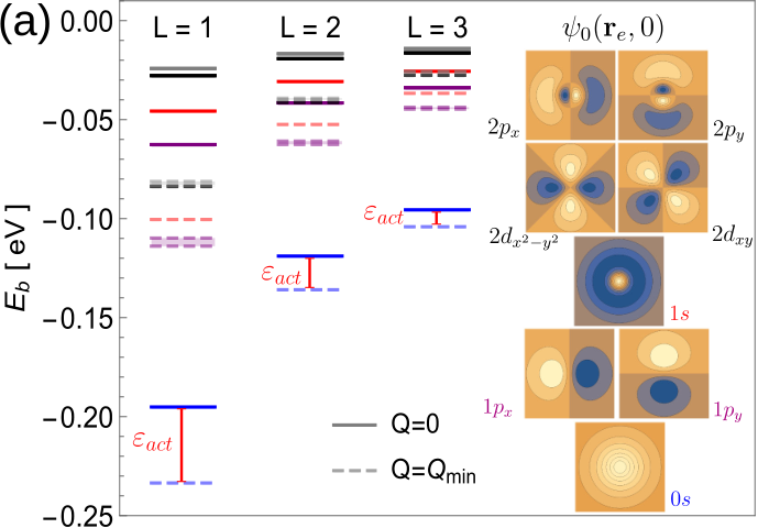
Here, we develop a mesoscale theory for the binding energies, dispersions and excited state spectra of excitons in mono-, bi-, tri-, and few-layer InSe films ($\gamma$ polytype), taking into account the strongly non-parabolic features of the valence band dispersion in these 2D materials and the influence of various encapsulation environments. In particular, we study the role of a weak inversion of the hole dispersion near the top of the valence band Zólyomi et al. 2014; Zólyomi et al. 2013; Cao et al. 2015; Trushin 2019; Skinner 2016, established in the thinnest InSe and GaSe films using angle-resolved photoemission spectroscopyHamer et al. 2019 and high field magneto-optics studiesMudd et al. 2016, and analyze the crossover of the excitons from weakly indirect to direct in momentum space, as a function of the InSe film thickness. The crossover of the exciton dispersion from indirect [$\varepsilon(Q)$=min at $Q\neq 0$] to direct [$\varepsilon(Q)$=min at $Q=0$] exciton was found at $L=7$ layers. For films with $1\leq L\leq 10$, we compute the binding energies of the excitons for hBN-encapsulated InSe films and the activation energies from the momentum-dark excitonic bound states, with the results summarized in Fig. 1.

In the analysis presented below, we describe excitons using two-particle wavefunctions, $\Psi^{\dagger}_{\mathbf{Q}}=\sum_{nm}\int d^{2}k\psi_{\mathbf{Q},nm}(\mathbf{k})a^{\dagger}_{\mathbf{k}+\mathbf{Q},n}c_{\mathbf{k},m}$, written in the wavenumber representation for the constituent electrons and holes occupying states with wavenumbers $\mathbf{k}+\mathbf{Q}$ and $\mathbf{k}$ in subbands Magorrian et al. 2018; Zultak et al. 2020 $n$ and $m$ on the conduction ($a_{\mathbf{k}+\mathbf{Q},n}$) and valence ($c_{\mathbf{k},m}$) band side of few-layer InSe film spectrum. Below, we project all electron and hole states onto the lowest subbands ($n=1$) in the film, which is justified by the much larger inter-subband energies, as compared to the exciton binding energies in the thin films (with $L\lesssim 10$ see Fig. 2). As a result, the exciton creation operator takes the approximate form $\Psi^{\dagger}_{\mathbf{Q}}=\int d^{2}k\psi_{\mathbf{Q}}(\mathbf{k})a^{\dagger}_{\mathbf{k}+\mathbf{Q},1}c_{\mathbf{k},1}$ where $\psi_{\mathbf{Q}}\equiv\psi_{\mathbf{Q},11}$. This gives the Bethe-Salpeter equationOnida et al. 2002; Jiang et al. 2007; Trolle et al. 2014; Wu et al. 2015; Deilmann and Thygesen 2019

for an effectively 2D exciton with momentum $\mathbf{Q}$ and energy $\Omega$ (the latter is a sum $\Omega=E_{g}+E_{b}$ of the gap $E_{g}$ and the binding energy $E_{b}$). Here, we use the notation $\int_{\mathbf{q}}\equiv\int\frac{\mathrm{d}^{2}q}{(2\pi)^{2}}$. The electron-hole (e-h) attraction is accounted for by the Fourier transform of the interaction potential,

designed to take into account both the dielectric polarizability of the 2DM and the dielectric environmentKeldysh 1979; Rytova 1967; Latini et al. 2015; Trolle et al. 2017 (e.g hBNGeick et al. 1966; Laturia et al. 2018, with $\kappa_{\parallel}=6.9$ and $\kappa_{z}=3.7$). For $L$-layer InSe, film thickness is $d=La_{z}$, where $a_{z}=8.32$Å is the interlayer distance and $\epsilon_{\parallel}$ and $\epsilon_{z}$ are the in- and out-of-plane permitivities of bulk InSeKuroda and Nishina 1980. The above expression takes into account $z$-dependence of the lowest electron/hole subband wave functions $\phi_{e/h,\mathbf{k}}(z)$, and $W$ is quoted for $z\geq z^{\prime}$ (for $z<z^{\prime}$, $z$ should be interchanged with $z^{\prime}$). We note that, for $L=1$ and $2$, the 2D potential $V(\mathbf{q})$ can be simplified to the Keldysh potentialKeldysh 1979; Rytova 1967; Cudazzo et al. 2011; Trolle et al. 2017,

In the above equation, $r_{*}$ is the screening length¹¹ 1 $r_{\ast}\approx L\times 7.7$ Å indicating the region dominated by the logarithmically divergent potential at lengthscales smaller than $r_{*}$ and the region dominated by the Coulombic interaction potential at distances greater than $r_{*}$. However, for $L\geq 3$, the exciton radius ($a_{exc}$) appears to be smaller than the film thickness, so that the electron/hole charge distribution along the $z$-axis in Eq.(2) needs to be taken into account in full details. To do that, we use the quantum-well approximation for the $z$-distribution of the lowest subband,Magorrian et al. 2018; García Flórez et al. 2020 $\phi_{e/h,\mathbf{k}}(z)\approx\sqrt{2/d}\cos(\pi z/d)$. We note that separating wavefunction variables and discarding higher energy subbands in Eq. (1) is applicable if the quantization energy due to confinement is much larger than the excitonic energy scale, which will be justified later by comparing the intersubband energies to the calculated exciton binding energies.

To implement numerical diagonalization of the Bethe-Salpeter equation (1), we use a basis of harmonic oscillator functions for the bound electron-hole states ²² 2 The bound electron-hole states in an exciton resemble the two-body system in a hydrogen atom. Therefore, these bound states may be well described by an atomic orbital basis set. For the sake of numerical simplicity, we use harmonic oscillator basis function which is an orthogonal Gaussian-type orbital basis., $\psi_{\mathbf{Q}}(\mathbf{k})=\sum^{N_{\mathrm{max}}}_{0\leq n_{x}\!+n_{y}}\mathcal{A}^{\mathbf{Q}}_{n_{x},n_{y}}\varphi_{n_{x}}(k_{x})\varphi_{n_{y}}(k_{y})$ where $\varphi_{n}(k)\!=\!\sqrt{\frac{\lambda}{\pi^{1/2}2^{n}n!}}(-i)^{n}\mathrm{e}^{-k^{2}\lambda^{2}/2}H_{n}(k\lambda)$ and $H_{n}(x)$ is the $n$-th Hermite polynomial. In the above described basis, the choice of the length $\lambda$ and the cutoff $N_{\mathrm{max}}$ are optimized for speeding up a converging calculation(see Appendix C for details). We also checked the performance of the developed code by comparing its results to the exact solution of the 2D hydrogen problem, aiming at $<2\%$ error as compared to the ground state energy of the Rydberg series. A software package for the implementation of numerical diagonalization of Eq. (1) with arbitrary parameters for InSe films and encapsulation environment and instructions for interested users are included in the Supplementary MaterialSM.

With this numerical setting, we solve Eq. (1) using the DFT-parameterized $\mathbf{k\cdot p}$ theory for InSe films with dispersions illustrated in Fig. 2. In particular, we used a polynomial expansion around $\Gamma$ point both for the conduction and valence bands ³³ 3 In the expansion, one has to ensure that the truncated polynomials must not allow $\varepsilon_{c}(\mathbf{k}_{e})-\varepsilon_{v}(\mathbf{k}_{h})$ smaller than the bandgap for all $\mathbf{k}_{e/h}$. computed using the GW-parameterized hybrid $\mathbf{k}\cdot\mathbf{p}$ tight-binding model (see Appendix B), $\varepsilon_{c/v}(\mathbf{k})=\sum_{i,j=0}A^{e/h}_{ij}k^{i}_{x}k^{j}_{y}$ also plotted in Figs. 2 (a)–(c). For comparison, in Fig. 2(d), we show the conduction and valence band dispersion of bulk InSe near the band edges (which are at A-point in the 3D Brillouin zone), where the inversion of $\varepsilon_{v}(\mathbf{k},k_{z})$ develops upon the increase of $z$-axis momentum, $k_{z}$ (counted from A-point).

In Fig. 3(a), we show the first eight bound states energies of the $\Gamma$-point exciton with $Q=0$ (solid line)⁴⁴ 4 The degeneracies for the non-$s$-wave states are lifted by less than $1$ meV in the tight-binding model which only has the 6-fold rotational symmetry. and the lowest-energy momentum-dark state of the exciton at $Q=Q_{\min}$ (dashed line) for $1\leq L\leq 3$. A minimum at $Q=Q_{\min}$ in the exciton dispersion for each state [Fig. 3(b)] is due to the sombrero of the $h$-band (see Fig. 2). The non-hydrogen-like energy sequenceYe et al. 2014; Zhang and Ma 2019 is due to the 2D screening of the e-h interaction in the film leading to a Keldysh-like potential for $L$=1 and 2.

To illustrate the layer-number dependence of the exciton dispersion, we compare the exciton binding energy at the $\Gamma$-point, $E_{\mathrm{b}}(0)$, and at its dispersion minimum, $E_{\mathrm{b}}(Q_{\min})$, for $L$ up to $10$ layers. In the inset in Fig. 1, we plot the activation energy, $\varepsilon_{act}$, from the dark exciton state (at $Q=Q_{\min}$) to the optically active state (at $Q=0$). We find that $\varepsilon_{act}\rightarrow 0$ at $L^{\ast}=7$, which indicates that an indirect to direct crossover for the exciton occurs before the expectation based on a single particle valence band dispersion (at $L^{\ast}=10$, see Appendix B). For completeness, we also analyzed excitons in bulk 3D InSe using bulk band dispersions shown in Fig. 2d and $V(\mathbf{q},q_{z})=-\frac{4\pi e^{2}/\epsilon_{0}}{\epsilon_{\parallel}q^{2}+\epsilon_{z}q^{2}_{z}}$. We solve the Bethe-Salpeter equation for bulk InSe using the 3D harmonic oscillator basis, and use dielectric constantsKuroda and Nishina 1980 $\epsilon_{\parallel}=10.9$, $\epsilon_{z}=9.9$ for InSe, together with the GW-computed valence band masses ($m_{v\parallel}=-5.35m_{0}$, $m_{vz}=-0.078m_{0}$) and the conduction band masses ($m_{c\parallel}/m_{0}=0.14$ and $m_{cz}/m_{0}=0.08$ where $m_{0}$ is the free electron mass) which are close to those measured in cyclotron resonance experimentsKress-Rogers et al. 1982. The examples of computed bulk exciton dispersions, $E_{3D}(\mathbf{Q},Q_{z})$ are shown in Fig. 3c. Using ($Q_{z}\approx\frac{\pi}{La_{z}}$) for the quantization of the transverse exciton motion, we find that the crossover into indirect spectrum should be expected at $L\approx 6-7$ layers, in agreement with the transition number of layers $L^{\ast}$ found in the layer dependence of the activation energy $\varepsilon_{act}$ (inset in Fig. 1). We note that the computed bulk (3D) exciton binding energy is about 30% lower than the experimentally claimed Kuroda et al. 1979; Schindlmayr 1997 values of 13-15meV. Binding energy can be increased to 14.6meV by choosing $\epsilon_{\parallel}=9.5$, $\epsilon_{z}=8.6$ (with $\sqrt{\epsilon_{z}/\epsilon_{\parallel}}=0.95$ as in Ref. Kuroda and Nishina 1980). For this reason we computed and compared the exciton spectra in the films using two choices of dielectric parameters $\epsilon_{\parallel}=10.9$,$\epsilon_{z}=9.9$ and $\epsilon_{\parallel}=9.5$,$\epsilon_{z}=8.6$. We find that in thin films $L\leq 10$ such a variation of InSe dielectric parameters has a much weaker influence on the exciton bindings than in the bulk material. These calculated binding energies compare well with the values observed in the recent experiments Zultak et al. 2020 on hBN-encapsulated thin InSe films. In summary, we present a mesoscale theory which is particularly useful for investigating the energy spectrum of a Wannier-Mott exciton in large gap semiconductors ($E_{g}\gg|E_{b}|$). Most interestingly, this theoretical framework can also be applied to study direct and indirect excitons in complex van der Waals heterostructures Fang et al. 2014; Rivera et al. 2015; *Rivera:Science351-2016; Wang et al. 2017; Ciarrocchi et al. 2018; Calman et al. 2018; Ubrig et al. 2020; Mak and Shan 2018; Fogler et al. 2014.

References

- Bhimanapati et al. (2015) G. R. Bhimanapati, Z. Lin, V. Meunier, Y. Jung, J. Cha, S. Das, D. Xiao, Y. Son, M. S. Strano, V. R. Cooper, L. Liang, S. G. Louie, E. Ringe, W. Zhou, S. S. Kim, R. R. Naik, B. G. Sumpter, H. Terrones, F. Xia, Y. Wang, J. Zhu, D. Akinwande, N. Alem, J. A. Schuller, R. E. Schaak, M. Terrones, and J. A. Robinson, ACS Nano 9, 11509 (2015).
- Qian et al. (2015) X. Qian, Y. Wang, W. Li, J. Lu, and J. Li, 2D Materials 2, 032003 (2015).
- Novoselov et al. (2016) K. S. Novoselov, A. Mishchenko, A. Carvalho, and A. H. C. Neto, Science 353, aac9439 (2016).
- Mudd et al. (2013) G. W. Mudd, S. A. Svatek, T. Ren, A. Patanè, O. Makarovsky, L. Eaves, P. H. Beton, Z. D. Kovalyuk, G. V. Lashkarev, Z. R. Kudrynskyi, et al., Advanced Materials 25, 5714 (2013).
- Lei et al. (2014) S. Lei, L. Ge, S. Najmaei, A. George, R. Kappera, J. Lou, M. Chhowalla, H. Yamaguchi, G. Gupta, R. Vajtai, A. D. Mohite, and P. M. Ajayan, ACS Nano 8, 1263 (2014).
- Brotons-Gisbert et al. (2016) M. Brotons-Gisbert, D. Andres-Penares, J. Suh, F. Hidalgo, R. Abargues, P. J. Rodríguez-Cantó, A. Segura, A. Cros, G. Tobias, E. Canadell, P. Ordejón, J. Wu, J. P. Martínez-Pastor, and J. F. Sánchez-Royo, Nano Letters 16, 3221 (2016).
- Bandurin et al. (2016) D. A. Bandurin, A. V. Tyurnina, G. L. Yu, A. Mishchenko, V. Zólyomi, S. V. Morozov, R. K. Kumar, R. V. Gorbachev, Z. R. Kudrynskyi, S. Pezzini, Z. D. Kovalyuk, U. Zeitler, K. S. Novoselov, A. Patanè, L. Eaves, I. V. Grigorieva, V. I. Fal'ko, A. K. Geim, and Y. Cao, Nature Nanotechnology 12, 223 (2016).
- Terry et al. (2018) D. J. Terry, V. Zólyomi, M. Hamer, A. V. Tyurnina, D. G. Hopkinson, A. M. Rakowski, S. J. Magorrian, N. Clark, Y. M. Andreev, O. Kazakova, K. Novoselov, S. J. Haigh, V. I. Fal’ko, and R. Gorbachev, 2D Materials 5, 041009 (2018).
- Sánchez-Royo et al. (2014) J. F. Sánchez-Royo, G. Muñoz-Matutano, M. Brotons-Gisbert, J. P. Martínez-Pastor, A. Segura, A. Cantarero, R. Mata, J. Canet-Ferrer, G. Tobias, E. Canadell, J. Marqués-Hueso, and B. D. Gerardot, Nano Research 7, 1556 (2014).
- Hamer et al. (2019) M. J. Hamer, J. Zultak, A. V. Tyurnina, V. Zólyomi, D. Terry, A. Barinov, A. Garner, J. Donoghue, A. P. Rooney, V. Kandyba, A. Giampietri, A. Graham, N. Teutsch, X. Xia, M. Koperski, S. J. Haigh, V. I. Fal’ko, R. V. Gorbachev, and N. R. Wilson, ACS Nano (2019), 10.1021/acsnano.8b08726.
- Li et al. (2014) X. Li, M.-W. Lin, A. A. Puretzky, J. C. Idrobo, C. Ma, M. Chi, M. Yoon, C. M. Rouleau, I. I. Kravchenko, D. B. Geohegan, and K. Xiao, Scientific Reports 4 (2014), 10.1038/srep05497.
- Aziza et al. (2017) Z. B. Aziza, D. Pierucci, H. Henck, M. G. Silly, C. David, M. Yoon, F. Sirotti, K. Xiao, M. Eddrief, J.-C. Girard, and A. Ouerghi, Physical Review B 96 (2017), 10.1103/physrevb.96.035407.
- Aziza et al. (2018) Z. B. Aziza, V. Zólyomi, H. Henck, D. Pierucci, M. G. Silly, J. Avila, S. J. Magorrian, J. Chaste, C. Chen, M. Yoon, K. Xiao, F. Sirotti, M. C. Asensio, E. Lhuillier, M. Eddrief, V. I. Fal'ko, and A. Ouerghi, Physical Review B 98 (2018), 10.1103/physrevb.98.115405.
- Budweg et al. (2019) A. Budweg, D. Yadav, A. Grupp, A. Leitenstorfer, M. Trushin, F. Pauly, and D. Brida, Phys. Rev. B 100, 045404 (2019).
- Rybkovskiy et al. (2011) D. V. Rybkovskiy, N. R. Arutyunyan, A. S. Orekhov, I. A. Gromchenko, I. V. Vorobiev, A. V. Osadchy, E. Y. Salaev, T. K. Baykara, K. R. Allakhverdiev, and E. D. Obraztsova, Physical Review B 84 (2011), 10.1103/physrevb.84.085314.
- Rybkovskiy et al. (2014) D. V. Rybkovskiy, A. V. Osadchy, and E. D. Obraztsova, Phys. Rev. B 90 (2014), 10.1103/physrevb.90.235302.
- Zólyomi et al. (2013) V. Zólyomi, N. D. Drummond, and V. I. Fal'ko, Physical Review B 87 (2013), 10.1103/physrevb.87.195403.
- Zólyomi et al. (2014) V. Zólyomi, N. D. Drummond, and V. I. Fal’ko, Phys. Rev. B 89, 205416 (2014).
- Zhou et al. (2017) M. Zhou, R. Zhang, J. Sun, W.-K. Lou, D. Zhang, W. Yang, and K. Chang, Phys. Rev. B 96 (2017), 10.1103/physrevb.96.155430.
- Zhou et al. (2019) M. Zhou, D. Zhang, S. Yu, Z. Huang, Y. Chen, W. Yang, and K. Chang, Phys. Rev. B 99, 155402 (2019).
- Sun et al. (2018) Y. Sun, S. Luo, X.-G. Zhao, K. Biswas, S.-L. Li, and L. Zhang, Nanoscale 10, 7991 (2018).
- Magorrian et al. (2016) S. J. Magorrian, V. Zólyomi, and V. I. Fal'ko, Phys. Rev. B 94 (2016), 10.1103/physrevb.94.245431.
- Cao et al. (2015) T. Cao, Z. Li, and S. G. Louie, Phys. Rev. Lett. 114, 236602 (2015).
- Trushin (2019) M. Trushin, Phys. Rev. B 99, 205307 (2019).
- Skinner (2016) B. Skinner, Phys. Rev. B 93, 235110 (2016).
- Mudd et al. (2016) G. W. Mudd, M. R. Molas, X. Chen, V. Zólyomi, K. Nogajewski, Z. R. Kudrynskyi, Z. D. Kovalyuk, G. Yusa, O. Makarovsky, L. Eaves, M. Potemski, V. I. Fal’ko, and A. Patanè, Sci. Rep. 6 (2016), 10.1038/srep39619.
- Magorrian et al. (2018) S. J. Magorrian, A. Ceferino, V. Zólyomi, and V. I. Fal’ko, Phys. Rev. B 97, 165304 (2018).
- Zultak et al. (2020) J. Zultak, S. J. Magorrian, M. Koperski, A. Garner, M. J. Hamer, E. Tóvári, K. S. Novoselov, A. A. Zhukov, Y. Zou, N. R. Wilson, S. J. Haigh, A. V. Kretinin, V. I. Fal’ko, and R. Gorbachev, Nature Communications 11 (2020), 10.1038/s41467-019-13893-w.
- Onida et al. (2002) G. Onida, L. Reining, and A. Rubio, Rev. Mod. Phys. 74, 601 (2002).
- Jiang et al. (2007) J. Jiang, R. Saito, G. G. Samsonidze, A. Jorio, S. G. Chou, G. Dresselhaus, and M. S. Dresselhaus, Phys. Rev. B 75 (2007), 10.1103/physrevb.75.035407.
- Trolle et al. (2014) M. L. Trolle, G. Seifert, and T. G. Pedersen, Phys. Rev. B 89, 235410 (2014).
- Wu et al. (2015) F. Wu, F. Qu, and A. H. MacDonald, Phys. Rev. B 91, 075310 (2015).
- Deilmann and Thygesen (2019) T. Deilmann and K. S. Thygesen, 2D Mater. 6, 035003 (2019).
- Keldysh (1979) L. V. Keldysh, Soviet Journal of Experimental and Theoretical Physics Letters 29, 658 (1979).
- Rytova (1967) N. S. Rytova, Moscow Univ. Phys. Bull. 3, 18 (1967).
- Latini et al. (2015) S. Latini, T. Olsen, and K. S. Thygesen, Phys. Rev. B 92, 245123 (2015).
- Trolle et al. (2017) M. L. Trolle, T. G. Pedersen, and V. Véniard, Sci. Rep. 7, 39844 (2017).
- Geick et al. (1966) R. Geick, C. H. Perry, and G. Rupprecht, Phys. Rev. 146, 543 (1966).
- Laturia et al. (2018) A. Laturia, M. L. V. de Put, and W. G. Vandenberghe, npj 2D Mater. Appl. 2 (2018), 10.1038/s41699-018-0050-x.
- Kuroda and Nishina (1980) N. Kuroda and Y. Nishina, Solid State Commun. 34, 481 (1980).
- Cudazzo et al. (2011) P. Cudazzo, I. V. Tokatly, and A. Rubio, Phys. Rev. B 84 (2011), 10.1103/physrevb.84.085406.
- (42) Å.
- García Flórez et al. (2020) F. García Flórez, L. D. A. Siebbeles, and H. T. C. Stoof, arXiv e-prints , arXiv:2002.05921 (2020), arXiv:2002.05921 [cond-mat.mes-hall] .
- (44) The bound electron-hole states in an exciton resemble the two-body system in a hydrogen atom. Therefore, these bound states may be well described by an atomic orbital basis set. For the sake of numerical simplicity, we use harmonic oscillator basis function which is an orthogonal Gaussian-type orbital basis.
- (45) See Supplemental Material at […] for the software package. The instruction is included in the file.
- (46) In the expansion, one has to ensure that the truncated polynomials must not allow smaller than the bandgap for all .
- (47) The degeneracies for the non--wave states are lifted by less than meV in the tight-binding model which only has the 6-fold rotational symmetry.
- Ye et al. (2014) Z. Ye, T. Cao, K. O’Brien, H. Zhu, X. Yin, Y. Wang, S. G. Louie, and X. Zhang, Nature 513, 214 (2014).
- Zhang and Ma (2019) J.-Z. Zhang and J.-Z. Ma, J. Phys. Condens. Matter 31, 105702 (2019).
- Kress-Rogers et al. (1982) E. Kress-Rogers, R. Nicholas, J. Portal, and A. Chevy, Solid State Communications 44, 379 (1982).
- Kuroda et al. (1979) N. Kuroda, Y. Nishina, H. Hori, and M. Date, Journal of the Physical Society of Japan 47, 1373 (1979), https://doi.org/10.1143/JPSJ.47.1373 .
- Schindlmayr (1997) A. Schindlmayr, European Journal of Physics 18, 374 (1997).
- Fang et al. (2014) H. Fang, C. Battaglia, C. Carraro, S. Nemsak, B. Ozdol, J. S. Kang, H. A. Bechtel, S. B. Desai, F. Kronast, A. A. Unal, G. Conti, C. Conlon, G. K. Palsson, M. C. Martin, A. M. Minor, C. S. Fadley, E. Yablonovitch, R. Maboudian, and A. Javey, Proceedings of the National Academy of Sciences 111, 6198 (2014).
- Rivera et al. (2015) P. Rivera, J. R. Schaibley, A. M. Jones, J. S. Ross, S. Wu, G. Aivazian, P. Klement, K. Seyler, G. Clark, N. J. Ghimire, J. Yan, D. G. Mandrus, W. Yao, and X. Xu, Nature Communications 6 (2015), 10.1038/ncomms7242.
- Rivera et al. (2016) P. Rivera, K. L. Seyler, H. Yu, J. R. Schaibley, J. Yan, D. G. Mandrus, W. Yao, and X. Xu, Science 351, 688 (2016).
- Wang et al. (2017) Z. Wang, Y.-H. Chiu, K. Honz, K. F. Mak, and J. Shan, Nano Letters 18, 137 (2017).
- Ciarrocchi et al. (2018) A. Ciarrocchi, D. Unuchek, A. Avsar, K. Watanabe, T. Taniguchi, and A. Kis, Nature Photonics 13, 131 (2018).
- Calman et al. (2018) E. V. Calman, M. M. Fogler, L. V. Butov, S. Hu, A. Mishchenko, and A. K. Geim, Nature Communications 9 (2018), 10.1038/s41467-018-04293-7.
- Ubrig et al. (2020) N. Ubrig, E. Ponomarev, J. Zultak, D. Domaretskiy, V. Zólyomi, D. Terry, J. Howarth, I. Gutiérrez-Lezama, A. Zhukov, Z. R. Kudrynskyi, Z. D. Kovalyuk, A. Patané, T. Taniguchi, K. Watanabe, R. V. Gorbachev, V. I. Fal’ko, and A. F. Morpurgo, Nature Materials (2020), 10.1038/s41563-019-0601-3.
- Mak and Shan (2018) K. F. Mak and J. Shan, Nature Nanotechnology 13, 974 (2018).
- Fogler et al. (2014) M. M. Fogler, L. V. Butov, and K. S. Novoselov, Nature Communications 5, 4555 (2014), arXiv:1404.1418 [cond-mat.mes-hall] .
- Li and Appelbaum (2015) P. Li and I. Appelbaum, Phys. Rev. B 92, 195129 (2015).
- Ruiz-Tijerina et al. (2018) D. A. Ruiz-Tijerina, M. Danovich, C. Yelgel, V. Zólyomi, and V. I. Fal’ko, Phys. Rev. B 98, 035411 (2018).
- Fiorentini and Baldereschi (1995) V. Fiorentini and A. Baldereschi, Phys. Rev. B 51, 17196 (1995).
- Johnson and Ashcroft (1998) K. A. Johnson and N. W. Ashcroft, Phys. Rev. B 58, 15548 (1998).
- Bernstein et al. (2002) N. Bernstein, M. J. Mehl, and D. A. Papaconstantopoulos, Phys. Rev. B 66, 075212 (2002).
- Kotani et al. (2007) T. Kotani, M. van Schilfgaarde, and S. V. Faleev, Physical Review B 76, 165106 (2007).
- Pashov et al. (2020) D. Pashov, S. Acharya, W. R. Lambrecht, J. Jackson, K. D. Belashchenko, A. Chantis, F. Jamet, and M. van Schilfgaarde, Computer Physics Communications 249, 107065 (2020).
- Li et al. (2018) Y. Li, T. Wang, M. Wu, T. Cao, Y. Chen, R. Sankar, R. K. Ulaganathan, F. Chou, C. Wetzel, C.-Y. Xu, S. G. Louie, and S.-F. Shi, 2D Materials 5, 021002 (2018).
- Song et al. (2018) C. Song, F. Fan, N. Xuan, S. Huang, G. Zhang, C. Wang, Z. Sun, H. Wu, and H. Yan, ACS Applied Materials & Interfaces 10, 3994 (2018).
- Rigoult et al. (1980) J. Rigoult, A. Rimsky, and A. Kuhn, Acta Crystallographica B 36, 916 (1980).
- Camassel et al. (1978) J. Camassel, P. Merle, H. Mathieu, and A. Chevy, Physical Review B 17, 4718 (1978).
- Chadi and Cohen (1973) D. J. Chadi and M. L. Cohen, Phys. Rev. B 8, 5747 (1973).
- Cunningham (1974) S. L. Cunningham, Phys. Rev. B 10, 4988 (1974).
- Monkhorst and Pack (1976) H. J. Monkhorst and J. D. Pack, Phys. Rev. B 13, 5188 (1976).
- Magalhães (2014) A. L. Magalhães, Journal of Chemical Education 91, 2124 (2014), https://doi.org/10.1021/ed500437a .