Finite Element Approximation and Analysis of a Viscoelastic Scalar Wave Equation with Internal Variable FormulationsJournal: Journal of Computational and Applied Mathematics

Yongseok Jang Email: jang@cerfacs.fr Corresponding author: Corresponding author Note: Jang gratefully acknowledges the support of a scholarship from Brunel University London. Address: CERFACS, 42 Avenue Gaspard Coriolis, 31057, Toulouse, France. Simon Shaw Email: simon.shaw@brunel.ac.uk Address: Department of Mathematics, Brunel University London, Uxbridge UB8 3PH, UK.

Abstract

We consider linear scalar wave equations with a hereditary integral term of the kind used to model viscoelastic solids. The kernel in this Volterra integral is a sum of decaying exponentials (The so-called Maxwell, or Zener model) and this allows the introduction of one of two types of families of internal variables, each of which evolve according to an ordinary differential equation (ODE). There is one such ODE for each decaying exponential, and the introduction of these ODEs means that the Volterra integral can be removed from the governing equation. The two types of internal variable are distinguished by whether the unknown appears in the Volterra integral, or whether its time derivative appears; we call the resulting problems the displacement and velocity forms. We define fully discrete formulations for each of these forms by using continuous Galerkin finite element approximations in space and an implicit ‘Crank-Nicolson’ type of finite difference method in time. We prove stability and a priori bounds, and using the FEniCS environment, https://fenicsproject.org/ (The FEniCS project version 1.5, Archive of Numerical Software, 3 (100), 9–23, 2015.) give some numerical results. These bounds do not require Grönwall’s inequality and so can be regarded to be of high quality, allowing confidence in long time integration without an a priori exponential build up of error. As far as we are aware this is the first time that these two formulations have been described together with accompanying proofs of such high quality stability and error bounds. The extension of the results to vector-valued viscoelasticity problems is straightforward and summarised at the end. The numerical results are reproducible by acquiring the python sources from https://github.com/Yongseok7717, or by running a custom built docker container (instructions are given).

Keywords:

viscoelasticity, finite element method, internal variables, a priori estimates

1 Introduction

Materials that exhibit both elastic and viscous response to imposed load and/or deformation are called viscoelastic. Typical examples of such solid materials are amorphous polymers, soft biotissue, metals at high temperatures and even concrete [1]. The mathematical description of the dynamic response of these materials uses a momentum balance law to relate external forces, $f$ , to acceleration, $\ddot{u}$ , and stress divergence, $\nabla\cdot\mathchoice{\hbox to0.0pt{{$\underline{{\hbox to4.5713pt{}}}$\hss}}}{\hbox to0.0pt{{$\underline{{\hbox to4.5713pt{}}}$\hss}}}{\hbox to0.0pt{{$\underline{{\hbox to3.70715pt{}}}$\hss}}}{\hbox to0.0pt{{$\underline{{\hbox to3.26068pt{}}}$\hss}}}\sigma$ . A faithful mathematical model of this physical set-up would require the introduction of a vector-valued partial differential equation as in elastodynamics (see e.g. [2, 3]) but we restrict ourselves here to a scalar analogue to keep the exposition as simple as possible (but we use the terminology of solid mechanics).

So, with that in mind, once boundary and initial data are specified, the physical problem is exemplified by the following mathematical model: find $u\colon[0,T]\times\Omega\to\mathbb{R}$ such that

$\displaystyle\rho\ddot{u}-\nabla\cdot\mathchoice{\hbox to0.0pt{{$\underline{{\hbox to4.5713pt{}}}$\hss}}}{\hbox to0.0pt{{$\underline{{\hbox to4.5713pt{}}}$\hss}}}{\hbox to0.0pt{{$\underline{{\hbox to3.70715pt{}}}$\hss}}}{\hbox to0.0pt{{$\underline{{\hbox to3.26068pt{}}}$\hss}}}\sigma=f$	in	$\displaystyle(0,T]\times\Omega,$	(1.1)
$\displaystyle u=0$	on	$\displaystyle[0,T]\times\Gamma_{D},$	(1.2)
$\displaystyle\mathchoice{\hbox to0.0pt{{$\underline{{\hbox to4.5713pt{}}}$\hss}}}{\hbox to0.0pt{{$\underline{{\hbox to4.5713pt{}}}$\hss}}}{\hbox to0.0pt{{$\underline{{\hbox to3.70715pt{}}}$\hss}}}{\hbox to0.0pt{{$\underline{{\hbox to3.26068pt{}}}$\hss}}}\sigma\cdot\mathchoice{\hbox to0.0pt{{$\underline{{\hbox to4.8019pt{}}}$\hss}}}{\hbox to0.0pt{{$\underline{{\hbox to4.8019pt{}}}$\hss}}}{\hbox to0.0pt{{$\underline{{\hbox to3.95467pt{}}}$\hss}}}{\hbox to0.0pt{{$\underline{{\hbox to3.5232pt{}}}$\hss}}}n=g_{N}$	on	$\displaystyle[0,T]\times\Gamma_{N},$	(1.3)
$\displaystyle u=u_{0}$	on	$\displaystyle\{0\}\times\Omega,$	(1.4)
$\displaystyle\dot{u}=w_{0}$	on	$\displaystyle\{0\}\times\Omega,$	(1.5)

where we refer to $\mathchoice{\hbox to0.0pt{{$\underline{{\hbox to4.5713pt{}}}$\hss}}}{\hbox to0.0pt{{$\underline{{\hbox to4.5713pt{}}}$\hss}}}{\hbox to0.0pt{{$\underline{{\hbox to3.70715pt{}}}$\hss}}}{\hbox to0.0pt{{$\underline{{\hbox to3.26068pt{}}}$\hss}}}\sigma$ as the stress (and describe it more fully below); $\Omega$ is an open bounded polytopic domain in $\mathbb{R}^{d}$ with constant mass density $\rho$ ; $\Gamma_{D}$ and $\Gamma_{N}$ are the ‘Dirichlet’ and ‘Neumann’ boundaries and $T>0$ is a final time. As usual $\Gamma_{D}$ and $\Gamma_{N}$ are disjoint and we will assume that the surface measure of $\Gamma_{D}$ is strictly positive. Note that we use overdots to denote time differentiation so that $\dot{u}:=\frac{\partial u}{\partial t}$ and $\ddot{u}:=\frac{\partial^{2}u}{\partial t^{2}}$ . In classical continuum mechanics, the physical model is defined with a displacement vector so the stress is a second order tensor and is defined by a constitutive relationship with the strain tensor. Hence, in general, the linear viscoelastic dynamic equation is a vector-valued PDE of which the above is a scalar analogue. However, (1.1) is not only a scalar analogue but also represents the mathematical model of viscoelastic materials subjected to antiplane shear response. Antiplane strain, for instance, allows us to reduce the second order tensor to a vector so that the viscoelastic antiplane model in 3D can be dealt with by the scalar wave problem in 2D (see e.g. [4, 5, 6]).

The viscoelasticity literature contains a large number of rheological (spring and dashpot) based phenomenological models (e.g. the Maxwell, Voigt, Kelvin-Voigt, generalised Maxwell, $\ldots$ , models — see [2, 7] for more details) as well as models based on the fractional calculus, referred to as ‘power law’ models in [8]. The spring and dashpot models are the ones of interest here because they give rise to stress-strain constitutive laws that can be described by Volterra kernels of sums of decaying exponentials. This, in turn, makes them much better suited to numerical approximation than the fractional calculus models in the sense that the entire solution history need not be stored, and there is no weak singularity in the kernel. We will return to the first point below, but first recall the form of these constitutive laws from [2] in the following two equivalent (integrate by parts) forms:

	$\displaystyle\mathchoice{\hbox to0.0pt{{$\underline{{\hbox to4.5713pt{}}}$\hss}}}{\hbox to0.0pt{{$\underline{{\hbox to4.5713pt{}}}$\hss}}}{\hbox to0.0pt{{$\underline{{\hbox to3.70715pt{}}}$\hss}}}{\hbox to0.0pt{{$\underline{{\hbox to3.26068pt{}}}$\hss}}}\sigma(t)=$	$\displaystyle D\varphi(0)\nabla u(t)-\int^{t}_{0}D\varphi_{s}(t-s)\nabla u(s)ds,$		(1.6)
	$\displaystyle=$	$\displaystyle D\varphi(t)\nabla u(0)+\int^{t}_{0}D\varphi(t-s)\nabla\dot{u}(s)ds,$		(1.7)

where $D$ is a positive constant, $\varphi(t)$ is a stress relaxation function and $\varphi_{s}(t-s):=\frac{\partial}{\partial s}\varphi(t-s)$ . Now we can complete our model problem by defining the stress relaxation function $\varphi(t)$ and then substituting for $\mathchoice{\hbox to0.0pt{{$\underline{{\hbox to4.5713pt{}}}$\hss}}}{\hbox to0.0pt{{$\underline{{\hbox to4.5713pt{}}}$\hss}}}{\hbox to0.0pt{{$\underline{{\hbox to3.70715pt{}}}$\hss}}}{\hbox to0.0pt{{$\underline{{\hbox to3.26068pt{}}}$\hss}}}\sigma$ in (1.1) and (1.3). The generalised Maxwell model for a viscoelastic solid produces the following stress relaxation function (see e.g. [8]),

\varphi(t)=\varphi_{0}+\sum_{q=1}^{N_{\varphi}}\varphi_{q}e^{-t/\tau_{q}},

(1.8)

with $N_{\varphi}\in\mathbb{N}$ , positive delay times $\{\tau_{q}\}^{N_{\varphi}}_{q=1}$ and positive coefficients $\{\varphi_{q}\}^{N_{\varphi}}_{q=0}$ which we can assume to be normalised so that $\varphi(0)=1$ .

The form (1.8) permits us to deal with the Volterra integrals in (1.6) and (1.7) in a way that avoids any reference to the past ‘history’ of the solution. In this approach, detailed later in (2.3), (2.4), (2.5), (2.9) and (2.10), the stress $\mathchoice{\hbox to0.0pt{{$\underline{{\hbox to4.5713pt{}}}$\hss}}}{\hbox to0.0pt{{$\underline{{\hbox to4.5713pt{}}}$\hss}}}{\hbox to0.0pt{{$\underline{{\hbox to3.70715pt{}}}$\hss}}}{\hbox to0.0pt{{$\underline{{\hbox to3.26068pt{}}}$\hss}}}\sigma$ is defined by using, in place of the Volterra integral, ‘hidden’ or internal variables (e.g. [2, 9]) that evolve following an ordinary differential equation. Each of (1.6) and (1.7) gives rise to different internal variables and so will be considered separately to give two formulations: the displacement form and the velocity form. For each of these we will approximate the solution and the internal variables using the standard continuous Galerkin Finite Element Method (CGFEM) to discretise in space, and a second order implicit Crank-Nicolson finite difference method for the time discretisation.

The plan of the paper is as follows. In Section 2 we introduce the displacement form of the problem in Subsection 2.1, and the velocity form in Subsection 2.2. The fully discrete approximations are then given in Sections 3 (displacement form) and 4 (velocity form) where we prove stability and a priori error estimates. Grönwall’s lemma (e.g. [10, 11]) is not used for these proofs and so the constants in these bounds do not grow exponentially with time and we can, therefore, have confidence in these schemes for long-time integration. The Grönwall lemma allows for some simplification of analysis (see e.g. [3, 12, 13]), and to circumvent it requires some effort. Here we rely on assumptions that arise from the physical character and properties of the problem, and then, to achieve the sharper bounds, our proofs use some long and technical calculations and details. These are sometimes omitted or just sketched out where it aids presentation of the main ideas and specific arguments. In Section 5 we use the FEniCS environment (see [14], https://fenicsproject.org/) to give the results of some numerical experiments, and explain how our software can be acquired and the results reproduced. We finish in Section 6 with some general comments. We also note that the results herein are presented in expanded form in [15].

In terms of context we note that for the integral form of the quasistatic (i.e. where $\rho\ddot{u}$ is neglected) version of this viscoelasticity problem estimates that avoid Grönwall’s inequality were given in [16, 17, 18, 19]. For the dynamic problem we refer to DG-in-time, and DG-in-space methods in [20, 21] — only the first of these avoided the Grönwall lemma, whereas the second is similar to what we refer to as the ‘displacement formulation’ below. Of these, [20, 19, 21] used space-time finite element formulations. More generally, the integral form of the dynamic problem has been studied widely in, for example, [22, 23]. The contribution of this paper is to give two formulations of the dynamic problem using internal variables, and give accompanying stability and error estimates that completely avoid the Grönwall inequality. As far as we are aware equivalent analyses are not currently available. In terms of the well-posedness of problems of this type we refer to the well-known paper [24].

We introduce and use some standard notations so that $L_{p}(\Omega),H^{s}(\Omega)$ and $W^{s}_{p}(\Omega)$ denote the usual Lebesgue, Hilbert and Sobolev spaces. For any Banach space $X$ , $\lVert\cdot\rVert_{X}$ is the $X$ norm. For example, $\left\lVert\cdot\right\rVert_{L_{2}(\Omega)}$ is the $L_{2}$ norm induced by the $L_{2}$ inner product which we denote by $(\cdot,\cdot)$ for the entire domain but for $S\subset\bar{\Omega}$ , $(\cdot,\cdot)_{L_{2}(S)}$ is the $L_{2}$ inner product over $S$ . In the case of time dependent functions, we expand this notation such that if $f\in L_{p}(0,T;X)$ for some Banach space $X$ , we define $\lVert f\rVert_{L_{p}(0,t_{0};X)}$ to be the $L_{p}(0,t_{0})$ norm of $\lVert f(t)\rVert_{X}$ . We also use the same notation for vector valued functions in Section 6. Lastly in this section, and for use later, we recall the trace inequality,

\displaystyle\lVert v\rVert_{L_{2}(\partial\Omega)}

\displaystyle\leq C\left\lVert v\right\rVert_{H^{1}(\Omega)}\textrm{ for any }v\in H^{1}(\Omega),

(1.9)

where $C$ is a positive constant depending only on $\Omega$ and its boundary $\partial\Omega$ .

2 Weak formulations

Our first step is to define the test space $V$ ,

\displaystyle V=\left\{v\in H^{1}(\Omega)\ |\ v=0\ \textrm{ on }{\Gamma_{D}}\right\},

and then, multiplying (1.1) by $v\in V$ , integrating by parts and using the boundary data gives, in a standard way, that

\displaystyle\left(\rho\ddot{u}(t),v\right)+(\sigma(t),\nabla v)=F_{d}(t;v)

(2.1)

for all $v\in V$ where the time dependent linear form $F_{d}$ is defined by

F_{d}(t;v)=\left(f(t),v\right)+(g_{N}(t),v)_{L_{2}(\Gamma_{N})}.

(2.2)

We now need to substitute for the stress using either the displacement or velocity forms.

2.1 Displacement form

Recalling (1.6) and (1.8) we write

\displaystyle\mathchoice{\hbox to0.0pt{{$\underline{{\hbox to4.5713pt{}}}$\hss}}}{\hbox to0.0pt{{$\underline{{\hbox to4.5713pt{}}}$\hss}}}{\hbox to0.0pt{{$\underline{{\hbox to3.70715pt{}}}$\hss}}}{\hbox to0.0pt{{$\underline{{\hbox to3.26068pt{}}}$\hss}}}\sigma(t)=D\nabla\left(u(t)-\sum_{{q}=1}^{N_{\varphi}}\psi_{q}(t)\right),

(2.3)

where, for $1\leq{q}\leq N_{\varphi}$ , the internal variables are defined by

\displaystyle\psi_{q}(t):=\frac{\varphi_{q}}{\tau_{q}}\int^{t}_{0}e^{-(t-s)/\tau_{q}}u(s)\ ds,

(2.4)

and satisfy the following ODEs,

\displaystyle\dot{\psi}_{q}(t)=\frac{\varphi_{q}}{\tau_{q}}u(t)-\frac{1}{\tau_{q}}\psi_{q}(t)\qquad\textrm{for }q=1,2,\ldots,N_{\varphi},

(2.5)

with $\psi_{q}(0)=0$ . Our weak formulation (2.1) can now be written as

\displaystyle\left(\rho\ddot{u}(t),v\right)+a(u(t),v)-\sum_{q=1}^{N_{\varphi}}a(\psi_{q}(t),v)=F_{d}(t;v)\qquad\forall v\in V.

(2.6)

In this the symmetric bilinear form $a\colon V\times V\to\mathbb{R}$ is defined by $a(w,v)=\left(D\nabla w,\nabla v\right)$ and is easily shown to be continuous on $V$ . Moreover, it follows from our assumption on $\Gamma_{D}$ that it is also coercive on $V$ , [25], and so the energy norm defined by $\|v\|_{V}:=\sqrt{a(v,v)}$ , for $v\in V$ , satisfies $\kappa\left\lVert v\right\rVert_{H^{1}(\Omega)}^{2}\leq\left\lVert v\right\rVert_{V}^{2}\leq D\left\lVert v\right\rVert_{H^{1}(\Omega)}^{2}$ for a positive constant $\kappa$ . Thus $(V,a(\cdot,\cdot))$ is a Hilbert space equivalent to $(H^{1}(\Omega),(\cdot,\cdot)_{H^{1}(\Omega)})$ .

We use this bilinear form, or energy inner product, to enforce each internal variable ODE, and then arrive at the following weak problem.

(P1) Find $(0,T]\to V$ maps $u$ , $\psi_{1}$ , $\psi_{2},\ldots,\psi_{N_{\varphi}}$ such that

	$\displaystyle\left(\rho\ddot{u}(t),v\right)+a(u(t),v)-\sum_{q=1}^{N_{\varphi}}a(\psi_{q}(t),v)$	$\displaystyle=F_{d}(t;v)\qquad$		$\displaystyle\forall v\in V,$		(2.7)
	$\displaystyle\tau_{q}a(\dot{\psi}_{q}(t),v)+a(\psi_{q}(t),v)$	$\displaystyle=\varphi_{q}a(u(t),v)\qquad$		$\displaystyle\forall v\in V,\ q=1,\ldots,N_{\varphi}$		(2.8)

with $u(0)=u_{0},$ $\dot{u}(0)=w_{0}$ and $\psi_{q}(0)=0,\ \forall{q}\in\{1,\ldots,N_{\varphi}\}$ .

2.2 Velocity form

On the other hand, using (1.7) and (1.8) with the velocity form of internal variable given by

\zeta_{q}(t)=\int^{t}_{0}\varphi_{q}e^{-(t-s)/\tau_{q}}\dot{u}(s)\ ds,

(2.9)

for each $q=1,\ldots,N_{\varphi}$ , we have

\dot{\zeta}_{q}(t)+\frac{1}{\tau_{q}}\zeta_{q}(t)=\varphi_{q}\dot{u}(t)\qquad\textrm{for }q=1,2,\ldots,N_{\varphi},

(2.10)

with $\zeta_{q}(0)=0$ . Noticing that $\psi_{q}(t)=\varphi_{q}u(t)-\varphi_{q}e^{-t/\tau_{q}}u_{0}-\zeta_{q}(t)$ (integrate by parts) and recalling that $\varphi(0)=1$ we can observe that

u(t)-\sum_{{q}=1}^{N_{\varphi}}\psi_{q}(t)=\varphi_{0}u(t)+\sum_{{q}=1}^{N_{\varphi}}\Big(\varphi_{q}e^{-t/\tau_{q}}u_{0}+\zeta_{q}(t)\Big).

Using this in (2.3), substituting the result into (2.1) and incorporating (2.10), gives the weak problem for the velocity form.

(P2) Find $(0,T]\to V$ maps $u$ , $\zeta_{1}$ , $\zeta_{2},\ldots,\zeta_{N_{\varphi}}$ such that

	$\displaystyle\left(\rho\ddot{u}(t),v\right)+\varphi_{0}a(u(t),v)+\sum_{q=1}^{N_{\varphi}}a(\zeta_{q}(t),v)=F_{v}(t;v)\qquad$	$\displaystyle\forall v\in V,$		(2.11)
	$\displaystyle\tau_{q}a(\dot{\zeta}_{q}(t),v)+a(\zeta_{q}(t),v)=\tau_{q}\varphi_{q}a(\dot{u}(t),v)\qquad$	$\displaystyle\forall v\in V,\ q=1,\ldots,N_{\varphi},$		(2.12)

with $u(0)=u_{0},$ $\dot{u}(0)=w_{0}$ , $\zeta_{q}(0)=0,\ \forall{q}$ and $F_{v}(t;v)=F_{d}(t;v)-\sum\limits_{{q}=1}^{N_{\varphi}}\varphi_{q}e^{-t/\tau_{q}}a(u_{0},v)$ .

We now move to the fully discrete schemes for (P1) in the next section and for (P2) in Section 4.

3 Fully discrete formulation: Displacement form

Let $V^{h}\subset V$ be a conforming finite element space built with continuous piecewise Lagrange basis functions with respect to an underlying quasi-uniform mesh with mesh-size characterised by $h$ . We write $t_{n}=n\Delta t$ with time step $\Delta t=T/N$ for $N\in\mathbb{N}$ , and denote the fully discrete approximations to $u$ and $\dot{u}$ by $u(t_{n})=u^{n}\approx Z_{h}^{n}\in V^{h}$ and $\dot{u}(t_{n})=\dot{u}^{n}\approx W_{h}^{n}\in V^{h}$ . Furthermore, we will use the following approximations,

\frac{\ddot{u}(t_{n+1})+\ddot{u}(t_{n})}{2}\approx\frac{W^{n+1}_{h}-W^{n}_{h}}{\Delta t}\qquad\textrm{ and }\qquad\frac{u(t_{n+1})+u(t_{n})}{2}\approx\frac{Z^{n+1}_{h}+Z^{n}_{h}}{2},

and will impose the relation

\frac{W^{n+1}_{h}+W^{n}_{h}}{2}=\frac{Z^{n+1}_{h}-Z^{n}_{h}}{\Delta t}

(3.1)

in our fully discrete schemes.

Our fully discrete formulation for (P1) is:

$\mathrm{(\mathbf{P1})}^{h}$ Find $Z^{n}_{h}$ , $W^{n}_{h}$ , ${\Psi}_{h1}^{n}$ , ${\Psi}_{h2}^{n},\ldots,$ ${\Psi}_{hN_{\varphi}}^{n}\in V^{h}$ for $n=0,\ldots,N$ such that (3.1) holds along with:

$\displaystyle\left(\rho\frac{W^{n+1}_{h}-W^{n}_{h}}{\Delta t},v\right)+a\left(\frac{Z_{h}^{n+1}+Z_{h}^{n}}{2},v\right)-$	$\displaystyle\sum\limits_{q=1}^{N_{\varphi}}a\left(\frac{{\Psi}_{hq}^{n+1}+{\Psi}_{hq}^{n}}{2},v\right)$
	$\displaystyle=\frac{F_{d}(t_{n+1};v)+F_{d}(t_{n};v)}{2},$	(3.2)
$\displaystyle\tau_{q}a\left(\frac{{\Psi}_{hq}^{n+1}-{\Psi}_{hq}^{n}}{\Delta t},v\right)+a\left(\frac{{\Psi}_{hq}^{n+1}+{\Psi}_{hq}^{n}}{2},v\right)$	$\displaystyle=\varphi_{q}a\left(\frac{Z_{h}^{n+1}+Z_{h}^{n}}{2},v\right)\textrm{ for each }{q},$	(3.3)
$\displaystyle a(Z_{h}^{0},{v})$	$\displaystyle=a({u_{0}},{v}),$	(3.4)
$\displaystyle\left(W^{0}_{h},v\right)$	$\displaystyle=\left(w_{0},v\right),$	(3.5)
$\displaystyle{\Psi}_{hq}^{0}$	$\displaystyle=0\qquad\textrm{for each }q,$	(3.6)

each for all $v\in V^{h}$ . It follows immediately that $\left\lVert Z^{0}_{h}\right\rVert_{V}\leq\left\lVert u_{0}\right\rVert_{V}$ and $\textrm{and}\left\lVert W^{0}_{h}\right\rVert_{L_{2}(\Omega)}\leq\left\lVert w_{0}\right\rVert_{L_{2}(\Omega)}$ , and we have the following stability estimate.

Theorem 3.1.

Suppose $f\in C(0,T;L_{2}(\Omega))$ , $g_{N}\in H^{1}(0,T;L_{2}(\Gamma_{N}))\cap C(0,T;L_{2}(\Gamma_{N}))$ and $u_{0}\in H^{1}(\Omega)$ , then $\mathrm{(\mathbf{P1})}^{h}$ has a unique solution. Moreover, there exists a positive constant $C$ depending on $\Omega,\ \partial\Omega$ the sets $\{\varphi_{q}\}_{q=0}^{N_{\varphi}}$ and $\{\tau_{q}\}_{q=1}^{N_{\varphi}}$ , but independent of $h$ , $\Delta t$ , $T$ and the exact and numerical solutions, such that

\frac{\rho}{2}\max_{0\leq n\leq N}\left\lVert W^{n}_{h}\right\rVert_{L_{2}(\Omega)}^{2}+\frac{\varphi_{0}}{4}\max_{0\leq n\leq N}\left\lVert Z^{n}_{h}\right\rVert_{V}^{2}\\ +\sum_{q=1}^{N_{\varphi}}\frac{\varphi_{0}}{2\varphi_{q}^{2}N_{\varphi}+\varphi_{q}\varphi_{0}}\max_{0\leq n\leq N}\left\lVert{\Psi}^{n}_{hq}\right\rVert_{V}^{2}+\sum_{q=1}^{N_{\varphi}}\sum_{n=0}^{N-1}\frac{2\tau_{q}}{\Delta t\varphi_{q}}\left\lVert{\Psi}^{n+1}_{hq}-{\Psi}^{n}_{hq}\right\rVert_{V}^{2}\\ \leq CT^{2}\bigg(\left\lVert w_{0}\right\rVert_{L_{2}(\Omega)}^{2}+\left\lVert u_{0}\right\rVert_{V}^{2}+\left\lVert f\right\rVert_{L_{\infty}(0,T;L_{2}(\Omega))}^{2}+\left\lVert g_{N}\right\rVert_{H^{1}(0,T;L_{2}(\Gamma_{N}))}^{2}\bigg).

Proof.

The existence and uniqueness follows from the stated bound, so we have only to establish that. Choose $m\in\mathbb{N}$ such that $1\leq m\leq N$ . Put $v=\Delta t(W^{n+1}_{h}+W^{n}_{h})$ for $0\leq n\leq m-1$ into (3.2), then $v=2({\Psi}^{n+1}_{hq}-{\Psi}^{n}_{hq})/\varphi_{q}$ into (3.3) and sum over $q$ . Then add all these results and sum over $n=0$ to $n=m-1$ . After noting that,

	$\displaystyle\frac{\Delta t}{2}$	$\displaystyle a\left(\Psi_{hq}^{n+1}+\Psi_{hq}^{n},W^{n+1}_{h}+W^{n}_{h}\right)+a\left(\Psi_{hq}^{n+1}-\Psi_{hq}^{n},Z^{n+1}_{h}+Z^{n}_{h}\right)$
		$\displaystyle=2a\left(\Psi_{hq}^{n+1},Z_{h}^{n+1}\right)-2a\left(\Psi_{hq}^{n},Z_{h}^{n}\right),$

we obtain,

$\displaystyle{\rho}$	$\displaystyle\left\lVert W^{m}_{h}\right\rVert_{L_{2}(\Omega)}^{2}+\left\lVert Z^{m}_{h}\right\rVert_{V}^{2}+\sum_{q=1}^{N_{\varphi}}\frac{1}{\varphi_{q}}\left\lVert{\Psi}^{m}_{hq}\right\rVert_{V}^{2}+\sum_{q=1}^{N_{\varphi}}\sum_{n=0}^{m-1}\frac{2\tau_{q}}{\Delta t\varphi_{q}}\left\lVert{\Psi}^{n+1}_{hq}-{\Psi}^{n}_{hq}\right\rVert_{V}^{2}$
$\displaystyle=$	$\displaystyle\rho\left\lVert W^{0}_{h}\right\rVert_{L_{2}(\Omega)}^{2}+\left\lVert Z^{0}_{h}\right\rVert_{V}^{2}+\frac{\Delta t}{2}\sum_{n=0}^{m-1}\bigg(F_{d}\left(t_{n+1};W^{n+1}_{h}+W^{n}_{h}\right)+F_{d}\left(t_{n};W^{n+1}_{h}+W^{n}_{h}\right)\bigg)$
	$\displaystyle+\sum_{q=1}^{N_{\varphi}}2a(Z^{m}_{h},{\Psi}^{m}_{hq}),$	(3.7)

We first consider the third term on the right where, from (3.1) and the definition, (2.2),

	$\displaystyle\frac{\Delta t}{2}$	$\displaystyle\sum_{n=0}^{m-1}\bigg(F_{d}(t_{n+1};W^{n+1}_{h}+W^{n}_{h})+F_{d}(t_{n};W^{n+1}_{h}+W^{n}_{h})\bigg)$
	$\displaystyle=$	$\displaystyle\frac{\Delta t}{2}\sum_{n=0}^{m-1}\left(f(t_{n+1})+f(t_{n}),W^{n+1}_{h}+W^{n}_{h}\right)+\sum_{n=0}^{m-1}\left(g_{N}(t_{n+1})+g_{N}(t_{n}),Z^{n+1}_{h}-Z^{n}_{h}\right)_{L_{2}(\Gamma_{N})}.$

We sum by parts in the second term to introduce the difference $g_{N}(t_{n+1})-g_{N}(t_{n})$ , and replace this with the integral of $\dot{g}_{N}$ over the time step. We estimate the remaining terms in a standard way using the trace, Cauchy Schwarz and Young’s inequalities for positive $\epsilon_{a}$ $\epsilon_{b}$ and $\epsilon_{c}$ , and it follows that

$\displaystyle\bigg\|\frac{\Delta t}{2}$	$\displaystyle\sum_{n=0}^{m-1}(F_{d}(t_{n+1};W^{n+1}_{h}+W^{n}_{h})+F_{d}(t_{n};W^{n+1}_{h}+W^{n}_{h}))\bigg\|$
$\displaystyle\leq$	$\displaystyle\frac{2\Delta t}{\epsilon_{a}}\sum_{n=0}^{N}\left\lVert f(t_{n})\right\rVert_{L_{2}(\Omega)}^{2}+{2(T+\Delta t)\epsilon_{a}}\max_{0\leq n\leq N}\left\lVert W^{n}_{h}\right\rVert_{L_{2}(\Omega)}^{2}$
	$\displaystyle+\bigg(\frac{C}{\epsilon_{b}}+1\bigg)\max_{0\leq n\leq N}\left\lVert g_{N}(t_{n})\right\rVert_{L_{2}(\Gamma_{N})}^{2}+{C\epsilon_{b}}\max_{0\leq n\leq N}\left\lVert Z^{n}_{h}\right\rVert_{V}^{2}+{C}\left\lVert Z^{0}_{h}\right\rVert_{V}^{2}$
	$\displaystyle+\frac{C}{\epsilon_{c}}\left\lVert\dot{g}_{N}\right\rVert_{L_{2}(0,T;L_{2}(\Gamma_{N}))}^{2}+{2C(T+\Delta t)\epsilon_{c}}\max_{0\leq n\leq N}\left\lVert Z^{n}_{h}\right\rVert_{V}^{2}.$	(3.8)

Secondly, for the fourth term on the right of (3.7), we get from the Cauchy-Schwarz and Young’s inequalities that

\sum_{q=1}^{N_{\varphi}}2a(Z^{m}_{h},{\Psi}^{m}_{hq})\leq\sum_{q=1}^{N_{\varphi}}\epsilon_{q}\left\lVert Z^{m}_{h}\right\rVert_{V}^{2}+\sum_{q=1}^{N_{\varphi}}\frac{1}{\epsilon_{q}}\left\lVert{\Psi}^{m}_{hq}\right\rVert_{V}^{2},

for any $\epsilon_{q}>0$ for each $q$ . Returning to (3.7) and using these estimates results in

	$\displaystyle{\rho}$	$\displaystyle\left\lVert W^{m}_{h}\right\rVert_{L_{2}(\Omega)}^{2}+\left(1-\sum_{q=1}^{N_{\varphi}}\epsilon_{q}\right)\left\lVert Z^{m}_{h}\right\rVert_{V}^{2}+\sum_{q=1}^{N_{\varphi}}\left(\frac{1}{\varphi_{q}}-\frac{1}{\epsilon_{q}}\right)\left\lVert{\Psi}^{m}_{hq}\right\rVert_{V}^{2}$
		$\displaystyle+\sum_{q=1}^{N_{\varphi}}\sum_{n=0}^{m-1}\frac{2\tau_{q}}{\Delta t\varphi_{q}}\left\lVert{\Psi}^{n+1}_{hq}-{\Psi}^{n}_{hq}\right\rVert_{V}^{2}\leq\rho\left\lVert W^{0}_{h}\right\rVert_{L_{2}(\Omega)}^{2}+(1+C)\left\lVert Z^{0}_{h}\right\rVert_{V}^{2}+\frac{2\Delta t}{\epsilon_{a}}\sum_{n=0}^{N}\left\lVert f(t_{n})\right\rVert_{L_{2}(\Omega)}^{2}$
		$\displaystyle+{2(T+\Delta t)\epsilon_{a}}\max_{0\leq n\leq N}\left\lVert W^{n}_{h}\right\rVert_{L_{2}(\Omega)}^{2}+\bigg(\frac{C}{\epsilon_{b}}+1\bigg)\max_{0\leq n\leq N}\left\lVert g_{N}(t_{n})\right\rVert_{L_{2}(\Gamma_{N})}^{2}+{C\epsilon_{b}}\max_{0\leq n\leq N}\left\lVert Z^{n}_{h}\right\rVert_{V}^{2}$
		$\displaystyle+\frac{C}{\epsilon_{c}}\left\lVert\dot{g}_{N}\right\rVert_{L_{2}(0,T;L_{2}(\Gamma_{N}))}^{2}+{2C(T+\Delta t)\epsilon_{c}}\max_{0\leq n\leq N}\left\lVert Z^{n}_{h}\right\rVert_{V}^{2}.$

Next, we recall our sign assumptions on the coefficients in (1.8) and take $\epsilon_{q}=\varphi_{q}+\varphi_{0}/(2N_{\varphi})>0$ for each $q$ . Recalling also that $\varphi(0)=1$ we note that

	$\displaystyle 1-\sum_{q=1}^{N_{\varphi}}\epsilon_{q}$	$\displaystyle=1-\sum_{q=1}^{N_{\varphi}}\varphi_{q}-\sum_{q=1}^{N_{\varphi}}\frac{\varphi_{0}}{2N_{\varphi}}=1-(1-\varphi_{0})-\frac{\varphi_{0}}{2}=\frac{\varphi_{0}}{2}>0$
	$\displaystyle\text{and }\qquad\frac{1}{\varphi_{q}}-\frac{1}{\epsilon_{q}}$	$\displaystyle=\frac{\varphi_{0}}{2\varphi_{q}^{2}N_{\varphi}+\varphi_{q}\varphi_{0}}>0\qquad\forall{q}\in\{1,\ldots,N_{\varphi}\},$

to obtain,

	$\displaystyle{\rho}$	$\displaystyle\left\lVert W^{m}_{h}\right\rVert_{L_{2}(\Omega)}^{2}+\frac{\varphi_{0}}{2}\left\lVert Z^{m}_{h}\right\rVert_{V}^{2}+\sum_{q=1}^{N_{\varphi}}\frac{\varphi_{0}}{2\varphi_{q}^{2}N_{\varphi}+\varphi_{q}\varphi_{0}}\left\lVert{\Psi}^{m}_{hq}\right\rVert_{V}^{2}+\sum_{q=1}^{N_{\varphi}}\sum_{n=0}^{m-1}\frac{2\tau_{q}}{\Delta t\varphi_{q}}\left\lVert{\Psi}^{n+1}_{hq}-{\Psi}^{n}_{hq}\right\rVert_{V}^{2}$
	$\displaystyle\leq$	$\displaystyle\rho\left\lVert W^{0}_{h}\right\rVert_{L_{2}(\Omega)}^{2}+(1+C)\left\lVert Z^{0}_{h}\right\rVert_{V}^{2}+\frac{2\Delta t}{\epsilon_{a}}\sum_{n=0}^{N}\left\lVert f(t_{n})\right\rVert_{L_{2}(\Omega)}^{2}+{2(T+\Delta t)\epsilon_{a}}\max_{0\leq n\leq N}\left\lVert W^{n}_{h}\right\rVert_{L_{2}(\Omega)}^{2}$
		$\displaystyle+\bigg(\frac{C}{\epsilon_{b}}+1\bigg)\max_{0\leq n\leq N}\left\lVert g_{N}(t_{n})\right\rVert_{L_{2}(\Gamma_{N})}^{2}+{C\epsilon_{b}}\max_{0\leq n\leq N}\left\lVert Z^{n}_{h}\right\rVert_{V}^{2}$
		$\displaystyle+\frac{C}{\epsilon_{c}}\left\lVert\dot{g}_{N}\right\rVert_{L_{2}(0,T;L_{2}(\Gamma_{N}))}^{2}+{2C(T+\Delta t)\epsilon_{c}}\max_{0\leq n\leq N}\left\lVert Z^{n}_{h}\right\rVert_{V}^{2}.$

From this we can get,

	$\displaystyle{\rho}$	$\displaystyle\max_{0\leq n\leq N}\left\lVert W^{n}_{h}\right\rVert_{L_{2}(\Omega)}^{2}+\frac{\varphi_{0}}{2}\max_{0\leq n\leq N}\left\lVert Z^{n}_{h}\right\rVert_{V}^{2}+\sum_{q=1}^{N_{\varphi}}\frac{\varphi_{0}}{2\varphi_{q}^{2}N_{\varphi}+\varphi_{q}\varphi_{0}}\left\lVert{\Psi}^{m}_{hq}\right\rVert_{V}^{2}$
		$\displaystyle+\sum_{q=1}^{N_{\varphi}}\sum_{n=0}^{m-1}\frac{2\tau_{q}}{\Delta t\varphi_{q}}\left\lVert{\Psi}^{n+1}_{hq}-{\Psi}^{n}_{hq}\right\rVert_{V}^{2}$
	$\displaystyle\leq$	$\displaystyle 3\bigg(\rho\left\lVert W^{0}_{h}\right\rVert_{L_{2}(\Omega)}^{2}+(1+C)\left\lVert Z^{0}_{h}\right\rVert_{V}^{2}+\frac{2\Delta t}{\epsilon_{a}}\sum_{n=0}^{N}\left\lVert f(t_{n})\right\rVert_{L_{2}(\Omega)}^{2}$
		$\displaystyle+{2(T+\Delta t)\epsilon_{a}}\max_{0\leq n\leq N}\left\lVert W^{n}_{h}\right\rVert_{L_{2}(\Omega)}^{2}+\bigg(\frac{C}{\epsilon_{b}}+1\bigg)\max_{0\leq n\leq N}\left\lVert g_{N}(t_{n})\right\rVert_{L_{2}(\Gamma_{N})}^{2}$
		$\displaystyle+{C\epsilon_{b}}\max_{0\leq n\leq N}\left\lVert Z^{n}_{h}\right\rVert_{V}^{2}+\frac{C}{\epsilon_{c}}\left\lVert\dot{g}_{N}\right\rVert_{L_{2}(0,T;L_{2}(\Gamma_{N}))}^{2}+{2C(T+\Delta t)\epsilon_{c}}\max_{0\leq n\leq N}\left\lVert Z^{n}_{h}\right\rVert_{V}^{2}\bigg),$

and then choosing $\epsilon_{a}=\rho/(12(T+\Delta t))$ , $\epsilon_{b}=\varphi_{0}/(24C)$ and $\epsilon_{c}=\varphi_{0}/(48C(T+\Delta t))$ and recalling that $\left\lVert W_{h}^{0}\right\rVert_{L_{2}(\Omega)}\leq\left\lVert w_{0}\right\rVert_{L_{2}(\Omega)}$ and $\left\lVert Z_{h}^{0}\right\rVert_{V}\leq\left\lVert u_{0}\right\rVert_{V}$ , we conclude that there is a positive constant $C$ such that

\frac{\rho}{2}\max_{0\leq n\leq N}\left\lVert W^{n}_{h}\right\rVert_{L_{2}(\Omega)}^{2}+\frac{\varphi_{0}}{4}\max_{0\leq n\leq N}\left\lVert Z^{n}_{h}\right\rVert_{V}^{2}+\sum_{q=1}^{N_{\varphi}}\frac{\varphi_{0}}{2\varphi_{q}^{2}N_{\varphi}+\varphi_{q}\varphi_{0}}\left\lVert{\Psi}^{m}_{hq}\right\rVert_{V}^{2}\\ +\sum_{q=1}^{N_{\varphi}}\sum_{n=0}^{m-1}\frac{2\tau_{q}}{\Delta t\varphi_{q}}\left\lVert{\Psi}^{n+1}_{hq}-{\Psi}^{n}_{hq}\right\rVert_{V}^{2}\leq CT\bigg(\left\lVert w_{0}\right\rVert_{L_{2}(\Omega)}^{2}+\left\lVert u_{0}\right\rVert_{V}^{2}\\ +{\Delta t}\sum_{n=0}^{N}\left\lVert f(t_{n})\right\rVert_{L_{2}(\Omega)}^{2}+\left\lVert\dot{g}_{N}\right\rVert_{L_{2}(0,T;L_{2}(\Gamma_{N}))}^{2}+\max_{0\leq n\leq N}\left\lVert g_{N}(t_{n})\right\rVert_{L_{2}(\Gamma_{N})}^{2}\bigg),

for ${0\leq m\leq N-1}$ . As $T+\Delta t\leq 2T$ the constant $C$ is independent of $h$ , $\Delta t$ , $T$ and the exact and numerical solutions, but it depends on the trace inequality constant and the physical quantities of $\rho$ , $D$ and the internal variables. Noting that $m$ is arbitrary, recalling the hypotheses on $f$ and $g$ , and that $\left\lVert g_{N}\right\rVert_{L_{\infty}(0,T;L_{2}(\Gamma_{N}))}\leq C\left\lVert g_{N}\right\rVert_{H^{1}(0,T;L_{2}(\Gamma_{N}))}$ , then completes the proof. ∎

Notice that the proof of Theorem 3.1 is an example of how the $e^{T}$ dependence of the constant that would arise from using Grönwall’s inequality can be avoided for these viscoelasticity problems. It is noticeable that the proof was rather more involved than would be needed if we used Grönwall. The proofs that follow exhibit a similar amount of additional effort.

We now turn to error bounds and begin by defining the elliptic projection $R:V\mapsto V^{h}$ (e.g. [26]) for $w\in V$ by

a(Rw,v)=a(w,v),\ \forall v\in V^{h},

and note the resulting Galerkin orthogonality such that for any $w\in V$

a(w-Rw,v)=0,\ \forall v\in V^{h}.

It follows that $\frac{\partial}{\partial t}(Rw)=R\dot{w}$ if $\dot{w}\in V$ . We will make use of the following standard result.

Lemma 3.1.

(see [26, pg 731-732] and [27]) If $w\in H^{s_{2}}(\Omega)\subset V$ and $V^{h}$ uses piecewise polynomials of degree $s_{1}$ in $V$ , then

\left\lVert w-Rw\right\rVert_{L_{2}(\Omega)}\leq C|w|_{H^{r}(\Omega)}h^{r-1}\textrm{ and }\left\lVert w-Rw\right\rVert_{V}\leq C|w|_{H^{r}(\Omega)}h^{r-1}

for some positive constant $C$ , and where $r:=\min{(s_{1}+1,s_{2})}$ . Furthermore, if there is elliptic regularity, we have $\left\lVert w-Rw\right\rVert_{L_{2}(\Omega)}\leq Ch^{r}|w|_{H^{r}(\Omega)}$ .

By ‘elliptic regularity’ here we of course mean that, for a constant $C$ ,

\lvert\xi\rvert_{H^{2}(\Omega)}\leq C\lVert\Delta\xi\rVert_{L_{2}(\Omega)},

(3.9)

where, following the usual Aubin-Nitsche duality argument, $\xi$ solves an associated dual problem. This property is known to hold for $\Omega$ either a smooth domain or a convex polytope, and with $\Gamma_{N}=\emptyset$ . See, for example, [28, 29, 27] where more general boundary conditions are also considered.

The approach here is standard in that we split the error using the elliptic projection. To this end, let

	$\displaystyle\theta:=u-Ru,\qquad\chi^{n}:=Z_{h}^{n}-Ru^{n},\qquad\varpi^{n}:=W_{h}^{n}-R\dot{u}^{n},$
	$\displaystyle\vartheta_{q}:=\psi_{q}-R\psi_{q},\qquad\varsigma^{n}_{q}:={\Psi}_{hq}^{n}-R\psi_{q}^{n},$

for each $q$ . Additionally, we define

\displaystyle e_{h}^{n}:=u^{n}-Z^{n}_{h}=\theta^{n}-\chi^{n},\qquad\tilde{e}_{h}^{n}:=\dot{u}^{n}-W^{n}_{h}=\dot{\theta}^{n}-\varpi^{n},

and also $\psi^{n}-\Psi^{n}_{hq}=\vartheta^{n}_{q}-\varsigma^{n}_{q}$ for each $q$ .

Lemma 3.2.

Suppose $u\in H^{4}(0,T;H^{s_{2}}(\Omega))\cap C^{1}(0,T;H^{s_{2}}(\Omega))$ then, using Lemma 3.1,

	$\displaystyle\max_{0\leq k\leq N}\left\lVert\varpi^{k}\right\rVert_{L_{2}(\Omega)}$	$\displaystyle+\max_{0\leq k\leq N}\left\lVert\chi^{k}\right\rVert_{V}+\sum_{q=1}^{N_{\varphi}}\max_{0\leq k\leq N}\left\lVert\varsigma_{q}^{k}\right\rVert_{V}+\sqrt{{\Delta t}\sum_{n=0}^{N-1}\sum_{q=1}^{N_{\varphi}}\frac{\tau_{q}}{\varphi_{q}}\left\lVert\frac{\varsigma_{q}^{n+1}-\varsigma_{q}^{n}}{\Delta t}\right\rVert_{V}^{2}}$
	$\displaystyle\leq$	$\displaystyle CT\lVert u\rVert_{H^{4}(0,T;H^{s_{2}}(\Omega))}(h^{r-1}+\Delta t^{2}).$

Furthermore, if we also assume elliptic regularity,

	$\displaystyle\max_{0\leq k\leq N}$	$\displaystyle\left\lVert\varpi^{k}\right\rVert_{L_{2}(\Omega)}+\max_{0\leq k\leq N}\left\lVert\chi^{k}\right\rVert_{V}+\sum_{q=1}^{N_{\varphi}}\max_{0\leq k\leq N}\left\lVert\varsigma_{q}^{k}\right\rVert_{V}+\sqrt{{\Delta t}\sum_{n=0}^{N-1}\sum_{q=1}^{N_{\varphi}}\frac{\tau_{q}}{\varphi_{q}}\left\lVert\frac{\varsigma_{q}^{n+1}-\varsigma_{q}^{n}}{\Delta t}\right\rVert_{V}^{2}}$
	$\displaystyle\leq$	$\displaystyle CT\lVert u\rVert_{H^{4}(0,T;H^{s_{2}}(\Omega))}(h^{r}+\Delta t^{2}).$

Here, $C$ is a positive constant that depends on $\Omega$ , $\partial\Omega$ and the problem coefficients $\rho$ , $D$ , $\{\varphi_{q}\}_{q=0}^{N_{\varphi}}$ and $\{\tau_{q}\}_{q=1}^{N_{\varphi}}$ , but is independent of $h$ , $\Delta t$ , $T$ , and the exact and numerical solutions.

Proof.

Averaging (2.7) at $t_{n+1}$ and $t_{n}$ and subtracting the result from (3.2) gives,

		$\displaystyle\left(\frac{\rho}{2}(\ddot{u}^{n+1}+\ddot{u}^{n})-\frac{\rho}{\Delta t}(W_{h}^{n+1}-W_{h}^{n}),v\right)+\frac{1}{2}a\left((u^{n+1}+u^{n})-(Z_{h}^{n+1}+Z_{h}^{n}),v\right)$
		$\displaystyle\qquad-\frac{1}{2}\sum_{q=1}^{N_{\varphi}}a\left((\psi_{q}^{n+1}+\psi_{q}^{n})-({\Psi}_{hq}^{n+1}+{\Psi}_{hq}^{n}),v\right)=0$

for any $v\in V^{h}$ . Using Galerkin orthogonality, we can rewrite this as

	$\displaystyle\frac{\rho}{\Delta t}$	$\displaystyle\left(\varpi^{n+1}-\varpi^{n},v\right)+\frac{1}{2}a\left(\chi^{n+1}+\chi^{n},v\right)-\frac{1}{2}\sum_{q=1}^{N_{\varphi}}a\left(\varsigma_{q}^{n+1}+\varsigma_{q}^{n},v\right)$
		$\displaystyle=\frac{\rho}{\Delta t}\left(\dot{\theta}^{n+1}-\dot{\theta}^{n},v\right)+\rho\left(\mathcal{E}^{n}_{1},v\right),$		(3.10)

for $0\leq n\leq N-1$ , where

\mathcal{E}_{1}(t):=\frac{\ddot{u}{(t+\Delta t)}+\ddot{u}(t)}{2}-\frac{\dot{u}{(t+\Delta t)}-\dot{u}(t)}{\Delta t}.

Note that by (3.1) we have,

\frac{\chi^{n+1}-\chi^{n}}{\Delta t}=\frac{Z^{n+1}-Z^{n}}{\Delta t}-\frac{Ru^{n+1}-Ru^{n}}{\Delta t}=\frac{\varpi^{n+1}+\varpi^{n}}{2}-\mathcal{E}_{2}^{n}-\mathcal{E}_{3}^{n},

(3.11)

where

	$\displaystyle\mathcal{E}_{2}(t)$	$\displaystyle:=\frac{\dot{\theta}(t+\Delta t)+\dot{\theta}(t)}{2}-\frac{\theta(t+\Delta t)-\theta(t)}{\Delta t},$
	$\displaystyle\mathcal{E}_{3}(t)$	$\displaystyle:=\frac{u(t+\Delta t)-u(t)}{\Delta t}-\frac{\dot{u}(t+\Delta t)+\dot{u}(t)}{2},$

and then choosing $v=\frac{\chi^{n+1}-\chi^{n}}{\Delta t}$ in (3.10), and using (3.11), we can derive the following,

$\displaystyle\frac{\rho}{2\Delta t}$	$\displaystyle\left(\left\lVert\varpi^{n+1}\right\rVert_{L_{2}(\Omega)}^{2}-\left\lVert\varpi^{n}\right\rVert_{L_{2}(\Omega)}^{2}\right)+\frac{1}{2{\Delta t}}\left(\left\lVert\chi^{n+1}\right\rVert_{V}^{2}-\left\lVert\chi^{n}\right\rVert_{V}^{2}\right)$
	$\displaystyle\qquad-\frac{1}{2}\sum_{q=1}^{N_{\varphi}}a\left(\varsigma_{q}^{n+1}+\varsigma_{q}^{n},\frac{\chi^{n+1}-\chi^{n}}{\Delta t}\right)$
	$\displaystyle=\frac{\rho}{2\Delta t}\left(\dot{\theta}^{n+1}-\dot{\theta}^{n},\varpi^{n+1}+\varpi^{n}\right)-\frac{\rho}{\Delta t}\left(\dot{\theta}^{n+1}-\dot{\theta}^{n},\mathcal{E}_{2}^{n}\right)$
	$\displaystyle\qquad-\frac{\rho}{\Delta t}\left(\dot{\theta}^{n+1}-\dot{\theta}^{n},\mathcal{E}_{3}^{n}\right)+\frac{\rho}{2}\left(\mathcal{E}_{1}^{n},\varpi^{n+1}+\varpi^{n}\right)-{\rho}\left(\mathcal{E}_{1}^{n},\mathcal{E}_{2}^{n}\right)$
	$\displaystyle\qquad-{\rho}\left(\mathcal{E}_{1}^{n},\mathcal{E}_{3}^{n}\right)+\frac{\rho}{\Delta t}\left(\varpi^{n+1}-\varpi^{n},\mathcal{E}_{2}^{n}\right)+\frac{\rho}{\Delta t}\left(\varpi^{n+1}-\varpi^{n},\mathcal{E}_{3}^{n}\right).$	(3.12)

Summing this over $n=0,\ldots,m-1$ , where $m\leq N$ , we get

$\displaystyle\frac{\rho}{2\Delta t}$	$\displaystyle\left\lVert\varpi^{m}\right\rVert_{L_{2}(\Omega)}^{2}+\frac{1}{2{\Delta t}}\left\lVert\chi^{m}\right\rVert_{V}^{2}-\frac{1}{2{\Delta t}}\sum_{n=0}^{m-1}\sum_{q=1}^{N_{\varphi}}a\left(\varsigma_{q}^{n+1}+\varsigma_{q}^{n},{\chi^{n+1}-\chi^{n}}\right)$
$\displaystyle=$	$\displaystyle\frac{\rho}{2\Delta t}\left\lVert\varpi^{0}\right\rVert_{L_{2}(\Omega)}^{2}+\frac{1}{2{\Delta t}}\left\lVert\chi^{0}\right\rVert_{V}^{2}+\frac{\rho}{2\Delta t}\sum_{n=0}^{m-1}\left(\dot{\theta}^{n+1}-\dot{\theta}^{n},\varpi^{n+1}+\varpi^{n}\right)$
	$\displaystyle-\frac{\rho}{\Delta t}\sum_{n=0}^{m-1}\left(\dot{\theta}^{n+1}-\dot{\theta}^{n},\mathcal{E}_{2}^{n}\right)-\frac{\rho}{\Delta t}\sum_{n=0}^{m-1}\left(\dot{\theta}^{n+1}-\dot{\theta}^{n},\mathcal{E}_{3}^{n}\right)$
	$\displaystyle+\frac{\rho}{2}\sum_{n=0}^{m-1}\left(\mathcal{E}_{1}^{n},\varpi^{n+1}+\varpi^{n}\right)-{\rho}\sum_{n=0}^{m-1}\left(\mathcal{E}_{1}^{n},\mathcal{E}_{2}^{n}\right)-{\rho}\sum_{n=0}^{m-1}\left(\mathcal{E}_{1}^{n},\mathcal{E}_{3}^{n}\right)$
	$\displaystyle+\frac{\rho}{\Delta t}\sum_{n=0}^{m-1}\left(\varpi^{n+1}-\varpi^{n},\mathcal{E}_{2}^{n}\right)+\frac{\rho}{\Delta t}\sum_{n=0}^{m-1}\left(\varpi^{n+1}-\varpi^{n},\mathcal{E}_{3}^{n}\right).$	(3.13)

In a similar way, we consider the difference of (2.8) and (3.3) and obtain

	$\displaystyle\tau_{q}$	$\displaystyle a\left(\frac{\dot{\psi}_{q}^{n+1}+\dot{\psi}_{q}^{n}}{2}-\frac{{\Psi}_{hq}^{n+1}-{\Psi}_{hq}^{n}}{\Delta t},v\right)+\frac{1}{2}a\left(({\psi_{q}^{n+1}+\psi_{q}^{n}})-({{\Psi}_{hq}^{n+1}+{\Psi}_{hq}^{n}}),v\right)$
	$\displaystyle=$	$\displaystyle\frac{\varphi_{q}}{2}a\left(({u^{n+1}+u^{n}})-({Z_{h}^{n+1}+Z_{h}^{n}}),v\right)$		(3.14)

for each $q$ . Taking $v=(\varsigma_{q}^{n+1}-\varsigma_{q}^{n})/\Delta t$ in (3.14), using Galerkin orthogonality with the definitions of $\varsigma_{q}^{n}$ , $\chi^{n}$ , $\theta^{n}$ and $\vartheta_{q}$ , and then summing over $n=0,\ldots,m-1$ we obtain,

	$\displaystyle\frac{\tau_{q}}{\Delta t^{2}}$	$\displaystyle\sum_{n=0}^{m-1}\left\lVert\varsigma_{q}^{n+1}-\varsigma_{q}^{n}\right\rVert_{V}^{2}+\frac{1}{2\Delta t}\left(\left\lVert\varsigma_{q}^{m}\right\rVert_{V}^{2}-\left\lVert\varsigma_{q}^{0}\right\rVert_{V}^{2}\right)-\frac{\varphi_{q}}{2\Delta t}\sum_{n=0}^{m-1}a\left(\chi^{n+1}+\chi^{n},\varsigma_{q}^{n+1}-\varsigma_{q}^{n}\right)$
	$\displaystyle=$	$\displaystyle\frac{\tau_{q}}{\Delta t}\sum_{n=0}^{m-1}a\left(E_{q}^{n},\varsigma_{q}^{n+1}-\varsigma_{q}^{n}\right)$		(3.15)

where, for each $q$ ,

E_{q}(t):=\frac{\dot{\psi}_{q}(t+\Delta t)+\dot{\psi}_{q}(t)}{2}-\frac{\psi_{q}(t+\Delta t)-\psi_{q}(t)}{\Delta t}.

Next, we recall that $\varsigma^{0}_{q}=0$ due to the initial condition $\psi_{q}(0)=0$ , and obtain,

\sum_{n=0}^{m-1}a\left(\chi^{n+1}+\chi^{n},\varsigma_{q}^{n+1}-\varsigma_{q}^{n}\right)=2a\left(\chi^{m},\varsigma_{q}^{m}\right)-\sum_{n=0}^{m-1}a\left(\chi^{n+1}-\chi^{n},\varsigma_{q}^{n+1}+\varsigma_{q}^{n}\right),

and

\sum_{n=0}^{m-1}a\left(E_{q}^{n},\varsigma_{q}^{n+1}-\varsigma_{q}^{n}\right)=a\left(E_{q}^{m-1},\varsigma_{q}^{m}\right)-\sum_{n=0}^{m-2}a\left(E_{q}^{n+1}-E_{q}^{n},\varsigma_{q}^{n+1}\right),

and then using these in (3.15) results in

	$\displaystyle\frac{\varphi_{q}}{2\Delta t}\sum_{n=0}^{m-1}a\left(\chi^{n+1}-\chi^{n},\varsigma_{q}^{n+1}+\varsigma_{q}^{n}\right)=\frac{\varphi_{q}}{\Delta t}a\left(\chi^{m},\varsigma_{q}^{m}\right)-\frac{\tau_{q}}{\Delta t^{2}}\sum_{n=0}^{m-1}\left\lVert\varsigma_{q}^{n+1}-\varsigma_{q}^{n}\right\rVert_{V}^{2}$
	$\displaystyle-\frac{1}{2\Delta t}\left\lVert\varsigma_{q}^{m}\right\rVert_{V}^{2}+\frac{\tau_{q}}{\Delta t}a\left(E_{q}^{m-1},\varsigma_{q}^{m}\right)-\frac{\tau_{q}}{\Delta t}\sum_{n=0}^{m-2}a\left(E_{q}^{n+1}-E_{q}^{n},\varsigma_{q}^{n+1}\right)$		(3.16)

since $\varsigma_{q}^{0}=0$ for each $q$ . Using (3.16) in (3.13) and multiplying by $\Delta t$ leads to,

\frac{\rho}{2}\left\lVert\varpi^{m}\right\rVert_{L_{2}(\Omega)}^{2}+\frac{1}{2}\left\lVert\chi^{m}\right\rVert_{V}^{2}+\frac{1}{2}\sum_{q=1}^{N_{\varphi}}\frac{1}{\varphi_{q}}\left\lVert\varsigma_{q}^{m}\right\rVert_{V}^{2}+{\Delta t}\sum_{n=0}^{m-1}\sum_{q=1}^{N_{\varphi}}\frac{\tau_{q}}{\varphi_{q}}\left\lVert\frac{\varsigma_{q}^{n+1}-\varsigma_{q}^{n}}{\Delta t}\right\rVert_{V}^{2}\\ =\frac{\rho}{2}\left\lVert\varpi^{0}\right\rVert_{L_{2}(\Omega)}^{2}+\frac{1}{2{}}\left\lVert\chi^{0}\right\rVert_{V}^{2}+\frac{\rho}{2}\sum_{n=0}^{m-1}\left(\dot{\theta}^{n+1}-\dot{\theta}^{n},\varpi^{n+1}+\varpi^{n}\right)-{\rho}\sum_{n=0}^{m-1}\left(\dot{\theta}^{n+1}-\dot{\theta}^{n},\mathcal{E}_{2}^{n}\right)\\ -{\rho}\sum_{n=0}^{m-1}\left(\dot{\theta}^{n+1}-\dot{\theta}^{n},\mathcal{E}_{3}^{n}\right)+\frac{\rho}{2}\Delta t\sum_{n=0}^{m-1}\left(\mathcal{E}_{1}^{n},\varpi^{n+1}+\varpi^{n}\right)-{\rho}\Delta t\sum_{n=0}^{m-1}\left(\mathcal{E}_{1}^{n},\mathcal{E}_{2}^{n}\right)\\ -{\rho}\Delta t\sum_{n=0}^{m-1}\left(\mathcal{E}_{1}^{n},\mathcal{E}_{3}^{n}\right)+{\rho}\sum_{n=0}^{m-1}\left(\varpi^{n+1}-\varpi^{n},\mathcal{E}_{2}^{n}\right)+{\rho}\sum_{n=0}^{m-1}\left(\varpi^{n+1}-\varpi^{n},\mathcal{E}_{3}^{n}\right)+\sum_{q=1}^{N_{\varphi}}a\left(\chi^{m},\varsigma_{q}^{m}\right)\\ +\sum_{q=1}^{N_{\varphi}}\frac{\tau_{q}}{\varphi_{q}}a\left(E_{q}^{m-1},\varsigma_{q}^{m}\right)-\sum_{n=0}^{m-2}\sum_{q=1}^{N_{\varphi}}\frac{\tau_{q}}{\varphi_{q}}a\left(E_{q}^{n+1}-E_{q}^{n},\varsigma_{q}^{n+1}\right),

and in this we note that $\left\lVert\varpi^{0}\right\rVert_{L_{2}(\Omega)}\leq\left\lVert\dot{\theta}^{0}\right\rVert_{L_{2}(\Omega)}$ and $\left\lVert\chi^{0}\right\rVert_{V}^{2}=0$ by the elliptic projection and the choice of discrete initial conditions.

In this Crank-Nicolson method, the terms $\mathcal{E}_{1}^{n},\mathcal{E}_{2}^{n},\mathcal{E}_{3}^{n},E^{n}_{q}$ and $\dot{E}^{n}_{q}$ are of order $O(\Delta t^{2})$ . To see this notice that

\frac{\dot{w}(t_{n+1})+\dot{w}(t_{n})}{2}-\frac{w(t_{n+1})-w(t_{n})}{\Delta t}=\frac{1}{2\Delta t}\int^{t_{n+1}}_{t_{n}}w^{(3)}(t)(t_{n+1}-t)(t-t_{n})dt,

where $w^{(3)}$ is the third time derivative of $w$ . If $w^{(3)}\in L_{2}(t_{n},t_{n+1};L_{2}(\Omega))$ , the Cauchy-Schwarz inequality implies that

\left\lVert\frac{\dot{w}(t_{n+1})+\dot{w}(t_{n})}{2}-\frac{w(t_{n+1})-w(t_{n})}{\Delta t}\right\rVert_{L_{2}(\Omega)}^{2}\leq\frac{\Delta t^{3}}{4}\lVert w^{(3)}\rVert_{L_{2}(t_{n},t_{n+1};L_{2}(\Omega))}.

Similarly, if $w^{(3)}\in L_{2}(t_{n},t_{n+1};V)$ , we can also obtain

\left\lVert\frac{\dot{w}(t_{n+1})+\dot{w}(t_{n})}{2}-\frac{w(t_{n+1})-w(t_{n})}{\Delta t}\right\rVert_{V}^{2}\leq C{\Delta t^{3}}\lVert w^{(3)}\rVert_{L_{2}(t_{n},t_{n+1};V)},

for some positive constant $C$ . Therefore, as we are supposing $u\in H^{4}(0,T;H^{s}(\Omega))$ , we can derive bounds of order $O(\Delta t^{2})$ using standard techniques. For example,

	$\displaystyle\left\|\Delta t\sum_{n=0}^{m-1}\left(\mathcal{E}_{1}^{n},\mathcal{E}_{2}^{n}\right)\right\|\leq$	$\displaystyle\frac{\Delta t}{2}\sum_{n=0}^{m-1}\left\lVert\mathcal{E}_{1}^{n}\right\rVert_{L_{2}(\Omega)}^{2}+\frac{\Delta t}{2}\sum_{n=0}^{m-1}\left\lVert\mathcal{E}_{2}^{n}\right\rVert_{L_{2}(\Omega)}^{2}$
	$\displaystyle\leq$	$\displaystyle\frac{\Delta t^{4}}{8}\left\lVert u^{(4)}\right\rVert_{L_{2}(0,T;L_{2}(\Omega))}^{2}+\frac{\Delta t^{4}}{8}\left\lVert\theta^{(3)}\right\rVert_{L_{2}(0,T;L_{2}(\Omega))}^{2}.$

On the other hand, Lemma 3.1 gives us $L_{2}$ spatial error estimates for $\theta(t)$ and its time derivatives and so, after we note that the regularity of internal variables follows that of the solution, we can derive spatial error bounds on $\mathcal{E}_{1}^{n},\mathcal{E}_{2}^{n},\mathcal{E}_{3}^{n},E^{n}_{q}$ and $\dot{E}^{n}_{q}$ .

Lastly, using the same techniques as in the proof of Theorem 3.1, we can derive

	$\displaystyle\max_{0\leq k\leq N}$	$\displaystyle\left\lVert\varpi^{k}\right\rVert_{L_{2}(\Omega)}+\max_{0\leq k\leq N}\left\lVert\chi^{k}\right\rVert_{V}+\sum_{q=1}^{N_{\varphi}}\max_{0\leq k\leq N}\left\lVert\varsigma_{q}^{k}\right\rVert_{V}+\sqrt{{\Delta t}\sum_{n=0}^{N-1}\sum_{q=1}^{N_{\varphi}}\frac{\tau_{q}}{\varphi_{q}}\left\lVert\frac{\varsigma_{q}^{n+1}-\varsigma_{q}^{n}}{\Delta t}\right\rVert_{V}^{2}}$
		$\displaystyle\leq CT\lVert u\rVert_{H^{4}(0,T;H^{s_{2}}(\Omega))}(h^{r-1}+\Delta t^{2}).$

Furthermore, if elliptic regularity holds, as in (3.9),

	$\displaystyle\max_{0\leq k\leq N}$	$\displaystyle\left\lVert\varpi^{k}\right\rVert_{L_{2}(\Omega)}+\max_{0\leq k\leq N}\left\lVert\chi^{k}\right\rVert_{V}+\sum_{q=1}^{N_{\varphi}}\max_{0\leq k\leq N}\left\lVert\varsigma_{q}^{k}\right\rVert_{V}+\sqrt{{\Delta t}\sum_{n=0}^{N-1}\sum_{q=1}^{N_{\varphi}}\frac{\tau_{q}}{\varphi_{q}}\left\lVert\frac{\varsigma_{q}^{n+1}-\varsigma_{q}^{n}}{\Delta t}\right\rVert_{V}^{2}}$
		$\displaystyle\leq CT\lVert u\rVert_{H^{4}(0,T;H^{s_{2}}(\Omega))}(h^{r}+\Delta t^{2}).$

In these, $C$ is a positive constant that is independent of $T$ , $h$ , $\Delta t$ , and the exact and numerical solutions. ∎

The steps that were omitted in the proof above are those that were used in Theorem 3.1 to circumvent the need for Grönwall’s inequality. They were omitted to save space, but can be reconstructed by following the same steps as in the stability proof. The main point is that with this extra effort we can state the following error estimate where the $T$ -dependence of the constant is explicit and non-exponential.

Theorem 3.2.

Suppose that $u\in H^{4}(0,T;H^{s_{2}}(\Omega))\cap C^{1}(0,T;H^{s_{2}}(\Omega))$ , then we have

\displaystyle\max_{0\leq k\leq N}\left\lVert\dot{u}(t_{k})-W^{k}_{h}\right\rVert_{L_{2}(\Omega)}+\max_{0\leq k\leq N}\left\lVert u(t_{k})-Z^{k}_{h}\right\rVert_{V}\leq CT\lVert u\rVert_{H^{4}(0,T;H^{s_{2}}(\Omega))}(h^{r-1}+\Delta t^{2})

where $C$ is a positive constant independent of $T$ , $h$ , $\Delta t$ , and the exact and numerical solutions, but dependent on $\Omega$ , $\partial\Omega$ , $\rho$ , $D$ and the internal variables. If elliptic regularity, (3.9), holds, we also have that

\displaystyle\max_{0\leq k\leq N}\left\lVert\dot{u}(t_{k})-W^{k}_{h}\right\rVert_{L_{2}(\Omega)}\leq CT\lVert u\rVert_{H^{4}(0,T;H^{s_{2}}(\Omega))}(h^{r}+\Delta t^{2})

for a constant $C$ with the same properties as the one above.

Proof.

From Lemma 3.2 we have

\max_{0\leq k\leq N}\left\lVert\varpi^{k}\right\rVert_{L_{2}(\Omega)}+\max_{0\leq k\leq N}\left\lVert\chi^{k}\right\rVert_{V}\leq CT\lVert u\rVert_{H^{4}(0,T;H^{s_{2}}(\Omega))}(h^{r-1}+\Delta t^{2})

for some positive $C$ with the stated properties. Combining this with Lemma 3.1, we have for any $n$ such that $0\leq n\leq N$ ,

\displaystyle\left\lVert e^{n}_{h}\right\rVert_{V}=\left\lVert\theta^{n}-\chi^{n}\right\rVert_{V}\leq\left\lVert\theta^{n}\right\rVert_{V}+\left\lVert\chi^{n}\right\rVert_{V}\leq CT\lVert u\rVert_{H^{4}(0,T;H^{s_{2}}(\Omega))}(h^{r-1}+\Delta t^{2}),

and in a similar way, we can also derive

\displaystyle\left\lVert\tilde{e}^{n}_{h}\right\rVert_{L_{2}(\Omega)}\leq

\displaystyle CT\lVert u\rVert_{H^{4}(0,T;H^{s_{2}}(\Omega))}(h^{r-1}+\Delta t^{2}).

Since $n\leq N$ , it is also true that

\displaystyle\max_{0\leq k\leq N}\left\lVert\tilde{e}^{k}\right\rVert_{L_{2}(\Omega)}+\max_{0\leq k\leq N}\left\lVert e^{k}_{h}\right\rVert_{V}\leq

\displaystyle CT\lVert u\rVert_{H^{4}(0,T;H^{s_{2}}(\Omega))}(h^{r-1}+\Delta t^{2}).

which proves the first part of the theorem. If we have elliptic regularity then we conclude,

\displaystyle\max_{0\leq k\leq N}\left\lVert\tilde{e}^{k}_{h}\right\rVert_{L_{2}(\Omega)}\leq\max_{0\leq k\leq N}\left\lVert\varpi^{k}\right\rVert_{L_{2}(\Omega)}+\max_{0\leq k\leq N}\left\lVert\dot{\theta}^{k}\right\rVert_{L_{2}(\Omega)}\leq CT\lVert u\rVert_{H^{4}(0,T;H^{s_{2}}(\Omega))}(h^{r}+\Delta t^{2})

and this now completes the proof. ∎

With elliptic regularity we can obtain an improved estimate for $u(t_{k})-Z^{k}_{h}$ , as shown in the following corollary.

Corollary 3.1.

Under same conditions as Theorem 3.2, if elliptic regularity holds, then

\displaystyle\max_{0\leq k\leq N}\left\lVert u(t_{k})-Z^{k}_{h}\right\rVert_{L_{2}(\Omega)}\leq CT\lVert u\rVert_{H^{4}(0,T;H^{s_{2}}(\Omega))}(h^{r}+\Delta t^{2}).

Proof.

From the error splitting and the coercivity of the bilinear form, $a(\cdot,\cdot)$ , we have,

\left\lVert u(t_{n})-Z^{n}_{h}\right\rVert_{L_{2}(\Omega)}=\left\lVert e^{n}_{h}\right\rVert_{L_{2}(\Omega)}\leq\left\lVert\theta^{n}\right\rVert_{L_{2}(\Omega)}+\left\lVert\chi^{n}\right\rVert_{L_{2}(\Omega)}\leq\left\lVert\theta^{n}\right\rVert_{L_{2}(\Omega)}+\frac{1}{\sqrt{\kappa}}\left\lVert\chi^{n}\right\rVert_{V}

for any $0\leq n\leq N$ . Also, from Lemmas 3.1 and 3.2 we get $\left\lVert\theta^{n}\right\rVert_{L_{2}(\Omega)}\leq C\lvert u^{n}\rvert_{H^{r}(\Omega)}h^{r}$ and $\left\lVert\chi^{n}\right\rVert_{V}\leq CT\lVert u\rVert_{H^{4}(0,T;H^{s_{2}}(\Omega))}(h^{r}+\Delta t^{2})$ . We therefore obtain

\displaystyle\max_{0\leq k\leq N}\left\lVert u(t_{k})-Z^{k}_{h}\right\rVert_{L_{2}(\Omega)}\leq CT\lVert u\rVert_{H^{4}(0,T;H^{s_{2}}(\Omega))}(h^{r}+\Delta t^{2})

as claimed. ∎

This completes the analysis of the displacement form of the problem. We now move on to the velocity form.

4 Velocity form

Recall the variational formulation of the velocity form (2.11) — (2.12). Again we adopt a Crank-Nicolson type of time discretization and pose the fully discrete formulation for (P2) as follows.

$\mathrm{(\mathbf{P2})}^{h}$ Find $Z^{n}_{h}$ , $W^{n}_{h}$ , $\mathcal{S}_{h1}^{n},\ \mathcal{S}_{h2}^{n},\ldots,\mathcal{S}_{hN_{\varphi}}^{n}\in V^{h}$ for $n=0,\ldots,N$ such that (3.1) holds and

$\displaystyle\left(\rho\frac{W^{n+1}_{h}-W^{n}_{h}}{\Delta t},v\right)+\varphi_{0}a\left(\frac{Z_{h}^{n+1}+Z_{h}^{n}}{2},v\right)+$	$\displaystyle\sum\limits_{q=1}^{N_{\varphi}}a\left(\frac{\mathcal{S}_{hq}^{n+1}+\mathcal{S}_{hq}^{n}}{2},v\right)$
	$\displaystyle=\frac{1}{2}(F_{v}(t_{n+1};v)+F_{v}(t_{n};v)),$	(4.1)
$\displaystyle\tau_{q}a\left(\frac{\mathcal{S}_{hq}^{n+1}-\mathcal{S}_{hq}^{n}}{\Delta t},v\right)+a\left(\frac{\mathcal{S}_{hq}^{n+1}+\mathcal{S}_{hq}^{n}}{2},v\right)$	$\displaystyle=\tau_{q}\varphi_{q}a\left(\frac{W_{h}^{n+1}+W_{h}^{n}}{2},v\right)\ \textrm{for each }{q},$	(4.2)
$\displaystyle a(Z_{h}^{0},{v})$	$\displaystyle=a({u_{0}},{v}),$	(4.3)
$\displaystyle\left(W^{0}_{h},v\right)$	$\displaystyle=\left(w_{0},v\right),$	(4.4)
$\displaystyle\mathcal{S}_{hq}^{0}$	$\displaystyle=0,\ \text{for each $q$,}$	(4.5)

each for all $v\in V^{h}$ .

We first give a stability estimate. The proof is similar to that for the displacement form, Theorem 3.1, and so most of the steps are not included here.

Theorem 4.1.

If $f\in C(0,T;L_{2}(\Omega))$ , $g_{N}\in H^{1}(0,T;L_{2}(\Gamma_{N}))\cap C(0,T;L_{2}(\Gamma_{N}))$ and $u_{0}\in H^{1}(\Omega)$ , then $\mathrm{(\mathbf{P2})}^{h}$ has a unique solution and there exists a positive constant $C$ depending on $\Omega,\ \partial\Omega$ and the sets $\{\varphi_{q}\}_{q=0}^{N_{\varphi}}$ and $\{\tau_{q}\}_{q=1}^{N_{\varphi}}$ , but independent of the exact and numerical solutions, $h$ , $\Delta t$ and $T$ such that,

		$\displaystyle\max_{0\leq n\leq N}\left\lVert W^{n}_{h}\right\rVert_{L_{2}(\Omega)}^{2}+\max_{0\leq n\leq N}\left\lVert Z^{n}_{h}\right\rVert_{V}^{2}+\sum_{q=1}^{N_{\varphi}}\max_{0\leq n\leq N}\left\lVert\mathcal{S}_{hq}^{n}\right\rVert_{V}^{2}+\sum_{q=1}^{N_{\varphi}}\sum_{n=0}^{N-1}{\Delta t}\left\lVert\mathcal{S}_{hq}^{n+1}+\mathcal{S}_{hq}^{n}\right\rVert_{V}^{2}$
		$\displaystyle\leq~CT^{2}\bigg(\left\lVert w_{0}\right\rVert_{L_{2}(\Omega)}^{2}+\left\lVert u_{0}\right\rVert_{V}^{2}+\left\lVert{f}\right\rVert_{L_{\infty}(0,T;L_{2}(\Omega))}^{2}+\left\lVert g_{N}\right\rVert_{H^{1}(0,T;L_{2}(\Gamma_{N}))}^{2}\bigg).$

Proof.

As before, once we prove the stated stability bound, we can conclude that the linear system (4.1)–(4.5) has a unique solution. So, we take $v=W^{n+1}_{h}+W^{n}_{h}$ in (4.1) and $v=\mathcal{S}_{hq}^{n+1}+\mathcal{S}_{hq}^{n}$ in (4.2) for each $q$ , and sum over time to see that for $1\leq m\leq N$ ,

	$\displaystyle{\rho}$	$\displaystyle\left\lVert W^{m}_{h}\right\rVert_{L_{2}(\Omega)}^{2}+{\varphi_{0}}\left\lVert Z^{m}_{h}\right\rVert_{V}^{2}+\sum_{q=1}^{N_{\varphi}}\frac{1}{\varphi_{q}}\left\lVert\mathcal{S}_{hq}^{m}\right\rVert_{V}^{2}+\sum_{q=1}^{N_{\varphi}}\sum_{n=0}^{m-1}\frac{\Delta t}{2\tau_{q}\varphi_{q}}\left\lVert\mathcal{S}_{hq}^{n+1}+\mathcal{S}_{hq}^{n}\right\rVert_{V}^{2}$
	$\displaystyle=$	$\displaystyle\rho\left\lVert W^{0}_{h}\right\rVert_{L_{2}(\Omega)}^{2}+\varphi_{0}\left\lVert Z^{0}_{h}\right\rVert_{V}^{2}+\sum_{n=0}^{m-1}\frac{\Delta t}{2}\left(F_{v}\left(t_{n+1};W^{n+1}_{h}+W^{n}_{h}\right)+F_{v}\left(t_{n};W^{n+1}_{h}+W^{n}_{h}\right)\right).$		(4.6)

We now follow the proof of Theorem 3.1, particularly (3.8), the only main difference here being that $F_{v}$ also includes $-\sum\limits_{{q}=1}^{N_{\varphi}}\varphi_{q}e^{-t/\tau_{q}}a(u_{0},v)$ (see under (2.12)). This term is easily dealt with after we recall that $\varphi(0)=1$ and note that $0<e^{-t/\tau_{q}}\leq 1$ for $t\geq 0$ and for each $q$ . In fact,

\left|-\sum\limits_{{q}=1}^{N_{\varphi}}\varphi_{q}e^{-t/\tau_{q}}a(u_{0},v)\right|\leq\sum\limits_{{q}=1}^{N_{\varphi}}\varphi_{q}e^{-t/\tau_{q}}\left\lVert u_{0}\right\rVert_{V}\left\lVert v\right\rVert_{V}\\ \leq\sum\limits_{{q}=1}^{N_{\varphi}}\varphi_{q}\left\lVert u_{0}\right\rVert_{V}\left\lVert v\right\rVert_{V}\leq\left\lVert u_{0}\right\rVert_{V}\left\lVert v\right\rVert_{V}.

The proof can now be completed using similar arguments as for the proof of Theorem 3.1. ∎

Error estimates for $\mathrm{(\mathbf{P2})}^{h}$ can now be derived using similar steps to those in Lemma 3.2 and Theorem 3.2. Before the first main result we introduce this addtional notation for the error splitting: $\zeta_{q}-\mathcal{S}_{hq}^{n}=(\zeta_{q}-R\zeta_{q})-\Upsilon^{n}_{q}$ , for $\Upsilon^{n}_{q}:=\mathcal{S}_{hq}^{n}-R\zeta_{q}^{n}$ for $q=1,\ldots,N_{\varphi}$ . Only the $\Upsilon^{n}_{q}$ terms need estimating here, as we can use Galerkin orthogonality on the other error terms.

Lemma 4.1.

Suppose that $u\in H^{4}(0,T;H^{s_{2}}(\Omega))\cap C^{1}(0,T;H^{s_{2}}(\Omega))$ , then there exists a positive constant $C$ such that

	$\displaystyle\max_{0\leq k\leq N}\left\lVert\varpi^{k}\right\rVert_{L_{2}(\Omega)}+\max_{0\leq k\leq N}\left\lVert\chi^{k}\right\rVert_{V}+\sum_{q=1}^{N_{\varphi}}\max_{0\leq k\leq N}\left\lVert\Upsilon_{q}^{k}\right\rVert_{V}+\sqrt{\Delta t\sum_{n=0}^{N-1}\sum_{q=1}^{N_{\varphi}}\left\lVert\Upsilon_{q}^{n+1}+\Upsilon_{q}^{n}\right\rVert_{V}^{2}}$
	$\displaystyle\leq CT\lVert u\rVert_{H^{4}(0,T;H^{s_{2}}(\Omega))}(h^{r-1}+\Delta t^{2}).$

Furthermore, if we assume elliptic regularity as in (3.9), we also have

	$\displaystyle\max_{0\leq k\leq N}\left\lVert\varpi^{k}\right\rVert_{L_{2}(\Omega)}+\max_{0\leq k\leq N}\left\lVert\chi^{k}\right\rVert_{V}+\sum_{q=1}^{N_{\varphi}}\max_{0\leq k\leq N}\left\lVert\Upsilon_{q}^{k}\right\rVert_{V}+\sqrt{\Delta t\sum_{n=0}^{N-1}\sum_{q=1}^{N_{\varphi}}\left\lVert\Upsilon_{q}^{n+1}+\Upsilon_{q}^{n}\right\rVert_{V}^{2}}$
	$\displaystyle\leq CT\lVert u\rVert_{H^{4}(0,T;H^{s_{2}}(\Omega))}(h^{r}+\Delta t^{2}).$

In these the constant $C$ is independent of $h$ , $\Delta t$ , $T$ and the exact and numerical solutions, but depends on $\rho$ , $D$ , $\Omega$ , $\partial\Omega$ and the internal variable coefficients.

Proof.

The proof follows similar steps to that of Lemma 3.2 and so we don’t need to give all of the details. First, taking averages at $t_{n+1}$ and $t_{n}$ of (2.11) and (2.12), and subtracting from (4.1) and (4.2) with the test functions $v=(\chi^{n+1}-\chi^{n})/\Delta t\in V^{h}$ and $v=(\Upsilon_{q}^{n+1}+\Upsilon_{q}^{n})/2\in V^{h}$ , we have for any $0\leq n\leq N-1$ that,

$\displaystyle\frac{\rho}{2}$	$\displaystyle\left(\left\lVert\varpi^{n+1}\right\rVert_{L_{2}(\Omega)}^{2}-\left\lVert\varpi^{n}\right\rVert_{L_{2}(\Omega)}^{2}\right)+\frac{\varphi_{0}}{2}\left(\left\lVert\chi^{n+1}\right\rVert_{V}^{2}-\left\lVert\chi^{n}\right\rVert_{V}^{2}\right)$
	$\displaystyle+\frac{1}{2{}}\sum_{q=1}^{N_{\varphi}}\frac{1}{\varphi_{q}}\left(\left\lVert\Upsilon_{q}^{n+1}\right\rVert_{V}^{2}-\left\lVert\Upsilon_{q}^{n}\right\rVert_{V}^{2}\right)+\frac{\Delta t}{2{}}\sum_{q=1}^{N_{\varphi}}\left\lVert\Upsilon_{q}^{n+1}+\Upsilon_{q}^{n}\right\rVert_{V}^{2}$
$\displaystyle=$	$\displaystyle\frac{\rho}{2}\left(\dot{\theta}^{n+1}-\dot{\theta}^{n},\varpi^{n+1}+\varpi^{n}\right)+\frac{\rho}{2}{\Delta t}\left(\mathcal{E}_{1}^{n},\varpi^{n+1}+\varpi^{n}\right)$
	$\displaystyle-{\rho}\left(\dot{\theta}^{n+1}-\dot{\theta}^{n},\mathcal{E}_{2}^{n}\right)-{\rho}\left(\dot{\theta}^{n+1}-\dot{\theta}^{n},\mathcal{E}_{3}^{n}\right)-{\rho}{\Delta t}\left(\mathcal{E}_{1}^{n},\mathcal{E}_{2}^{n}\right)$
	$\displaystyle-{\rho}{\Delta t}\left(\mathcal{E}_{1}^{n},\mathcal{E}_{3}^{n}\right)+\frac{\Delta t}{2}\sum_{q=1}^{N_{\varphi}}\frac{1}{\varphi_{q}}a\left(E^{n}_{q},\Upsilon_{q}^{n+1}+\Upsilon_{q}^{n}\right)-\frac{\Delta t}{2}\sum_{q=1}^{N_{\varphi}}\frac{1}{\varphi_{q}}a\left(\mathcal{E}_{3}^{n},\Upsilon_{q}^{n+1}+\Upsilon_{q}^{n}\right)$	(4.7)

where

	$\displaystyle\mathcal{E}_{1}(t):=\frac{\ddot{u}(t+\Delta t)+\ddot{u}(t)}{2}-\frac{\dot{u}(t+\Delta t)-\dot{u}(t)}{\Delta t},\ \mathcal{E}_{2}(t):=\frac{\dot{\theta}(t+\Delta t)+\dot{\theta}(t)}{2}-\frac{\theta(t+\Delta t)-\theta(t)}{\Delta t},$
	$\displaystyle\mathcal{E}_{3}(t):=\frac{u(t+\Delta t)-u(t)}{\Delta t}-\frac{\dot{u}(t+\Delta t)+\dot{u}(t)}{2},\ E_{q}(t):=\frac{\dot{\zeta}(t+\Delta t)+\dot{\zeta}(t)}{2}-\frac{\zeta(t+\Delta t)-\zeta(t)}{\Delta t},$

for each $q$ . The remainder of the proof can be completed in much the same way as that of Lemma 3.2, with a careful choice of the ‘ $\epsilon$ ’ parameter in the Young’s inequalities. ∎

Theorem 4.2.

Suppose that $u\in H^{4}(0,T;H^{s_{2}}(\Omega))\cap C^{1}(0,T;H^{s_{2}}(\Omega))$ , then we have

\displaystyle\max_{0\leq k\leq N}\left\lVert u(t_{k})-Z^{k}_{h}\right\rVert_{V}+\max_{0\leq k\leq N}\left\lVert\dot{u}(t_{k})-W^{k}_{h}\right\rVert_{L_{2}(\Omega)}\leq CT\lVert u\rVert_{H^{4}(0,T;H^{s_{2}}(\Omega))}(h^{r-1}+\Delta t^{2})

for some positive $C$ that is independent of $h$ , $\Delta t$ , and the exact and numerical solutions but dependent on $\rho$ , $D$ , $\Omega$ , $\partial\Omega$ , $T$ and the internal variable coefficients. In addition,

\displaystyle\max_{0\leq k\leq N}\left\lVert\dot{u}(t_{k})-W^{k}_{h}\right\rVert_{L_{2}(\Omega)}\leq CT\lVert u\rVert_{H^{4}(0,T;H^{s_{2}}(\Omega))}(h^{r}+\Delta t^{2})

if elliptic regularity, (3.9), can be assumed.

Proof.

Proceeding similarly to the proof of Theorem 3.2, by Lemma 4.1 we have

\max_{0\leq k\leq N}\left\lVert\varpi^{k}\right\rVert_{L_{2}(\Omega)}+\max_{0\leq k\leq N}\left\lVert\chi^{k}\right\rVert_{V}\leq CT\lVert u\rVert_{H^{4}(0,T;H^{s_{2}}(\Omega))}(h^{r-1}+\Delta t^{2})

and then Lemmas 3.1 and 4.1, and the triangle inequality give,

\displaystyle\max_{0\leq k\leq N}\left\lVert e^{k}_{h}\right\rVert_{V}+\max_{0\leq k\leq N}\left\lVert\tilde{e}^{k}_{h}\right\rVert_{L_{2}(\Omega)}\leq CT\lVert u\rVert_{H^{4}(0,T;H^{s_{2}}(\Omega))}(h^{r-1}+\Delta t^{2}).

Further, if elliptic regularity holds

\displaystyle\max_{0\leq k\leq N}\left\lVert\tilde{e}^{k}_{h}\right\rVert_{L_{2}(\Omega)}\leq

\displaystyle CT\lVert u\rVert_{H^{4}(0,T;H^{s_{2}}(\Omega))}(h^{r}+\Delta t^{2}).

This completes the proof. ∎

In analogy to Corollary 3.1 we can also show an improved estimate.

Corollary 4.1.

Under the same conditions as Theorem 4.2, if elliptic regularity, (3.9), holds then,

\displaystyle\max_{0\leq k\leq N}\left\lVert u(t_{k})-Z^{k}_{h}\right\rVert_{L_{2}(\Omega)}\leq CT\lVert u\rVert_{H^{4}(0,T;H^{s_{2}}(\Omega))}(h^{r}+\Delta t^{2}),

for a positive constant $C$ with the same qualities as above.

Proof.

The proof is parallel to that of Corollary 3.1 but instead of using the result from Theorem 3.2, we use Theorem 4.2 instead. ∎

5 Numerical experiments

In this section we give some evidence that the convergence rates given in the theorems above are realised in practice, at least for model problems for which an exact solution can be generated. The tabulated results in this section can be reproduced by the python scripts (using FEniCS, [14], https://fenicsproject.org/) at https://github.com/Yongseok7717 or by pulling and running a custom docker container as follows (at a bash prompt):

docker pull variationalform/fem:yjcg1
docker run -ti variationalform/fem:yjcg1
cd ./2019-11-26-codes/mainTable/
./main_Table.sh

The run may take around 30 minutes or longer depending on the host machine.

Let the exact solution to (1.1) – (1.5) be

u(x,y,t)=e^{-t}\sin(xy)\in C^{\infty}(0,T;C^{\infty}(\Omega))

where $\Omega$ is the unit square, $(0,1)\times(0,1)$ , and $T=1$ . The Dirichlet boundary condition is given by $u=0$ if $x=0$ or $y=0$ (for all $t$ ), with Neumann data on the remainder of $\partial\Omega$ . Furthermore, we take two internal variables with $\varphi_{0}=0.5,\ \varphi_{1}=0.1,\ \varphi_{2}=0.4,\ \tau_{1}=0.5,\ \tau_{2}=1.5$ , and set $\rho=D=1$ . The internal variables, the source term $f$ and the Neumann boundary term $g_{N}$ are all determined by inserting the exact solution above into the governing equations.

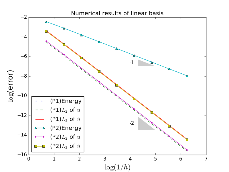
From the error estimates, regardless of whether we use the displacement or velocity form of the internal variables, for this smooth solution we can expect that $\left\lVert e_{h}^{N}\right\rVert_{V}$ , $\left\lVert\tilde{e}_{h}^{N}\right\rVert_{L_{2}(\Omega)}$ , $\left\lVert e_{h}^{N}\right\rVert_{L_{2}(\Omega)}$ , respectively, are of optimal orders $O(h^{s_{1}}+\Delta t^{2})$ , $O(h^{s_{1}+1}+\Delta t^{2})$ , $O(h^{s_{1}+1}+\Delta t^{2})$ respectively (because $s_{2}=\infty$ ). In other words, the convergence rate with respect to time is fixed at second order but the spatial convergence order depends on the degree of polynomials $s_{1}$ used in the finite element space $V^{h}$ .

If we take $\Delta t\sim h$ then we will expect for our errors that

\left\lVert e_{h}^{N}\right\rVert_{V}=O(h^{\min(s_{1},2)}),\qquad\left\lVert\tilde{e}_{h}^{N}\right\rVert_{L_{2}(\Omega)},\left\lVert e_{h}^{N}\right\rVert_{L_{2}(\Omega)}=O(h^{\min(s_{1}+1,2)}).

In the computational results that follow, the numerical convergence rate, $d_{c}$ , is estimated by

d_{c}\ =\ \frac{\log(\text{error of }h_{1})-\log(\text{error of }h_{2})}{\log(h_{1})-\log(h_{2})}.

We can see this in Figure 1 where on the left we give results for a piecewise linear basis ( $s_{1}=1$ ) and on the right hand for a quadratic basis ( $s_{1}=2$ ). The convergence rate is given by the gradients of the lines. With linears the energy errors have first order accuracy but the $L_{2}$ errors show optimal second order. On the other hand, for quadratics, we can observe second order rates for all quantities because the time-error convergence order is fixed at $2$ .

Refer to caption — Figure 1: Numerical convergent order: linear (left) and quadratic (right) polynomial basis

To see the higher order spatial convergence for the quadratic case we take a much smaller $\Delta t$ so that we can consider the time error to be negligible in that,

\left\lVert e_{h}^{N}\right\rVert_{V}\approx O(h^{2})\textrm{ and }\left\lVert\tilde{e}_{h}^{N}\right\rVert_{L_{2}(\Omega)},\left\lVert e_{h}^{N}\right\rVert_{L_{2}(\Omega)}\approx O(h^{3}).

The results are shown in Table 1. In the same way, if we make the spatial error negligible, we can observe the temporal error convergence rate — and this is given in Table 2. We see that the rates are optimal in all cases.

$h$	Displacement form			Velocity form
$h$	$\left\lVert e_{h}^{N}\right\rVert_{V}$	$\left\lVert\tilde{e}_{h}^{N}\right\rVert_{L_{2}(\Omega)}$	$\left\lVert e_{h}^{N}\right\rVert_{L_{2}(\Omega)}$	$\left\lVert e_{h}^{N}\right\rVert_{V}$	$\left\lVert\tilde{e}_{h}^{N}\right\rVert_{L_{2}(\Omega)}$	$\left\lVert e_{h}^{N}\right\rVert_{L_{2}(\Omega)}$
1/4	2.2557E-3	8.1101E-5	6.9417E-5	2.2557E-3	8.1098E-5	6.9419E-5
1/8	6.0301E-4	1.0491E-5	9.2260E-6	6.0301E-4	1.0489E-5	9.2266E-6
1/16	1.5566E-4	1.2803E-6	1.1954E-6	1.5566E-4	1.2794E-6	1.1957E-6
1/32	3.9526E-5	1.6460E-7	1.5240E-7	3.9526E-5	1.6270E-7	1.5226E-7
rate	1.93	2.99	2.93	1.93	2.99	2.93

Table 1: Fixed time step size errors when

s_{1}=2

and

\Delta t=1/1200

$\Delta t$	Displacement form			Velocity form
$\Delta t$	$\left\lVert e_{h}^{N}\right\rVert_{V}$	$\left\lVert\tilde{e}_{h}^{N}\right\rVert_{L_{2}(\Omega)}$	$\left\lVert e_{h}^{N}\right\rVert_{L_{2}(\Omega)}$	$\left\lVert e_{h}^{N}\right\rVert_{V}$	$\left\lVert\tilde{e}_{h}^{N}\right\rVert_{L_{2}(\Omega)}$	$\left\lVert e_{h}^{N}\right\rVert_{L_{2}(\Omega)}$
1/8	6.0705E-04	8.5271E-04	2.4904E-04	3.6453E-04	6.8608E-04	1.4780E-04
1/16	1.5316E-04	2.1327E-04	6.3192E-05	9.2174E-05	1.7163E-04	3.7643E-05
1/32	3.8373E-05	5.3325E-05	1.5856E-05	2.3105E-05	4.2915E-05	9.4542E-06
1/64	9.5993E-06	1.3332E-05	3.9677E-06	5.7818E-06	1.0729E-05	2.3663E-06
rate	1.99	2.00	1.99	1.99	2.00	1.98

Table 2: Fixed spatial mesh size errors when

s_{1}=2

and

h=1/512

In summary, both the displacement form and the velocity form display numerical results consistent with the given error bounds. This is true for the $L_{2}(\Omega)$ estimates even though the elliptic regularity estimate (3.9) is usually only relied upon for homogeneous Dirichlet problems. We included a Neumann boundary condition here for generality but the code could easily be altered to the pure Dirichlet case to conform to the standard requirements for elliptic regularity, although we note that in [29, Chapter 4.3] and [30] there are discussions of elliptic regularity for problems where both Dirichlet and Neumann boundary conditions are present. In any event, our intention was simply to demonstrate that the optimal rates are in fact achieved in practice.

6 Conclusions

Our two fully discrete formulations demonstrate optimal energy and $L_{2}$ spatial error estimates, and second order temporal error estimates, both in theory, and in numerical tests. We took the usual step in assuming ideal conditions for the proofs although in practical problems one cannot always expect such optimality. For example, if we had lower spatial regularity due, say, to corner singularities we would expect the energy estimates to be of the order $O(h^{\min(s_{1}+1,s_{2})-1}+\Delta t^{2})$ where the specific values of the exponents would depend on the geometry and strength of the singularity. Also, with such reduced regularity we would be unlikely to have the necessary elliptic regularity for a higher order $L_{2}$ estimate.

If, on the other hand, the regularity in time was reduced then we would expect to see $\Delta t^{2}$ replaced by $\Delta t^{\beta}$ , for $\beta<2$ , in the above. This may stem from the loads $f$ and $g$ being non-smooth in time, possibly even discontinuous in some applications (we can think of intermittent hammer blows on a structure for example). Our assumptions on the temporal behaviour of $f$ and $g$ are quite strong, and these allowed us to circumvent the use of Grönwall’s lemma. Although it would be an interesting to see how these assumptions could be relaxed while retaining the sharper bounds, we have no choice here but to defer this to a later study.

This scalar, or antiplane shear, problem studied above can can be straighforwardly elevated to a vector-valued problem representing dynamic linear viscoelasticity by making some notational changes and using product Hilbert spaces. For details see, for example, [3, 20] but, in brief, for this we would define the Cauchy infinitesimal strain tensor ${{\varepsilon}}_{ij}(\boldsymbol{u})=\frac{1}{2}\left(\frac{\partial u_{i}}{\partial x_{j}}+\frac{\partial u_{j}}{\partial x_{i}}\right)$ for $i,j=1,\ldots,d$ , $d=2$ or $3$ and where $\boldsymbol{u}$ is the displacement vector. The tensor $\mathchoice{\hbox to0.0pt{{$\underline{{\hbox to3.73055pt{}}}$\hss}}}{\hbox to0.0pt{{$\underline{{\hbox to3.73055pt{}}}$\hss}}}{\hbox to0.0pt{{$\underline{{\hbox to3.0225pt{}}}$\hss}}}{\hbox to0.0pt{{$\underline{{\hbox to2.69862pt{}}}$\hss}}}\boldsymbol{\varepsilon}(\boldsymbol{u})$ then plays the role of $\nabla u$ . We then replace $D$ with $\mathchoice{\hbox to0.0pt{{$\underline{{\hbox to7.76053pt{}}}$\hss}}}{\hbox to0.0pt{{$\underline{{\hbox to7.76053pt{}}}$\hss}}}{\hbox to0.0pt{{$\underline{{\hbox to5.43236pt{}}}$\hss}}}{\hbox to0.0pt{{$\underline{{\hbox to3.88025pt{}}}$\hss}}}\boldsymbol{D}$ , a symmetric positive definite fourth order tensor, and the stress tensor $\mathchoice{\hbox to0.0pt{{$\underline{{\hbox to4.5713pt{}}}$\hss}}}{\hbox to0.0pt{{$\underline{{\hbox to4.5713pt{}}}$\hss}}}{\hbox to0.0pt{{$\underline{{\hbox to3.70715pt{}}}$\hss}}}{\hbox to0.0pt{{$\underline{{\hbox to3.26068pt{}}}$\hss}}}\boldsymbol{\sigma}$ is given in direct analogy to the scalar analogues in (1.6) and (1.7). The resulting variational formulation uses the symmetric bilinear form $a(\boldsymbol{w},\boldsymbol{v})=\left(\mathchoice{\hbox to0.0pt{{$\underline{{\hbox to7.76053pt{}}}$\hss}}}{\hbox to0.0pt{{$\underline{{\hbox to7.76053pt{}}}$\hss}}}{\hbox to0.0pt{{$\underline{{\hbox to5.43236pt{}}}$\hss}}}{\hbox to0.0pt{{$\underline{{\hbox to3.88025pt{}}}$\hss}}}\boldsymbol{D}\mathchoice{\hbox to0.0pt{{$\underline{{\hbox to3.73055pt{}}}$\hss}}}{\hbox to0.0pt{{$\underline{{\hbox to3.73055pt{}}}$\hss}}}{\hbox to0.0pt{{$\underline{{\hbox to3.0225pt{}}}$\hss}}}{\hbox to0.0pt{{$\underline{{\hbox to2.69862pt{}}}$\hss}}}\boldsymbol{\varepsilon}(\boldsymbol{w}),\mathchoice{\hbox to0.0pt{{$\underline{{\hbox to3.73055pt{}}}$\hss}}}{\hbox to0.0pt{{$\underline{{\hbox to3.73055pt{}}}$\hss}}}{\hbox to0.0pt{{$\underline{{\hbox to3.0225pt{}}}$\hss}}}{\hbox to0.0pt{{$\underline{{\hbox to2.69862pt{}}}$\hss}}}\boldsymbol{\varepsilon}(\boldsymbol{v})\right)$ for $\boldsymbol{w},\boldsymbol{v}\in\boldsymbol{V}$ where $\boldsymbol{V}=\{\boldsymbol{v}\in[H^{1}(\Omega)]^{d}\ |\ \boldsymbol{v}(\boldsymbol{x})=0\textrm{ on }\Gamma_{D}\}$ . The coercivity of this form follows from Korn’s inequality (e.g. [31, 32, 33, 27]), and continuity follows from the Cauchy-Schwarz inequality. Internal variables can be defined by exact analogy with those above, and continous and discrete variational problems can similarly posed. The stability and error analyses then go through in the same way as above with the help of the elasticity theory estimates in [34, 27, 35], and we will obtain similarly optimal bounds without the use of Grönwall’s inequality.

References

[1] S. C. Hunter, Mechanics of continuous media, Halsted Press, 1976 (1976).
[2] S. Shaw, J. R. Whiteman, Some partial differential Volterra equation problems arising in viscoelasticity, in: Proceedings of Equadiff, Vol. 9, 1998, pp. 183–200 (1998).
[3] B. Rivière, S. Shaw, J. R. Whiteman, Discontinuous Galerkin finite element methods for dynamic linear solid viscoelasticity problems, Numerical Methods for Partial Differential Equations 23 (5) (2007) 1149–1166 (2007).
[4] J. Barber, Elasticity, Springer Netherlands, Dordrecht, 2004 (2004). doi:10.1007/0-306-48395-5\_15.
URL https://doi.org/10.1007/0-306-48395-5-15
[5] G. Paulino, Z.-H. Jin, Viscoelastic functionally graded materials subjected to antiplane shear fracture, Journal of applied mechanics 68 (2) (2001) 284–293 (2001).
[6] T.-V. Hoarau-Mantel, A. Matei, Analysis of a viscoelastic antiplane contact problem with slip-dependent friction, Applied Mathematics and Computer Science 12 (1) (2002) 51–58 (2002).
[7] W. N. Findley, F. A. Davis, Creep and relaxation of nonlinear viscoelastic materials, Courier Corporation, 2013 (2013).
[8] J. M. Golden, G. A. Graham, Boundary value problems in linear viscoelasticity, Springer Science & Business Media, 2013 (2013).
[9] A. R. Johnson, Modeling viscoelastic materials using internal variables, in: The Shock and Vibration Digest, Vol. 31, 1999, pp. 91–100 (03 1999).
[10] T. H. Grönwall, Note on the derivatives with respect to a parameter of the solutions of a system of differential equations, Annals of Mathematics (1919) 292–296 (1919).
[11] J. M. Holte, Discrete Grönwall lemma and applications, in: MAA-NCS meeting at the University of North Dakota, Vol. 24, 2009, pp. 1–7 (2009).
[12] B. Rivière, Discontinuous Galerkin methods for solving elliptic and parabolic equations: theory and implementation, SIAM, 2008 (2008).
[13] V. Thomée, Galerkin finite element methods for parabolic problems, Vol. 1054, Springer, 1984 (1984).
[14] M. Alnæs, J. Blechta, J. Hake, A. Johansson, B. Kehlet, A. Logg, C. Richardson, J. Ring, M. E. Rognes, G. N. Wells, The fenics project version 1.5, Archive of Numerical Software 3 (100) (2015) 9–23 (2015).
[15] Y. Jang, Spatially continuous and discontinuous Galerkin finite element approximations for dynamic viscoelastic problems, Ph.D. thesis, Brunel University London, http://bura.brunel.ac.uk/handle/2438/21084 (2020).
[16] S. Shaw, M. K. Warby, J. R. Whiteman, Error estimates with sharp constants for a fading memory Volterra problem in linear solid viscoelasticity, SIAM J. Numer. Anal. 34 (1997) 1237—1254 (1997).
[17] S. Shaw, J. R. Whiteman, Optimal long-time ${L}_{p}(0,{T})$ data stability and semidiscrete error estimates for the Volterra formulation of the linear quasistatic viscoelasticity problem, Numer. Math. 88 (2001) 743—770, (BICOM Tech. Rep. 98/7 see: www.brunel.ac.uk/bicom) (2001).
[18] B. Rivière, S. Shaw, M. F. Wheeler, J. R. Whiteman, Discontinuous Galerkin finite element methods for linear elasticity and quasistatic linear viscoelasticity, Numer. Math. 95 (2003) 347—376 (2003).
[19] S. Shaw, J. R. Whiteman, A posteriori error estimates for space-time finite element approximation of quasistatic hereditary linear viscoelasticity problems, Comput. Methods Appl. Mech. Engrg. 193 (2004) 5551—5572, (See also Technical Report 03/2 at www.brunel.ac.uk/bicom) (2004).
[20] S. Shaw, An a priori error estimate for a temporally discontinuous Galerkin space-time finite element method for linear elasto- and visco-dynamics, Comput. Meth. Appl. Mech. Eng. 351 (2019) 1—19 (2019).
[21] S. Shaw, J. R. Whiteman, Numerical solution of linear quasistatic hereditary viscoelasticity problems, SIAM J. Numer. Anal 38 (1) (2000) 80—97 (2000).
[22] E. G. Yanik, G. Fairweather, Finite element methods for parabolic and hyperbolic partial integro-differential equations, Nonlinear Analysis, Theory, Methods & Applications 12 (1988) 785—809 (1988).
[23] A. K. Pani, V. Thomée, L. B. Wahlbin, Numerical methods for hyperbolic and parabolic integro-differential equations, J. Integral Equations Appl. 4 (1992) 533—584 (1992).
[24] C. M. Dafermos, An abstract Volterra equation with applications to linear viscoelasticity, J. Diff. Eqns. 7 (1970) 554—569 (1970).
[25] C. Gräser, A note on Poincaré- and Friedrichs-type inequalities, arXiv preprint arXiv:1512.02842 (2015).
[26] M. F. Wheeler, A priori ${L}_{2}$ error estimates for Galerkin approximations to parabolic partial differential equations, SIAM Journal on Numerical Analysis 10 (4) (1973) 723–759 (1973).
[27] S. Brenner, R. Scott, The mathematical theory of finite element methods, Vol. 15, Springer Science & Business Media, 2007 (2007).
[28] M. Dauge, Elliptic boundary value problems on corner domains, volume 1341 of Lecture Notes in Mathematics, Springer-Verlag, Berlin, 1988 (1988).
[29] P. Grisvard, Elliptic problems in nonsmooth domains, SIAM, 2011 (2011).
[30] M. Costabel, M. Dauge, S. Nicaise, Analytic regularity for linear elliptic systems in polygons and polyhedra, Mathematical Models and Methods in Applied Sciences 22 (8) (2012) 1250015–1 — 1250015–63, doi 10.1142/S0218202512500157, hal-00454133v3 (2012).
[31] P. G. Ciarlet, On Korn’s inequality, Chinese Annals of Mathematics, Series B 31 (5) (2010) 607–618 (2010).
[32] C. O. Horgan, L. E. Payne, On inequalities of Korn, Friedrichs and Babuška-Aziz, Archive for Rational Mechanics and Analysis 82 (2) (1983) 165–179 (1983).
[33] J. A. Nitsche, On Korn’s second inequality, RAIRO. Analyse numérique 15 (3) (1981) 237–248 (1981).
[34] S. C. Brenner, L.-Y. Sung, Linear finite element methods for planar linear elasticity, Mathematics of Computation 59 (200) (1992) 321–338 (1992).
[35] M. Amara, J.-M. Thomas, Equilibrium finite elements for the linear elastic problem, Numerische Mathematik 33 (4) (1979) 367–383 (1979).