跳到论文正文
W Papers独立论文阅读器 arXiv:2001.04578 论文正文 计算阅读时间 · 0%
引用这篇论文根据当前论文元数据生成,正式投稿前建议核对。


License: arXiv.org perpetual non-exclusive license
arXiv:2001.04578v2 [math.DG] 28 Feb 2021

Generalizations of the theorems of Pappus-Guldin in the Heisenberg groupsVolume: Volume , Number 0,

Yen-Chang Huang Address: Yen-Chang Huang
Department of Applied Mathematics
National University of Tainan
Tainan, Taiwan
Email address: ychuang@mail.nutn.edu.tw
© , Korean Mathematical Society
Abstract.

In this paper we study areas (called p-areas) and volumes for parametric surfaces in the 3D-Heisenberg group ℍ1\mathbb{H}_{1}, which is considered as a flat model of pseudo-hermitian manifolds. We derive the formulas of p-areas and volumes for parametric surfaces in ℍ1\mathbb{H}_{1} and show that the classical result of Pappus-Guldin theorems for surface areas and volumes hold if the surfaces satisfy some geometric properties. Some examples are also provided, including the surfaces with constant p-mean curvatures.

Key words and phrases: 
Pappus-Guldin Theorem, Sub-Riemannian manifolds, Pseudo-hermitian geometry
2010 Mathematics Subject Classification
Primary: 53C17, Secondary: 53C65, 53C23

1. Introduction

A remarkable formula for the volumes and surface areas of solid objects in ℝ3\mathbb{R}^{3} was given by A. Pappus about AD 300 and was rediscovered by P. Guldin in 1641 in many Calculus books. Nowadays the theorem is known as Pappus-Guldin theorem or Pappus theorem. We refer the interested readers to [15, 17] about a short historical review of the development of the theorem, including the early generalizations by Euler and Richter. The papers [3] and [19] mentioned the reasons why mathematicians in the 17th century did not know the work of Pappus.

The Pappus-Guldin theorem states the method of finding volumes and surface areas respectively for any solid of revolution into two parts:

Theorem A.

The volume of a solid of revolution MM generated by rotating a region ℛ\mathcal{R} about a line ℓ\ell that does not meet ℛ\mathcal{R} is given by

V​o​l​u​m​e​(M)=A​r​e​a​(ℛ)×s0,Volume(M)=Area(\mathcal{R})\times s_{0},

where s0s_{0} is the perimeter of the circle described by the centroid of ℛ\mathcal{R} during the rotation.

Theorem B.

The surface area of a surface of revolution Σ\Sigma generated by rotating a plane curve 𝒞0\mathcal{C}_{0} about an axis ℓ\ell that does not meet 𝒞0\mathcal{C}_{0} is given by

A​r​e​a​(Σ)=L​e​n​g​t​h​(𝒞0)×s0,Area(\Sigma)=Length(\mathcal{C}_{0})\times s_{0},

where s0s_{0} is the length of the curve described by the centroid of 𝒞0\mathcal{C}^{0} during the rotation.

In [15] A.W. Goodman and G. Goodman gave a proof of the generalization of Theorem A for domain MM generated by moving a plane region ℛ\mathcal{R} around an arbitrary space curve γ\gamma. When the center of mass of ℛ\mathcal{R} is on γ\gamma, they have

V​o​l​u​m​e​(M)=A​r​e​a​(ℛ)×L​e​n​g​t​h​(γ).Volume(M)=Area(\mathcal{R})\times Length(\gamma).

However, the authors showed that Theorem B holds only for the surface area of Σ\Sigma generated by moving a plane curve 𝒞0\mathcal{C}_{0} around a plane curve γ\gamma with ”natural motions” (see [15, p358]). After that, Flanders [13] and Pursell [18] supplemented the results of surface areas in [15] by showing that there exists a unique spin function such that the area of the surface Σ\Sigma generated by 𝒞0\mathcal{C}_{0}, when 𝒞0\mathcal{C}_{0} moves with the spin, agrees with the result of Theorem B

A​r​e​a​(Σ)=L​e​n​g​t​h​(𝒞0)×L​e​n​g​t​h​(γ).Area(\Sigma)=Length(\mathcal{C}_{0})\times Length(\gamma).

On one hand, Pursell used the classical method of differential geometry and showed that the ”natural motion” in [15] is actually a motion with 𝒞0\mathcal{C}_{0} fixed to a Frenet frame. On the other hand, Flanders obtained the result of Theorem B in a more efficient method by using moving frames and differential forms. In addition, Gray-Miquel [16] also generalized Pappus-type theorems for volumes and surface areas to the hypersurfaces in the space forms. We also stress that there is a natural connection between Pappus-Guldin formula and the works by H. Weyl. In [25] Weyl proved the formulas of the volumes of a tube PrP_{r} with radius rr and the corresponding tubular hypersurface ∂Pr\partial P_{r} around a qq-dimensional submanifold PP in a Euclidean or Spherical space, and finally those formulas were used later in the proof of the generalized Gauss-Bonnet Theorem by Allendoerfer [1] and Fenchel [12]. We refer the reader to the book [25] and the survey [24] by Vanhecke for more details about the connection of Weyl’s works and Pappus-Guldin theorem.

In the last years the study of variational problems in sub-Riemannian geometry and pseudo-hermitian geometry have received an increasing interest. Especially the desire to achieve a better understanding of questions of global geometry involving the areas and volumes, such as the Plateau problem or the isoperimetric problem, has motivated the recent development of a theory of Pappus-Guldin theorem. More precisely, in the present paper we ask the following questions:

Does Pappus-Guldin theorem hold in the Heisenberg group ℍ1\mathbb{H}_{1}? What are the appropriate geometric quantities (lengths, surface areas, volumes) satisfying the geometry of ℍ1\mathbb{H}_{1} as a standard model of sub-Riemannian manifolds?

The answer is affirmative if we take the following geometric quantities: (1) horizontal lengths for curves, (2) p-area for surface areas (defined in next section), (3) Euclidean volumes for solid domain in ℍ1\mathbb{H}_{1}. We shall show the generalization of Pappus-Guldin theorem for volumes and surface areas of any tube consisting of a plane region moving along a curve passing through the region.

In [15, p 385] the authors considered the tubes in ℝ3\mathbb{R}^{3} constructed by the following method: given a C3C^{3}-closed curve

R​(s)=(x⁡(s),y⁡(s),z⁡(s))\textbf{R}(s)=\big(x(s),y(s),z(s)\big)

for s∈[0,s0]s\in[0,s_{0}] and a Frenet frame {T​(s),N​(s),B​(s)}\{\textbf{T}(s),\textbf{N}(s),\textbf{B}(s)\} defined on R​(s)\textbf{R}(s), where the unit vectors T,N,B\textbf{T},\textbf{N},\textbf{B} are the tangent, the normal, and the binormal vectors, respectively. By setting x⁡(0)>0x(0)>0, y⁡(0)=z⁡(0)=0y(0)=z(0)=0, and the initial point R​(0)=(x⁡(0),y⁡(0),z⁡(0))=(x⁡(s0),y⁡(s0),z⁡(s0))∈R​(s)\textbf{R}(0)=\big(x(0),y(0),z(0)\big)=\big(x(s_{0}),y(s_{0}),z(s_{0})\big)\in\textbf{R}(s), the authors also defined the plane curve by

𝒞0:R1​(t)=(f⁡(t),g⁡(t),0),\mathcal{C}_{0}:\textbf{R}_{1}(t)=\big(f(t),g(t),0\big),

for some C1C^{1}-functions f⁡(t),g⁡(t)f(t),g(t) defined on [0,t0][0,t_{0}]. Note that the point R​(0)\textbf{R}(0) is regarded as the origin for describing the curve 𝒞0\mathcal{C}_{0}. Thus, the plane region ℛ∋R​(0)\mathcal{R}\ni\textbf{R}(0) enclosed by 𝒞0\mathcal{C}_{0} lies on the x​yxy-plane (as shown in Fig. 1). The ”natural motion” of the region ℛ\mathcal{R} along the curve R​(s)\textbf{R}(s) is defined by choosing the coordinate system so that at s=0s=0, the vectors T and N lie on the x​zxz-plane, and N lies on the xx-axis pointed toward the origin. When the region ℛ\mathcal{R} moves along R​(s)\textbf{R}(s) starting from R​(0)\textbf{R}(0), ℛ\mathcal{R} is always on the plane spanned by N​(s)\textbf{N}(s) and B​(s)\textbf{B}(s), and the line segment contained in B​(0)\textbf{B}(0) at R​(0)\textbf{R}(0) is always contained in B​(s)\textbf{B}(s) for any ss. More precisely, the surface Σ\Sigma generated by moving the plane region ℛ\mathcal{R} along the curve R​(s)\textbf{R}(s) can be represented by the parametrized surface

(1) 𝕏⁡(s,t)=R​(s)−f⁡(t)​N​(s)−g⁡(t)​B​(s),\displaystyle\mathbb{X}(s,t)=\textbf{R}(s)-f(t)\textbf{N}(s)-g(t)\textbf{B}(s),

Note that when the region ℛ\mathcal{R} moves along the curve R​(s)\textbf{R}(s), ℛ\mathcal{R} is always perpendicular to the tangent vector T.

Refer to caption
Figure 1. ”Natural motion” of the region ℛ\mathcal{R} along the closed curve R(s)

Next we begin to set up for this case. Regarding 3-dimensional Heisenberg group ℍ1\mathbb{H}_{1} as the standard model of the pseudo-hermitian manifolds, there exists the contact planes ξp\xi_{p} and the CR structure JJ defined for all point p∈ℍ1p\in\mathbb{H}_{1}. For some fundamental background about ℍ1\mathbb{H}_{1}, we refer the readers to the next section. Unlike the surfaces in [15] that the authors only consider the surfaces generated by the vectors N and B in (1), in the 3-dimensional Heisenberg group ℍ1\mathbb{H}_{1} we consider a more generalized surface

(2) Σ:𝕏⁡(s,t)=γ⁡(s)+f⁡(t)​U​(s)+g⁡(t)​V​(s)+h⁡(t)​T,\displaystyle\Sigma:\mathbb{X}(s,t)=\gamma(s)+f(t)U(s)+g(t)V(s)+h(t)T,

for some real-valued functions f⁡(t),g⁡(t),h⁡(t)f(t),g(t),h(t) with suitable regularity. Here γ⁡(s)\gamma(s) is a horizontally regular curve with horizontal arc-length, i.e., the orthogonal decomposition of the velocity vector γ′​(s)=γξ′​(s)+γT′​(s)\gamma^{\prime}(s)=\gamma^{\prime}_{\xi}(s)+\gamma^{\prime}_{T}(s) has the nonzero contact part γξ′​(s)∈ξγ⁡(s)\gamma^{\prime}_{\xi}(s)\in\xi_{\gamma(s)} and |γξ′|=1|\gamma^{\prime}_{\xi}|=1 w.r.t. the Levi-metric ⟨X,Y⟩=12​d​Θ​(X,J​Y)\langle X,Y\rangle=\frac{1}{2}d\Theta(X,JY) for any vectors X,YX,Y in ℍ1\mathbb{H}_{1}, and U⁡(s)=γξ​(s),V⁡(s)=J​γξ​(s)U(s)=\gamma_{\xi}(s),V(s)=J\gamma_{\xi}(s), T=∂∂zT=\frac{\partial}{\partial z}, and JJ is the CR structure. Note that {U⁡(s),V⁡(s),T}\{U(s),V(s),T\} forms an orthonormal basis w.r.t. the Levi-metric. A more natural perspective for the setting of (2) is that when considering ℍ1\mathbb{H}_{1} as the Lie group with the group operation defined by (10) (see next section), the surface Σ\Sigma can be obtained by moving the frame {U⁡(0),V⁡(0),T}\{U(0),V(0),T\} at the origin along the curve γ⁡(s)\gamma(s). More precisely, the parametrization of (2) can be equivalently defined by

(2’) Σ:𝕏⁡(s,t)=Lγ⁡(s)​(f⁡(t)​U​(0)+g⁡(t)​V​(0)+h⁡(t)​T),\displaystyle\Sigma:\mathbb{X}(s,t)=L_{\gamma(s)}\big(f(t)U(0)+g(t)V(0)+h(t)T\big),

where U⁡(0)U(0) and V⁡(0)V(0) are two fixed unit vectors starting from the origin and ending at somewhere on the x​yxy-plane. Indeed, suppose γ⁡(0)=0∈ℍ1\gamma(0)=0\in\mathbb{H}_{1} and since |γξ′​(s)|=1|\gamma^{\prime}_{\xi}(s)|=1, we may set U⁡(s)=η​e̊1​(γ⁡(s))+ζ​e̊2​(γ⁡(s))U(s)=\eta\mathring{e}_{1}(\gamma(s))+\zeta\mathring{e}_{2}(\gamma(s)) and V⁡(s)=−ζ​e̊1​(γ⁡(s))+η​e̊2​(γ⁡(s))V(s)=-\zeta\mathring{e}_{1}(\gamma(s))+\eta\mathring{e}_{2}(\gamma(s)) for some real numbers with η2+ζ2=1\eta^{2}+\zeta^{2}=1. Here e̊1,e̊2\mathring{e}_{1},\mathring{e}_{2} are the standard basis of the invariant vector fields defined by (11). In particular, U⁡(0)=(η,ζ,0)U(0)=(\eta,\zeta,0) and V⁡(0)=(−ζ,η,0)V(0)=(-\zeta,\eta,0). By using the group operation (10) one has

Lγ⁡(s)​(f​(t)​U​(0)CLOSE\displaystyle L_{\gamma(s)}\big(f(t)U(0) OPEN+g⁡(t)​V​(0)+h⁡(t)​T)\displaystyle+g(t)V(0)+h(t)T\big)
=(x⁡(s),y⁡(s),z⁡(s))⋅(f⁡(t)​η−g⁡(t)​ζ,f⁡(t)​ζ+g⁡(t)​η,h⁡(t))\displaystyle=\big(x(s),y(s),z(s)\big)\cdot\big(f(t)\eta-g(t)\zeta,f(t)\zeta+g(t)\eta,h(t)\big)
=γ⁡(s)+f⁡(t)​[η​e̊1​(γ⁡(s))+ζ​e̊2​(γ⁡(s))]+g⁡(t)​[−ζ​e̊1​(γ⁡(s))+η​e̊2​(γ⁡(s))]+h⁡(t)​T\displaystyle=\gamma(s)+f(t)\Big[\eta\mathring{e}_{1}(\gamma(s))+\zeta\mathring{e}_{2}(\gamma(s))\Big]+g(t)\Big[-\zeta\mathring{e}_{1}(\gamma(s))+\eta\mathring{e}_{2}(\gamma(s))\Big]+h(t)T
=γ⁡(s)+f⁡(t)​U​(s)+g⁡(t)​V​(s)+h⁡(t)​T,\displaystyle=\gamma(s)+f(t)U(s)+g(t)V(s)+h(t)T,

and so (2) and (2’) are equivalent.

Analogous to the settings in [15], the surface of revolution Σ\Sigma is defined by rotating the closed space curve

𝒞s​(t):f⁡(t)​U​(s)+g⁡(t)​V​(s)+h⁡(t)​T\mathcal{C}_{s}(t):f(t)U(s)+g(t)V(s)+h(t)T

for some fixed s∈[0,s0]s\in[0,s_{0}] along the closed curve

γ⁡(s)=(x⁡(s),y⁡(s),z⁡(s)).\gamma(s)=\big(x(s),y(s),z(s)\big).

Throughout this paper we always use the parameter s∈[0,s0]s\in[0,s_{0}] for the curve γ\gamma and the frames U,VU,V along γ\gamma, and use the parameter t∈[0,t0]t\in[0,t_{0}] for the functions f,g,h,f,g,h, describing the curve 𝒞s\mathcal{C}_{s}. For simplicity, we shall also drop out the parameters in derivatives if the notion is clear, for instance, f′​U+g​V′f^{\prime}U+gV^{\prime} means d​f​(t)d​t​U​(s)+g⁡(t)​d​V​(s)d​s\frac{df(t)}{dt}U(s)+g(t)\frac{dV(s)}{ds}. We often denote MM by the solid of revolution and ∂M\partial M or Σ\Sigma by its surface. Also, in the present paper we only consider the surface 𝕏⁡(s,t)\mathbb{X}(s,t) defined by (2) satisfying these fundamental assumptions:

  1. (A1)

    The closed curve 𝒞s​(t)\mathcal{C}_{s}(t) does not intersect itself when moving along the curve γ⁡(s)\gamma(s).

  2. (A2)

    The domain enclosed by the parametrized surface Σ\Sigma defined by (2) is not self-intersected.

For the regularity of the functions γ\gamma, and f,g,hf,g,h, we have the minimal assumptions for the order of derivatives necessary to carry out the proofs. It turns out that the requirements are different for the two curves γ\gamma and 𝒞s\mathcal{C}_{s}. For γ⁡(s)\gamma(s) we require that the third derivatives γ′′′\gamma^{{}^{\prime\prime\prime}} be continuous in the interval 0≤s≤s00\leq s\leq s_{0}. We emphasis that γ\gamma may not necessarily be closed, but if it is closed we have to assume that γ(k)​(0)=γ(k)​(s0)\gamma^{(k)}(0)=\gamma^{(k)}(s_{0}) for k=0,1,2,3,k=0,1,2,3, where γ(k)\gamma^{(k)} is the kk-th derivative with respect to the horizontal arc-length ss. For the closed curve 𝒞s\mathcal{C}_{s} (when fixed ss), in the first glance, it seems that we need to have the functions f⁡(t),g⁡(t),h⁡(t)f(t),g(t),h(t) be C1C^{1}-functions in the interval 0≤t≤t00\leq t\leq t_{0}, except for Corollary 5.5 that we need a C2C^{2}-assumption for those functions. However, a stronger regularity assumption is needed to avoid the issue of singular points. A point on a surface in ℍ1\mathbb{H}_{1} is called singular if the contact plane and tangent plane at that point coincide with each other; otherwise, it is called regular (see next section for more detail). According to [6, Theorem 3.3 or Theorem B], a singular point on a C2C^{2}-smooth surface is either isolated or passed through by a C1C^{1}-smooth singular curve in a neighborhood if the p-mean curvature is bounded. Since the p-mean curvature needs C2C^{2}-regularity for the surface, throughout the whole paper we always assume that the functions f⁡(t),g⁡(t),h⁡(t)f(t),g(t),h(t) are of C2C^{2}-regularity. Thus, the set of singular points on the constructed surfaces has measure zero with respect to the area and volume measures and so we can ignore the influence of the singular point when considering the surface areas and volumes.

Next we introduce the appropriate geometric quantities for Pappus-Guldin Theorem. Let MM be a domain with boundary ∂M\partial M in ℍ1\mathbb{H}_{1}. For any point p∈∂Mp\in\partial M is not a singular point, denote by the unit vector e1​(p)=T​Mp∩ξpe_{1}(p)=TM_{p}\cap\xi_{p}, e2=J​e1e_{2}=Je_{1}, and the standard contact form Θ=d​z+x​d​y−y​d​x\Theta=dz+xdy-ydx, where JJ is the CR structure, J2=−1J^{2}=-1. The set {e1,e2,T}\{e_{1},e_{2},T\} forms an standard orthonormal frame with the corresponding coframe {e1,e2,Θ}\{e^{1},e^{2},\Theta\}. As we know that the appropriate notions for volumes and areas in ℍ1\mathbb{H}_{1} are the Euclidean volumes and the p-areas, respectively, and the p-area can be obtained by the variation of the volume form along the e2e_{2}-direction (equation (2.5) in [6, p135]). More precisely, those geometric quantities are defined by

(3) V​o​l​u​m​e​(M)\displaystyle Volume(M) :=V⁡(M)=12​∫MΘ∧𝑑Θ,\displaystyle:=V(M)=\frac{1}{2}\int_{M}\Theta\wedge d\Theta,
p​-​a​r​e​a​(∂M)\displaystyle p\text{-}area(\partial M) :=𝒜⁡(M)=∫∂MΘ∧e1,\displaystyle:=\mathcal{A}(M)=\int_{\partial M}\Theta\wedge e^{1},

where Θ∧e1\Theta\wedge e^{1} is called the p-area form. Note that the volumes and the p-areas are invariant under the ”rigid motions” in ℍ1\mathbb{H}_{1}, namely, they are invariant under the group of pseudo-Hermitian transformations in ℍ1\mathbb{H}_{1}, P​H​S​(1)PHS(1), which consists of the left translations and the elements in the unitary group U⁡(1)U(1). For the details of this group P​S​H​(n)PSH(n), we refer the reader to [9] for n=1n=1 and [10] for n≥1n\geq 1; both papers are the first published papers studying on the fundamental theorems for curves and hypersurfaces in the Heisenberg groups.

A key observation for the study of Pappus-Guldin theorem is shown in Proposition 3.2: for any parametric surface Σ:𝕏⁡(s,t)=(X⁡(s,t),Y⁡(s,t),Z⁡(s,t))\Sigma:\mathbb{X}(s,t)=\big(X(s,t),Y(s,t),Z(s,t)\big) in ℍ1\mathbb{H}_{1} we derive the p-area form d​Σpd\Sigma_{p} at the nonsingular point p∈Σp\in\Sigma, namely,

(4) d​Σp=A2+B2​d​s​d​t,\displaystyle d\Sigma_{p}=\sqrt{A^{2}+B^{2}}dsdt,

where

A\displaystyle A :=Zs​Xt−Xs​Zt+X⁡(Xt​Ys−Xs​Yt),\displaystyle:=Z_{s}X_{t}-X_{s}Z_{t}+X(X_{t}Y_{s}-X_{s}Y_{t}),
B\displaystyle B :=Zs​Yt−Ys​Zt+Y⁡(Xt​Ys−Xs​Yt),\displaystyle:=Z_{s}Y_{t}-Y_{s}Z_{t}+Y(X_{t}Y_{s}-X_{s}Y_{t}),

and the subscripts mean the partial derivatives with respect to the specific variables. By using the divergence Theorem (Proposition 3.7), the volume enclosed by the surface Σ\Sigma can be represented by the integral over Σ\Sigma. Moreover, when Σ\Sigma is generated by the curve γ⁡(s)\gamma(s) and the functions f⁡(t),g⁡(t),h⁡(t)f(t),g(t),h(t) as defined by (2), we obtain the first result showing that the volume of an enclosed tube-shaped domain can be obtained by the information from its surface.

Theorem 1.1.

Let MM be a domain in the 3-dimensional Heisenberg group ℍ1\mathbb{H}_{1} with boundary ∂M\partial M, described by the parametrized surface 𝕏⁡(s,t)=γ⁡(s)+f⁡(t)​U​(s)+g⁡(t)​V​(s)+h⁡(s)​T\mathbb{X}(s,t)=\gamma(s)+f(t)U(s)+g(t)V(s)+h(s)T for any (s,t)∈[0,s0]×[0,t0](s,t)\in[0,s_{0}]\times[0,t_{0}], where γ⁡(s)\gamma(s) is a horizontally regular curve (may not be necessarily closed), U⁡(s)=γξ′U(s)=\gamma^{\prime}_{\xi}, and V⁡(s)=J​γξ′V(s)=J\gamma^{\prime}_{\xi}. If MM satisfies the conditions (A​1),(A​2)(A1),(A2), then the volume of MM is given by

(5) V​o​l​u​m​e​(M)\displaystyle Volume(M) =∬κ⁡(x​x′+y​y′)​h′​f+∬(y​x′−y′​x)​κ​h′​g+∬κ​h′​f2−∬τ​g′​f\displaystyle=\iint\kappa(xx^{\prime}+yy^{\prime})h^{\prime}f+\iint(yx^{\prime}-y^{\prime}x)\kappa h^{\prime}g+\iint\kappa h^{\prime}f^{2}-\iint\tau g^{\prime}f
+∬κg2h′+∬(2τ−z′)f′g+s0⋅∫0t0(gg′f−h′g−f′g2)dt,\displaystyle+\iint\kappa g^{2}h^{\prime}+\iint(2\tau-z^{\prime})f^{\prime}g+s_{0}\cdot\int_{0}^{t_{0}}\Big(gg^{\prime}f-h^{\prime}g-f^{\prime}g^{2}\Big)dt,

where all double integrals are taken over the domain [0,s0]×[0,t0][0,s_{0}]\times[0,t_{0}].

Remark 1.2.

Recently Chiu-Ho ([8], Theorem 2.1) defined the Gauss map G:γ→𝕊1⊂ξ0​(0)G:\gamma\rightarrow\mathbb{S}^{1}\subset\xi_{0}(0) by G(p)=Lp−1∗e2G(p)=L_{p^{-1}*}e_{2} for horizontally regular closed cure γ\gamma in ℍ1\mathbb{H}_{1}. They also showed that the degree of the Gauss map satisfying d​e​g​G=12​π​∫0s0κ⁡(s)​𝑑sdegG=\frac{1}{2\pi}\int_{0}^{s_{0}}\kappa(s)ds. Therefore, the third and eighth terms in Theorem 1.1 can be written in terms of the topological information of MM by ∬κ​h′​f2=2​π​𝑑e​g​G​∫0t0h′​f​𝑑t\iint\kappa h^{\prime}f^{2}=2\pi degG\int_{0}^{t_{0}}h^{\prime}fdt and ∬κ​g2​h′=2​π​𝑑e​g​G​∫0t0g2​h′​𝑑t\iint\kappa g^{2}h^{\prime}=2\pi degG\int_{0}^{t_{0}}g^{2}h^{\prime}dt, respectively.

By the definition (13) of the p-curvatures, the assumption κ=0\kappa=0 for the curve γ\gamma is equivalent to that the projection of γ\gamma onto the x​yxy-plane is a line. The following result shows that when κ⁡(s)≡0\kappa(s)\equiv 0 and f⁡(t)≡0f(t)\equiv 0, the volume of the enclosed tube-shaped domain satisfies Pappus-Guldin theorem.

Corollary 1.3 (Pappus-Guldin Theorem for volumes).

Let γ⁡(s)\gamma(s) be a horizontally regular curve parametrized by horizontal arc-length with p-curvature κ⁡(s)≡0\kappa(s)\equiv 0. Suppose the parametrized surface 𝕏⁡(s,t)\mathbb{X}(s,t), given by moving the plane region ℛ\mathcal{R} enclosed by the plane curve 𝒞0​(t)=γ⁡(0)+g⁡(t)​U​(0)+h⁡(t)​T\mathcal{C}_{0}(t)=\gamma(0)+g(t)U(0)+h(t)T along γ\gamma is defined as

𝕏⁡(s,t)=γ⁡(s)+g⁡(t)​U​(s)+h⁡(t)​T\mathbb{X}(s,t)=\gamma(s)+g(t)U(s)+h(t)T

for any (s,t)∈[0,s0]×[0,t0](s,t)\in[0,s_{0}]\times[0,t_{0}] satisfying the assumptions (A​1)(A1), (A​2)(A2). Then the volume of enclosed domain MM by 𝕏⁡(s,t)\mathbb{X}(s,t) satisfies Pappus-Guldin theorem, namely,

V⁡(M)=12⋅horizontal length​(γ)⋅𝒜⁡(ℛ),\displaystyle V(M)=\frac{1}{2}\cdot\text{{horizontal length}}(\gamma)\cdot\mathcal{A}(\mathcal{R}),

where 𝒜⁡(R)\mathcal{A}(R) is the p-area of the area of ℛ\mathcal{R}.

Our second result shows that the p-area form of the parametrized surface Σ\Sigma defined by (2) can be achieved in terms of γ,f,g,h\gamma,f,g,h and their derivatives by substituting the surface into (4).

Theorem 1.4.

Given a horizontally regular curve γ⁡(s)=(x⁡(s),y⁡(s),z⁡(s))\gamma(s)=(x(s),y(s),z(s)) parametrized by the horizontal arc-length ss with the p-curvature κ\kappa and contact normality τ\tau defined by (13), (14) respectively in the Heisenberg group ℍ1\mathbb{H}_{1}. For any C1C^{1}-functions f⁡(t),g⁡(t),h⁡(t)f(t),g(t),h(t), suppose the parametrized surface Σ\Sigma defined by (2)

𝕏:(s,t)∈[0,s0]×[0,t0]↦γ⁡(s)+f⁡(t)​U​(s)+g⁡(t)​V​(s)+h⁡(t)​T,\displaystyle\mathbb{X}:(s,t)\in[0,s_{0}]\times[0,t_{0}]\mapsto\gamma(s)+f(t)U(s)+g(t)V(s)+h(t)T,

satisfying the assumption (A​1),(A​2)(A1),(A2) and pp is a nonsingular point on Σ\Sigma. Then the p-area form d​Σpd\Sigma_{p} of the surface Σ\Sigma at pp is given by

(6) d​Σp\displaystyle d\Sigma_{p} =\displaystyle=
[(h′)\displaystyle\Big[(h^{\prime}) ((κf)2+(1−κg)2)2−2h′(τ−g)(κ(fg′−f′g)+f′)+(τ−g)2((f′)2+(g′)2)]1/2dsdt.{}^{2}\big((\kappa f)^{2}+(1-\kappa g)^{2}\big)-2h^{\prime}(\tau-g)\big(\kappa(fg^{\prime}-f^{\prime}g)+f^{\prime}\big)+(\tau-g)^{2}\big((f^{\prime})^{2}+(g^{\prime})^{2}\big)\Big]^{1/2}dsdt.

Besides, we also have Pappus-Guldin theorem for surface areas if we make suitable assumptions on the functions γ,f,g\gamma,f,g, and hh.

Corollary 1.5 (Pappus-Guldin Theorem for surface areas).

Given the surface defined by

Σ:𝕏⁡(s,t)=γ⁡(s)+f⁡(t)​U​(s)+g⁡(t)​V​(s)+h⁡(t)​T\Sigma:\mathbb{X}(s,t)=\gamma(s)+f(t)U(s)+g(t)V(s)+h(t)T

in ℍ1\mathbb{H}_{1} satisfying the assumptions (A​1),(A​2)(A1),(A2) such that the curve γ⁡(s)\gamma(s) is parametrized by horizontal arc-length s∈[0,s0]s\in[0,s_{0}] and f,g,hf,g,h are functions defined on [0,t0][0,t_{0}].

  1. (1)

    If h⁡(t)≡Ch(t)\equiv C for some constant CC and (f′)2+(g′)2=1(f^{\prime})^{2}+(g^{\prime})^{2}=1, the p-area of Σ\Sigma is given by

    (7) 𝒜⁡(Σ)=∫0s0∫0t0|τ⁡(s)−g⁡(t)|​𝑑t​𝑑s.\displaystyle\mathcal{A}(\Sigma)=\int_{0}^{s_{0}}\int_{0}^{t_{0}}|\tau(s)-g(t)|dtds.

    In addition, if τ≡1>g\tau\equiv 1>g on [0,s0]×[0,t0][0,s_{0}]\times[0,t_{0}] (resp. τ≡−1<g\tau\equiv-1<g), then Pappus-Guldin theorem holds, namely,

    (8) 𝒜⁡(Σ)\displaystyle\mathcal{A}(\Sigma) =s0​t0−s0​∫0t0g⁡(t)​𝑑t.\displaystyle=s_{0}t_{0}-s_{0}\int_{0}^{t_{0}}g(t)dt.
    (resp.CLOSE\displaystyle(\text{resp. } OPEN=s0​t0+s0​∫0t0g⁡(t)​𝑑t)\displaystyle=s_{0}t_{0}+s_{0}\int_{0}^{t_{0}}g(t)dt)
  2. (2)

    If κ≡0,τ≡1,g≡0\kappa\equiv 0,\tau\equiv 1,g\equiv 0, and h⁡(0)=h⁡(t0)h(0)=h(t_{0}), then Pappus-Guldin theorem also holds, namely,

    (9) 𝒜⁡(Σ)=s0​∫0t0|f′​(t)|​𝑑t.\displaystyle\mathcal{A}(\Sigma)=s_{0}\int_{0}^{t_{0}}|f^{\prime}(t)|dt.

Note that in Corollary 1.5 (1) the assumption h⁡(t)≡0h(t)\equiv 0 means that the curve 𝒞s\mathcal{C}_{s} is on the contact plane ξγ⁡(s)\xi_{\gamma(s)} for all s∈[0,s0]s\in[0,s_{0}]; also in the second part of the corollary, when g≡0g\equiv 0, the horizontal length of the curve 𝒞s\mathcal{C}_{s} is ∫0t0|f′​(t)|​𝑑t\int_{0}^{t_{0}}|f^{\prime}(t)|dt (see Lemma 3.1), and so the formula (9) is again the form satisfying Pappus-Guldin theorem. In Section 5 we show different types of examples (Example 5.3, Example 5.4) satisfying conditions in Corollary 1.5.

The paper is organized as follows. First, some basic results of horizontally regular curves and surfaces will be reviewed in Section 2, including the geometric invariants: the p-curvature κ\kappa and the contact normality τ\tau, and the Frenet frame formula of curves in ℍ1\mathbb{H}_{1}. In Section 3 we derive the p-area forms for the parametric surfaces. The volumes of domains enclosed by tube-shaped surfaces are also obtained by the divergence theorem, which is proved in terms of the pseudo-hermitian connection on Cauchy-Riemannian manifolds. An isoperimetric-type inequality is also provided. We also provide some examples (Example 3.4, Example 3.5) showing that when the p-areas coincide with the usual Euclidean-areas. In Section 4 we prove Pappus-Guldin theorem for volumes (Theorem 1.1, Corollary 1.3). Finally, in Section 5 first we show some special cases for cylindrical surfaces (Proposition 5.1, Proposition 5.2) as the key observation to the main theorem. Secondly, the proofs of Pappus-Guldin theorem for surfaces (Theorem 1.4 and Corollary 1.5) are provided. We also give some examples to support our theorems, including the surfaces with constant p-mean curvatures.

Acknowledgement The author would like to thank the anonymous reviewer for the comments for the regularity of the constructed surfaces. This work was funded in part by National Center for Theoretical Sciences (NCTS) in Taiwan and in part by Ministry of Science and Technology, Taiwan, with grant Number: 108-2115-M-024-007-MY2.

2. Preliminary

We recall some terminologies for our purpose. For more details about the Heisenberg groups, we refer the readers to [6, 9, 15, 18, 16]. The author also noted that there are some applications of image processing using the Heisenberg groups as the configuration spaces and dealing with the problems for image completion, for examples, see [22, 11] and the references therein. The 33-dimensional Heisenberg group ℍ1\mathbb{H}_{1} is the Lie group (ℝ3,⋅)(\mathbb{R}^{3},\cdot) with the group operation ⋅\cdot defined by

(10) (x,y,z)⋅(x′,y′,z′)=(x+x′,y+y′,z+z′+y​x′−x​y′),\displaystyle(x,y,z)\cdot(x^{\prime},y^{\prime},z^{\prime})=(x+x^{\prime},y+y^{\prime},z+z^{\prime}+yx^{\prime}-xy^{\prime}),

for any point (x,y,z)(x,y,z), (x′,y′,z′)∈ℝ3(x^{\prime},y^{\prime},z^{\prime})\in\mathbb{R}^{3}. For any point p∈ℍ1p\in\mathbb{H}_{1}, the left translation by pp is the diffeomorphism Lp​(q):=p⋅qL_{p}(q):=p\cdot q. The standard basis of left invariant vector fields (i.e., invariant under any left translation) is given by

(11) e̊1​(p):=∂∂x+y​∂∂z,e̊2​(p):=∂∂y−x​∂∂z,T⁡(p):=∂∂z.\displaystyle\mathring{e}_{1}(p):=\frac{\partial}{\partial x}+y\frac{\partial}{\partial z},\ \mathring{e}_{2}(p):=\frac{\partial}{\partial y}-x\frac{\partial}{\partial z},\ T(p):=\frac{\partial}{\partial z}.

The standard contact form is defined by Θ=d​z+x​d​y−y​d​x\Theta=dz+xdy-ydx and the contact plane ξp\xi_{p} at any point p∈ℍ1p\in\mathbb{H}_{1} (or called horizontal distribution) is the smooth plane distribution generated by e̊1​(p)\mathring{e}_{1}(p) and e̊2​(p)\mathring{e}_{2}(p), equivalently, ξp=k​e​r​Θ\xi_{p}=ker\Theta. We shall consider the (left invariant) Levi-metric ⟨⋅,⋅⟩:=12dΘ(⋅,J⋅)\langle\cdot,\cdot\rangle:=\frac{1}{2}d\Theta(\cdot,J\cdot) in ℍ1\mathbb{H}_{1} so that {e̊1,e̊2,T}\{\mathring{e}_{1},\mathring{e}_{2},T\} is an orthonormal basis in the Lie algebra of ℍ1\mathbb{H}_{1}. The standard CR structure is an endomorphism J:ℍ1→ℍ1J:\mathbb{H}_{1}\rightarrow\mathbb{H}_{1} such that J⁡(e̊1)=e̊2J(\mathring{e}_{1})=\mathring{e}_{2}, J⁡(e̊2)=−e̊1J(\mathring{e}_{2})=-\mathring{e}_{1}, J⁡(T)=0J(T)=0, and J2=−1J^{2}=-1.

Recall that the velocity vector γ′\gamma^{\prime} of a curve γ\gamma defined on some interval II in ℍ1\mathbb{H}_{1} has the natural decomposition

γ′=γξ′+γT′,\displaystyle\gamma^{\prime}=\gamma^{\prime}_{\xi}+\gamma^{\prime}_{T},

where γξ′\gamma^{\prime}_{\xi} (resp. γT′\gamma^{\prime}_{T}) is the orthogonal projection of γ′\gamma^{\prime} on ξ\xi along TT (resp. on TT along ξ\xi) with respect to the Levi-metric. A horizontally regular curve is a parametrized curve γ⁡(u)\gamma(u) such that γξ′​(u)≠0\gamma^{\prime}_{\xi}(u)\neq 0 for all u∈Iu\in I (Definition 1.1, [9]). In Proposition 4.1 [9], we showed that any horizontally regular curve can be uniquely reparametrized by horizontal arc-length ss, up to a constant, such that |γξ′​(s)|=1|\gamma^{\prime}_{\xi}(s)|=1 for all ss, and called the curve being with horizontal unit-speed. Also, a curve γ:I⊂ℝ→ℍ1\gamma:I\subset\mathbb{R}\rightarrow\mathbb{H}_{1} is called horizontal (or Legendrian) if its tangent at any point on the curve is on the contact plane, namely, if we write the curve in coordinates γ:=(x,y,z)\gamma:=(x,y,z) with the tangent vector γ′=(x′,y′,z′)=x′​e̊1​(γ)+y′​e̊2​(γ)+T⁡(z′−x′​y+x​y′)\gamma^{\prime}=(x^{\prime},y^{\prime},z^{\prime})=x^{\prime}\mathring{e}_{1}(\gamma)+y^{\prime}\mathring{e}_{2}(\gamma)+T(z^{\prime}-x^{\prime}y+xy^{\prime}), then the curve γ\gamma is horizontal if and only if

(12) z′−x′​y+x​y′=0,\displaystyle z^{\prime}-x^{\prime}y+xy^{\prime}=0,

where the prime ′ denotes the derivative with respect to the parameter of the curve.

Moreover, two geometric quantities for horizontally regular curves parametrized by horizontal arc-length, the p-curvature κ⁡(s)\kappa(s) and the contact normality τ⁡(s)\tau(s) (also called T-variation in [8]), are defined respectively by

(13) κ⁡(s)\displaystyle\kappa(s) :=⟨d​γ′​(s)d​s,J​γ′​(s)⟩,\displaystyle:=\langle\frac{d\gamma^{\prime}(s)}{ds},J\gamma^{\prime}(s)\rangle,
(14) τ⁡(s)\displaystyle\tau(s) :=⟨γ′​(s),T⟩.\displaystyle:=\langle\gamma^{\prime}(s),T\rangle.

Note that both κ\kappa and τ\tau are invariant under pseudo-hermitian transformations P​H​S​(1)PHS(1) [9, Section 4]. We point out that the p-curvature κ⁡(s)\kappa(s) is analogous to the curvature of the curve in the Euclidean space ℝ3\mathbb{R}^{3}, while τ⁡(s)\tau(s) measures how far the curve is from being horizontal. By (12), a curve is horizontal if and only if τ≡0\tau\equiv 0. When the curve γ⁡(u)\gamma(u) is parametrized by arbitrary parameter uu (not necessarily the horizontal arc-length ss), the p-curvature and the contact normality are given by

(15) κ⁡(u):=x′​y′′−x′′​y′((x′)2+(y′)2)3/2​(u),\displaystyle\kappa(u):=\frac{x^{\prime}y^{\prime\prime}-x^{\prime\prime}y^{\prime}}{\left((x^{\prime})^{2}+(y^{\prime})^{2}\right)^{3/2}}(u),

and

(16) τ​(u):=x​y′−x′​y+z′((x′)2+(y′)2)1/2​(u),\displaystyle\tau(u):=\frac{xy^{\prime}-x^{\prime}y+z^{\prime}}{((x^{\prime})^{2}+(y^{\prime})^{2})^{1/2}}(u),

respectively, and it is also clear that the p-curvature is the usual curvature of the projection of the curve onto the x​yxy-plane. We also recall that [9, p 12] the Frenet frame formula for any horizontally regular curve γ⁡(s)\gamma(s) parametrized by horizontal arc-length is given by

{d​γd​s=γξ′+τ​T,d​γξ′d​s=κ​J​γξ′,d​J​γξ′d​s=−κ​γξ′−T,d​Td​s=0.\displaystyle\left\{\begin{array}[]{ccccc}\frac{d\gamma}{ds}&=&\gamma^{\prime}_{\xi}&&+\tau T,\\ \frac{d\gamma^{\prime}_{\xi}}{ds}&=&&\kappa J\gamma^{\prime}_{\xi},&\\ \frac{dJ\gamma^{\prime}_{\xi}}{ds}&=&-\kappa\gamma^{\prime}_{\xi}&&-T,\\ \frac{dT}{ds}&=&0.&&\end{array}\right.

Finally we review some concepts of hypersurfaces in ℍ1\mathbb{H}_{1}. Consider the hypersurface Σ\Sigma in ℍ1\mathbb{H}_{1}. A point p∈Σp\in\Sigma is called singular if ξp\xi_{p} coincides with the tangent plane Tp​ΣT_{p}\Sigma at pp. Otherwise, pp is called nonsingular or regular, and so T​Σ∩ξT\Sigma\cap\xi defines a 11-dimensional foliation (also called the characteristic direction). Choose a unit vector e1∈T​Σ∩ξe_{1}\in T\Sigma\cap\xi, there is a unique (up to a sign) unit vector e2∈ξe_{2}\in\xi that is perpendicular to e1e_{1} with respect to the Levi-metric ⟨,⟩\langle,\rangle. In [7] the authors call e2e_{2} the p-normal or the Legendrian normal. Suppose that Σ\Sigma bounds a domain MM in ℍ1\mathbb{H}_{1}. We define the p-area 22-form d​Σd\Sigma by computing the first variation, away from the singular set, of the standard volume in the p-normal e2e_{2}:

δf​e2​(∫MΘ∧𝑑Θ)=c​∫Σf​𝑑Σ,\delta_{fe_{2}}\Big(\int_{M}\Theta\wedge d\Theta\Big)=c\int_{\Sigma}fd\Sigma,

where f∈C∞​(Σ)f\in C^{\infty}(\Sigma) with compact support away from the singular points, and c=2c=2 is the normalization constant. The sign of e2e_{2} is determined by requiring that d​Σd\Sigma is positive w.r.t. the induced orientation on Σ\Sigma. In [7, (2.7), p261] the authors derived the formula for p-areas for any hypersurface of graph-type in the Heisenberg groups ℍn\mathbb{H}_{n} of higher dimensions (n≥1)(n\geq 1). In particular, when n=1n=1 and if Σ=(x,y,f⁡(x,y))\Sigma=(x,y,f(x,y)) for (x,y)(x,y) in some domain D⊂ℝ2D\subset\mathbb{R}^{2}, the p-area of Σ\Sigma is given by

(21) 𝒜⁡(Σ)=∬(x,y)∈D((fx−y)2+(fy+x)2)1/2​𝑑x​𝑑y,\displaystyle\mathcal{A}(\Sigma)=\iint_{(x,y)\in D}\Big((f_{x}-y)^{2}+(f_{y}+x)^{2}\Big)^{1/2}dxdy,

which will be mentioned again in Example 3.5 in Section 3. Note that the p-area form can be continuously extended over the whole surface Σ\Sigma by having d​Σd\Sigma vanished at the set of singular points. The similar notions of volumes and areas are also studied by [4, 21, 20] when considering the C1C^{1}-surface Σ\Sigma enclosing a bounded set MM. We point out that the p-area of Σ\Sigma also coincides with the (2​n+1)(2n+1)-dimensional spherical Hausdorff measure of Σ\Sigma (see [2, 14]).

3. The representations of p-area forms, volumes, and examples

In this section we show several important representations for volumes and p-areas for domains with boundaries. At first, for any surface defined by (2) we show that the horizontal length of the curve 𝒞s​(t):=𝕏​(s,t)\mathcal{C}_{s}(t):=\mathbb{X}(s,t) only depends on the functions f⁡(t)f(t) and g⁡(t)g(t).

Lemma 3.1.

Let Σ\Sigma be a parametrized surface defined by 𝕏⁡(s,t)=γ⁡(s)+f⁡(t)​U​(s)+g⁡(t)​V​(s)+h⁡(t)​T\mathbb{X}(s,t)=\gamma(s)+f(t)U(s)+g(t)V(s)+h(t)T for (s,t)∈[0,s0]×[0,t0](s,t)\in[0,s_{0}]\times[0,t_{0}], where γ\gamma is a horizontally regular curve with horizontal arc-length. Then for any fixed s∈[0,s0]s\in[0,s_{0}] the horizontal length of the curve 𝒞s​(t)=𝕏​(s,t)\mathcal{C}_{s}(t)=\mathbb{X}(s,t) is given by

l​e​n​g​t​h​(𝒞s)=∫0t0(f′)2+(g′)2​𝑑t.length(\mathcal{C}_{s})=\int_{0}^{t_{0}}\sqrt{(f^{\prime})^{2}+(g^{\prime})^{2}}dt.

Thus, the curve 𝒞s​(t)\mathcal{C}_{s}(t) is parametrized by the horizontal arc-length if and only if (f′)2+(g′)2=1(f^{\prime})^{2}+(g^{\prime})^{2}=1 for all t∈[0,t0]t\in[0,t_{0}].

Proof.

Since γ⁡(s)=(x⁡(s),y⁡(s),z⁡(s))\gamma(s)=\big(x(s),y(s),z(s)\big), we have U=x′​e̊1+y′​e̊2U=x^{\prime}\mathring{e}_{1}+y^{\prime}\mathring{e}_{2} and V=−y′​e̊1+x′​e̊2V=-y^{\prime}\mathring{e}_{1}+x^{\prime}\mathring{e}_{2}. By taking the derivative with respect to tt for any fixed ss, one has that dd​t​𝒞s=f′​U+g′​V+h′​T=(f′​x′−g′​y′)​e̊1+(f′​y′+g′​x′)​e̊2+h′​T\frac{d}{dt}\mathcal{C}_{s}=f^{\prime}U+g^{\prime}V+h^{\prime}T=(f^{\prime}x^{\prime}-g^{\prime}y^{\prime})\mathring{e}_{1}+(f^{\prime}y^{\prime}+g^{\prime}x^{\prime})\mathring{e}_{2}+h^{\prime}T. Then the horizontal length of the curve 𝒞s\mathcal{C}_{s}

l​e​n​g​t​h​(𝒞s)\displaystyle length(\mathcal{C}_{s}) =∫0t0|dd​t​𝒞s​(t)|​𝑑t\displaystyle=\int_{0}^{t_{0}}|\frac{d}{dt}\mathcal{C}_{s}(t)|dt
=∫0t0[(f′​x′−g′​y′)2+(f′​y′+g′​x′)2]1/2​𝑑t\displaystyle=\int_{0}^{t_{0}}\big[(f^{\prime}x^{\prime}-g^{\prime}y^{\prime})^{2}+(f^{\prime}y^{\prime}+g^{\prime}x^{\prime})^{2}\big]^{1/2}dt
=∫0t0[((f′)2+(g′)2)​((x′)2+(y′)2)]1/2​𝑑t\displaystyle=\int_{0}^{t_{0}}\big[\big((f^{\prime})^{2}+(g^{\prime})^{2}\big)\big((x^{\prime})^{2}+(y^{\prime})^{2}\big)\big]^{1/2}dt
=∫0t0((f′)2+(g′)2)1/2​𝑑t.\displaystyle=\int_{0}^{t_{0}}\big((f^{\prime})^{2}+(g^{\prime})^{2}\big)^{1/2}dt.

Therefore, the horizontal arc-length of 𝒞s\mathcal{C}_{s} is completely determined by the integral of the term (f′)2+(g′)2\sqrt{(f^{\prime})^{2}+(g^{\prime})^{2}} and the result follows. ∎

Next, we derive the formula of p-areas for parametrized surfaces in terms of the double integral of its parameters.

Proposition 3.2.

Given a parametrized surface Σ:𝕏(s,t)={(X(s,t),Y(s,t),Z(s,t)),∀(s,t)∈D⊂ℝ2}\Sigma:\mathbb{X}(s,t)=\{\big(X(s,t),Y(s,t),Z(s,t)\big),\forall(s,t)\in D\subset\mathbb{R}^{2}\} in ℍ1\mathbb{H}_{1} for some domain D⊂ℝ2D\subset\mathbb{R}^{2}, the p-area form d​Σpd\Sigma_{p} at the nonsingular point p∈Σp\in\Sigma can be represented in terms of the components of 𝕏\mathbb{X} and its derivatives pointwise, namely,

(22) d​Σp=A2+B2​d​s​d​t,\displaystyle d\Sigma_{p}=\sqrt{A^{2}+B^{2}}dsdt,

where

(23) A\displaystyle A :=Zs​Xt−Xs​Zt+X⁡(Xt​Ys−Xs​Yt),\displaystyle:=Z_{s}X_{t}-X_{s}Z_{t}+X(X_{t}Y_{s}-X_{s}Y_{t}),
B\displaystyle B :=Zs​Yt−Ys​Zt+Y⁡(Xt​Ys−Xs​Yt),\displaystyle:=Z_{s}Y_{t}-Y_{s}Z_{t}+Y(X_{t}Y_{s}-X_{s}Y_{t}),

and the subscripts denote the partial derivatives w.r.t. the specific variables. The p-area of the surface Σ\Sigma is given by

(24) 𝒜⁡(Σ)=∫p∈Σd​Σp=∬(s,t)∈DA2+B2​𝑑s​𝑑t.\displaystyle\mathcal{A}{(\Sigma)}=\int_{p\in\Sigma}d\Sigma_{p}=\iint_{(s,t)\in D}\sqrt{A^{2}+B^{2}}dsdt.
Proof.

By the definition of p-areas (3), first we seek the vector e1​(p)∈Tp​M∩ξpe_{1}(p)\in T_{p}M\cap\xi_{p}. Taking the derivatives with respect to the variables ss and tt on 𝕏\mathbb{X} respectively, one has that

𝕏s​(s,t)=(Xs,Ys,Zs),𝕏t​(s,t)=(Xt,Yt,Zt),\displaystyle\mathbb{X}_{s}(s,t)=(X_{s},Y_{s},Z_{s}),\ \mathbb{X}_{t}(s,t)=(X_{t},Y_{t},Z_{t}),

and then use the (Euclidean) cross product to get the surface normal vector

(25) N1=𝕏s×𝕏t=(Zt​Ys−Zs​Yt,Zs​Xt−Zt​Xs,Xs​Yt−Xt​Ys).\displaystyle N_{1}=\mathbb{X}_{s}\times\mathbb{X}_{t}=(Z_{t}Y_{s}-Z_{s}Y_{t},Z_{s}X_{t}-Z_{t}X_{s},X_{s}Y_{t}-X_{t}Y_{s}).

In addition, for any point p=(X⁡(s,t),Y⁡(s,t),Z⁡(s,t))∈Σp=(X(s,t),Y(s,t),Z(s,t))\in\Sigma, one can use the standard basis e̊1=(1,0,Y),e̊2=(0,1,−X)\mathring{e}_{1}=(1,0,Y),\mathring{e}_{2}=(0,1,-X) of the contact plane ξp=s​p​a​n​{e̊1​(p),e̊2​(p)}\xi_{p}=span\{\mathring{e}_{1}(p),\mathring{e}_{2}(p)\} to have the vector N2N_{2} perpendicular to the contact plane, namely,

(26) N2=e̊1×e̊2=(−Y,X,1).\displaystyle N_{2}=\mathring{e}_{1}\times\mathring{e}_{2}=(-Y,X,1).

Since the vector along Tp​M∩ξpT_{p}M\cap\xi_{p} is perpendicular to the normal vectors N1N_{1} and N2N_{2} of Tp​MT_{p}M and ξ\xi, respectively, in the usual Euclidean metric, it must be parallel to the cross product of N1N_{1} and N2N_{2}. Thus, by (25), (26), the vector e1∈Tp​M∩ξpe_{1}\in T_{p}M\cap\xi_{p} is parallel to the vector

N1×N2=(Zs​Xt−Xs​Zt+X⁡(Xt​Ys−Xs​Yt))​e̊1+(Zs​Yt−Zt​Ys+Y⁡(Xt​Ys−Xs​Yt))​e̊2.\displaystyle N_{1}\times N_{2}=\Big(Z_{s}X_{t}-X_{s}Z_{t}+X(X_{t}Y_{s}-X_{s}Y_{t})\Big)\mathring{e}_{1}+\Big(Z_{s}Y_{t}-Z_{t}Y_{s}+Y(X_{t}Y_{s}-X_{s}Y_{t})\Big)\mathring{e}_{2}.

Set A=Zs​Xt−Xs​Zt+X⁡(Xt​Ys−Xs​Yt)A=Z_{s}X_{t}-X_{s}Z_{t}+X(X_{t}Y_{s}-X_{s}Y_{t}) and B=Zs​Yt−Zt​Ys+Y⁡(Xt​Ys−Xs​Yt)B=Z_{s}Y_{t}-Z_{t}Y_{s}+Y(X_{t}Y_{s}-X_{s}Y_{t}), and we can choose the (horizontal) unit vector e1∈Tp​M∩ξpe_{1}\in T_{p}M\cap\xi_{p} and e2=J​e1e_{2}=Je_{1} as

e1=AA2+B2​e̊1+BA2+B2​e̊2:=(cos⁡ϕ)​e̊1+(sin⁡ϕ)​e̊2,e2=−BA2+B2​e̊1+AA2+B2​e̊2:=(−sin⁡ϕ)​e̊1+(cos⁡ϕ)​e̊2,\displaystyle\begin{array}[]{rl}e_{1}&=\frac{A}{\sqrt{A^{2}+B^{2}}}\mathring{e}_{1}+\frac{B}{\sqrt{A^{2}+B^{2}}}\mathring{e}_{2}:=(\cos\phi)\mathring{e}_{1}+(\sin\phi)\mathring{e}_{2},\\ e_{2}&=\frac{-B}{\sqrt{A^{2}+B^{2}}}\mathring{e}_{1}+\frac{A}{\sqrt{A^{2}+B^{2}}}\mathring{e}_{2}:=(-\sin\phi)\mathring{e}_{1}+(\cos\phi)\mathring{e}_{2},\end{array}

where ϕ\phi is the angle between e̊1\mathring{e}_{1} and e1e_{1} following the orientation defined on the contact plane. Now we have the orthonormal frame {e1,e2,T}\{e_{1},e_{2},T\} w.r.t. the Levi-metric in ℍ1\mathbb{H}_{1}. Since the standard orthonormal frame {e̊1,e̊2,T}\{\mathring{e}_{1},\mathring{e}_{2},T\} and its coframe {d​x,d​y,Θ}\{dx,dy,\Theta\} are dual to each other, by (3), the dual basis {e1,e2,Θ}\{e^{1},e^{2},\Theta\} of {e1,e2,T}\{e_{1},e_{2},T\} can be represented by the linear combination of the coframe d​x,d​y,d​zdx,dy,dz, namely,

e1=(cos⁡ϕ)​d​x+(sin⁡ϕ)​d​y,e2=(−sin⁡ϕ)​d​x+(cos⁡ϕ)​d​y,Θ=d​z+x​d​y−y​d​x.\displaystyle\begin{array}[]{rl}e^{1}&=(\cos\phi)dx+(\sin\phi)dy,\\ e^{2}&=(-\sin\phi)dx+(\cos\phi)dy,\\ \Theta&=dz+xdy-ydx.\end{array}

When restrict the infinitesimal changes d​x,d​y,d​zdx,dy,dz on the surface Σ\Sigma, one has that d​x=Xs​d​s+Xt​d​tdx=X_{s}ds+X_{t}dt, d​y=Ys​d​s+Yt​d​tdy=Y_{s}ds+Y_{t}dt, d​z=Zs​d​s+Zt​d​tdz=Z_{s}ds+Z_{t}dt. Substitute d​x,d​y,d​zdx,dy,dz into (3) to have

e1=(cos⁡ϕ​Xs+sin⁡ϕ​Ys)​d​s+(cos⁡ϕ​Xt+sin⁡ϕ​Yt)​d​t,e2=(−sin⁡ϕ​Xs+cos⁡ϕ​Ys)​d​s+(−sin⁡ϕ​Xt+cos⁡ϕ​Yt)​d​t,Θ=(Zs+X​Ys−Y​Xs)​d​s+(Zt+X​Yt−Y​Xt)​d​t.\displaystyle\begin{array}[]{ccc}e^{1}&=&(\cos\phi\ X_{s}+\sin\phi\ Y_{s})ds+(\cos\phi\ X_{t}+\sin\phi\ Y_{t})dt,\\ e^{2}&=&(-\sin\phi\ X_{s}+\cos\phi\ Y_{s})ds+(-\sin\phi\ X_{t}+\cos\phi\ Y_{t})dt,\\ \Theta&=&(Z_{s}+XY_{s}-YX_{s})ds+(Z_{t}+XY_{t}-YX_{t})dt.\end{array}

Note that the p-area form is well-defined on the whole surface Σ\Sigma (up to a sign), i.e., making d​Σd\Sigma vanished at singular points. Thus, by (3) and (3) we have reached the p-area form

(35) Θ∧e1\displaystyle\Theta\wedge e^{1} =[−cos⁡ϕ⁡(Zt​Xs−Zs​Xt+X⁡(Xs​Yt−Xt​Ys))−sin⁡ϕ⁡(Zt​Ys−Zs​Yt+Y⁡(Xs​Yt−Xt​Ys))]​d​s∧d​t\displaystyle=\Big[-\cos\phi\big(Z_{t}X_{s}-Z_{s}X_{t}+X(X_{s}Y_{t}-X_{t}Y_{s})\big)-\sin\phi\big(Z_{t}Y_{s}-Z_{s}Y_{t}+Y(X_{s}Y_{t}-X_{t}Y_{s})\big)\Big]ds\wedge dt
=(A​cos⁡ϕ+B​sin⁡ϕ)​d​s∧d​t\displaystyle=(A\cos\phi+B\sin\phi)ds\wedge dt
=A2+B2​d​s∧d​t,\displaystyle=\sqrt{A^{2}+B^{2}}ds\wedge dt,

and the result follows. ∎

Usually the computations for getting the functions A,BA,B in Proposition 3.2 are complicated. The next lemma provides an relatively efficient method to simply the computations. Recall that the cross product ׯ\bar{\times} with respect to the standard basis {e̊1,e̊2,T}\{\mathring{e}_{1},\mathring{e}_{2},T\} defined on the Heisenberg group ℍ1\mathbb{H}_{1} satisfies

(36) e̊1​ׯ​e̊2=T,e̊2​ׯ​T=e̊1,T​ׯ​e̊1=e̊2,\displaystyle\mathring{e}_{1}\bar{\times}\mathring{e}_{2}=T,\ \mathring{e}_{2}\bar{\times}T=\mathring{e}_{1},\ T\bar{\times}\mathring{e}_{1}=\mathring{e}_{2},

and is extended linearly on the coefficients. For instance, if ui=ai​e̊1+bi​e̊2+ci​Tu_{i}=a_{i}\mathring{e}_{1}+b_{i}\mathring{e}_{2}+c_{i}T for i=1,2i=1,2, then u1​ׯ​u2=(b1​c2−b2​c1)​e̊1+(a2​c1−a1​c2)​e̊2+(a1​b2−a2​b1)​Tu_{1}\bar{\times}u_{2}=(b_{1}c_{2}-b_{2}c_{1})\mathring{e}_{1}+(a_{2}c_{1}-a_{1}c_{2})\mathring{e}_{2}+(a_{1}b_{2}-a_{2}b_{1})T.

Lemma 3.3.

The coefficients A,BA,B defined by (23) can be represented in terms of the inner product of the standard basis e̊1,e̊2\mathring{e}_{1},\mathring{e}_{2}, and the vector 𝕏s​ׯ​𝕏t\mathbb{X}_{s}\bar{\times}\mathbb{X}_{t}, with respect of the Levi-metric, namely,

(37) A\displaystyle A =⟨𝕏s​ׯ​𝕏t,e̊2⟩,\displaystyle=\langle\mathbb{X}_{s}\bar{\times}\mathbb{X}_{t},\mathring{e}_{2}\rangle,
B\displaystyle B =⟨𝕏s​ׯ​𝕏t,−e̊1⟩,\displaystyle=\langle\mathbb{X}_{s}\bar{\times}\mathbb{X}_{t},-\mathring{e}_{1}\rangle,

where ׯ\bar{\times} is the cross product in ℍ1\mathbb{H}_{1} defined by (36).

Proof.

To simply the computation we ignore the variables s,ts,t, and use the same notations as before. For any point 𝕏\mathbb{X} on the surface Σ\Sigma, we have the representation

𝕏=(X,Y,Z)=X​e̊1+Y​e̊2+Z​T\displaystyle\mathbb{X}=(X,Y,Z)=X\mathring{e}_{1}+Y\mathring{e}_{2}+ZT

with the partial derivatives

(38) 𝕏s\displaystyle\mathbb{X}_{s} =(Xs,Ys,Zs)=Xs​e̊1+Ys​e̊2+(−Y​Xs+X​Ys+Zs)​T,\displaystyle=(X_{s},Y_{s},Z_{s})=X_{s}\mathring{e}_{1}+Y_{s}\mathring{e}_{2}+(-YX_{s}+XY_{s}+Z_{s})T,
𝕏t\displaystyle\mathbb{X}_{t} =(Xt,Yt,Zt)=Xt​e̊1+Yt​e̊2+(−Y​Xt+X​Yt+Zt)​T.\displaystyle=(X_{t},Y_{t},Z_{t})=X_{t}\mathring{e}_{1}+Y_{t}\mathring{e}_{2}+(-YX_{t}+XY_{t}+Z_{t})T.

Using (36), a straight forward computation shows that

𝕏s​ׯ​𝕏t\displaystyle\mathbb{X}_{s}\bar{\times}\mathbb{X}_{t} =(Zt​Ys−Zs​Yt+Y⁡(Xs​Yt−Xt​Ys))​e̊1+(Zs​Xt−Zt​Xs+X⁡(Xt​Ys−Xs​Yt))​e̊2\displaystyle=\big(Z_{t}Y_{s}-Z_{s}Y_{t}+Y(X_{s}Y_{t}-X_{t}Y_{s})\big)\mathring{e}_{1}+\big(Z_{s}X_{t}-Z_{t}X_{s}+X(X_{t}Y_{s}-X_{s}Y_{t})\big)\mathring{e}_{2}
+(Xs​Yt−Xt​Ys)​T\displaystyle\hskip 28.45274pt+(X_{s}Y_{t}-X_{t}Y_{s})T
=(23)−B​e̊1+A​e̊2+(Xs​Yt−Xt​Ys)​T.\displaystyle\overset{\eqref{AB}}{=}-B\mathring{e}_{1}+A\mathring{e}_{2}+(X_{s}Y_{t}-X_{t}Y_{s})T.

In conclusion, the coefficients A,BA,B above can be obtained by using the inner product induced from the Levi-metric, namely,

A\displaystyle A =⟨𝕏s​ׯ​𝕏t,e̊2⟩,\displaystyle=\langle\mathbb{X}_{s}\bar{\times}\mathbb{X}_{t},\mathring{e}_{2}\rangle,
B\displaystyle B =⟨𝕏s​ׯ​𝕏t,−e̊1⟩.\displaystyle=\langle\mathbb{X}_{s}\bar{\times}\mathbb{X}_{t},-\mathring{e}_{1}\rangle.

∎

The next two examples show that the p-areas and the usual ℝ2\mathbb{R}^{2}-areas coincide when the region is on the vertical planes, but not on the horizontal planes.

Example 3.4.

Consider the vertical plane (perpendicular to the x​yxy-plane) such that its projection onto the x​yxy-plane is a line with slope a∈(−∞,∞)a\in(-\infty,\infty). The vertical plane can be parametrized by 𝕏⁡(s,t)=(s,a​s+b,t)\mathbb{X}(s,t)=(s,as+b,t) for any s,t,b∈ℝs,t,b\in\mathbb{R}. Let ℛ\mathcal{R} be a plane region on the vertical plane with boundary, then ℛ\mathcal{R} can be given by 𝕏⁡(s,t)=(s,a​s+b,t)\mathbb{X}(s,t)=(s,as+b,t) for (s,t)(s,t) in some domain D⊂ℝ2D\subset\mathbb{R}^{2}. Set X⁡(s,t)=s,Y⁡(s,t)=a​s+b,Z⁡(s,t)=tX(s,t)=s,Y(s,t)=as+b,Z(s,t)=t and use (23)(22), one gets A=−1A=-1, B=−aB=-a, and

𝒜⁡(ℛ)=∬D1+a2​𝑑s​𝑑t=∬D|𝕏s×𝕏t|​𝑑s​𝑑t=𝒜ℝ2​(ℛ),\mathcal{A}(\mathcal{R})=\iint_{D}\sqrt{1+a^{2}}dsdt=\iint_{D}|\mathbb{X}_{s}\times\mathbb{X}_{t}|dsdt=\mathcal{A}_{\mathbb{R}^{2}}(\mathcal{R}),

where 𝒜ℝ2​(ℛ)\mathcal{A}_{\mathbb{R}^{2}}(\mathcal{R}) is the usual Euclidean area of ℛ\mathcal{R}. Similarly, the p-area and the ℝ2\mathbb{R}^{2}-area of any region ℛ\mathcal{R} coincide if ℛ\mathcal{R} is on the y​zyz-plane.

Example 3.5.

Consider the graph 𝕏⁡(s,t)=(s,t,f⁡(s,t))\mathbb{X}(s,t)=(s,t,f(s,t)) for some function f⁡(s,t)f(s,t) defined on D⊂ℝ2D\subset\mathbb{R}^{2} and denote its components by X⁡(s,t)=s,Y⁡(s,t)=s,Z⁡(s,t)=f⁡(s,t)X(s,t)=s,Y(s,t)=s,Z(s,t)=f(s,t). It is an immediate result that the p-area for the graph is given by 𝒜⁡(𝕏)=∬D(s−ft)2+(t+fs)2​𝑑s​𝑑t\mathcal{A}(\mathbb{X})=\iint_{D}\sqrt{(s-f_{t})^{2}+(t+f_{s})^{2}}dsdt by (22), which coincides with the formula of p-areas for graphs derived in [7, (2.7), p261] or see (21). When f≡c​o​n​s​t.f\equiv const., the 𝒜⁡(𝕏)=∬Ds2+t2​𝑑s​𝑑t\mathcal{A}(\mathbb{X})=\iint_{D}\sqrt{s^{2}+t^{2}}dsdt, which is not equal to the ℝ2\mathbb{R}^{2}-area of the graph.

One has an immediate application of Example 3.4. The following result shows that Pappus-Guldin Theorem for volumes holds in ℍ1\mathbb{H}_{1} when the domain is obtained by parallel moving a plane region along a line on the x​yxy-plane.

Corollary 3.6.

Let γ⁡(s)\gamma(s) be a line segment with horizontal length s0s_{0} on the x​yxy-plane in ℍ1\mathbb{H}_{1} and PP a plane perpendicular to γ⁡(s)\gamma(s). Suppose ℛ⊂P\mathcal{R}\subset P is a plane region. Then the volume of the solid cylindrical domain M=ℛ×γM=\mathcal{R}\times\gamma obtained by parallel moving ℛ\mathcal{R} along γ\gamma satisfies Pappus-Guldin Theorem. By parallel moving we mean that when the region ℛ\mathcal{R} moves along the line segment γ\gamma, ℛ\mathcal{R} is always perpendicular to γ\gamma in the Euclidean sense.

Proof.

If γ,ℛ⊂P\gamma,\mathcal{R}\subset P, and MM are defined as the assumptions, Pappus-Guldin Theorem for volumes in the Euclidean spaces (Theorem A) implies that

V​o​l​u​m​e​(M)=𝒜ℝ2​(ℛ)⋅L,Volume(M)=\mathcal{A}_{\mathbb{R}^{2}}(\mathcal{R})\cdot L,

where LL is the Euclidean length of γ\gamma. Additionally, by the construction and Example 3.4, we have 𝒜​(ℛ)=𝒜ℝ2​(ℛ)\mathcal{A}(\mathcal{R})=\mathcal{A}_{\mathbb{R}^{2}}(\mathcal{R}); moreover, any curve contained in the x​yxy-plane has the same horizontal and Euclidean lengths, namely, s0=Ls_{0}=L. Therefore, V​o​l​u​m​e​(M)=𝒜⁡(ℛ)⋅s0Volume(M)=\mathcal{A}(\mathcal{R})\cdot s_{0} and we complete the proof. ∎

Given a domain M⊂ℍ1M\subset\mathbb{H}_{1} with boundary ∂M\partial M, and let {e1,e2,T}\{e_{1},e_{2},T\} be an orthonormal frame w.r.t. Levi-metric in ℍ1\mathbb{H}_{1} such that e1∈T​M∩ξe_{1}\in TM\cap\xi and e2=J​e1e_{2}=Je_{1}. Denote by {e1,e2,Θ}\{e^{1},e^{2},\Theta\} the corresponding coframe of {e1,e2,T}\{e_{1},e_{2},T\}. Next we show the divergence theorem, which is inspired by [5, Lemma 3.2].

Proposition 3.7 (Divergence Theorem).

Given any domain MM with boundary ∂M\partial M in the 3-dimensional Heisenberg group ℍ1\mathbb{H}_{1}. For any vector field P=P1​e1+P2​e2+P3​TP=P_{1}e_{1}+P_{2}e_{2}+P_{3}T defined on the tubular neighborhood of MM for any C1C^{1}-functions P1,P2,P3P_{1},P_{2},P_{3}, we have

∭Md​i​vb​P​𝑑μ=∬∂MP2​d​Σp,\displaystyle\iiint_{M}div_{b}Pd\mu=\iint_{\partial M}P_{2}d\Sigma_{p},

where d​i​vbdiv_{b} is the subdivergence, the volume form d​μ=Θ∧e1∧e2d\mu=\Theta\wedge e^{1}\wedge e^{2} and the p-area form d​Σp=Θ∧e1d\Sigma_{p}=\Theta\wedge e^{1} for e1∈T​M∩ξe_{1}\in TM\cap\xi and e2=J​e1e_{2}=Je_{1}.

Proof.

Recall that ([6, p175])

∇e1\displaystyle\nabla e_{1} =ω⊗e2,∇e2=−ω⊗e1,∇T≡0,\displaystyle=\omega\otimes e_{2},\nabla e_{2}=-\omega\otimes e_{1},\nabla T\equiv 0,
d​e2\displaystyle de^{2} =−ω∧e1=−ω⁡(e2)​e2∧e1mod(Θ),\displaystyle=-\omega\wedge e^{1}=-\omega(e_{2})e^{2}\wedge e^{1}\mod(\Theta),
d​e1\displaystyle de_{1} =ω∧e2=ω⁡(e1)​e1∧e2mod(Θ),\displaystyle=\omega\wedge e^{2}=\omega(e_{1})e^{1}\wedge e^{2}\mod(\Theta),
d​Θ\displaystyle d\Theta =2​e1∧e2,\displaystyle=2e^{1}\wedge e^{2},

where ∇\nabla is the pseudo-hermitian connection, ω\omega is the connection 11-form, and e1,e2e^{1},e^{2} are the dual 11-form of the vectors e1,e2e_{1},e_{2}, respectively. Thus, on one hand, taking the exterior derivatives

(39) d⁡(−P1​Θ∧e2CLOSE\displaystyle d(-P_{1}\Theta\wedge e^{2} OPEN+P2​Θ∧e1)\displaystyle+P_{2}\Theta\wedge e^{1})
=−e1​(P1)​e1∧Θ∧e2−P1​d​(Θ∧e2)+e2​(P2)​e2∧Θ∧e1+P2​d​(Θ∧e1)\displaystyle=-e_{1}(P_{1})e^{1}\wedge\Theta\wedge e^{2}-P_{1}d(\Theta\wedge e^{2})+e_{2}(P_{2})e^{2}\wedge\Theta\wedge e^{1}+P_{2}d(\Theta\wedge e^{1})
=e1​(P1)​Θ∧e1∧e2+P1​Θ∧d​e2+e2​(P2)​Θ∧e1∧e2−P2​Θ∧d​e1\displaystyle=e_{1}(P_{1})\Theta\wedge e^{1}\wedge e^{2}+P_{1}\Theta\wedge de^{2}+e_{2}(P_{2})\Theta\wedge e^{1}\wedge e^{2}-P_{2}\Theta\wedge de^{1}
=[e1​(P1)+e2​(P2)+P1​ω​(e2)−P2​ω​(e1)]​Θ∧e1∧e2.\displaystyle=\Big[e_{1}(P_{1})+e_{2}(P_{2})+P_{1}\omega(e_{2})-P_{2}\omega(e_{1})\Big]\Theta\wedge e^{1}\wedge e^{2}.

On the other hand, using the orthogonality of {e1,e2,T}\{e_{1},e_{2},T\},

(40) d​i​vb​P:\displaystyle div_{b}P: =⟨∇e1P,e1⟩+⟨∇e2P,e2⟩\displaystyle=\langle\nabla_{e_{1}}P,e_{1}\rangle+\langle\nabla_{e_{2}}P,e_{2}\rangle
=⟨e1​(P1)​e1+P1​∇e1e1+e1​(P2)​e2+P2​∇e1e2+e1​(P3)​T+P3​∇e1T,e1⟩\displaystyle=\langle e_{1}(P_{1})e_{1}+P_{1}\nabla_{e_{1}}e_{1}+e_{1}(P_{2})e_{2}+P_{2}\nabla_{e_{1}}e_{2}+e_{1}(P_{3})T+P_{3}\nabla_{e_{1}}T,e_{1}\rangle
+⟨e2​(P1)​e1+P1​∇e2e1+e2​(P2)​e2+P2​∇e2e2+e2​(P3)​T+P3​∇e2T,e2⟩\displaystyle\hskip 28.45274pt+\langle e_{2}(P_{1})e_{1}+P_{1}\nabla_{e_{2}}e_{1}+e_{2}(P_{2})e_{2}+P_{2}\nabla_{e_{2}}e_{2}+e_{2}(P_{3})T+P_{3}\nabla_{e_{2}}T,e_{2}\rangle
=e1​(P1)+e2​(P2)+P1​ω​(e2)−P2​ω​(e1).\displaystyle=e_{1}(P_{1})+e_{2}(P_{2})+P_{1}\omega(e_{2})-P_{2}\omega(e_{1}).

Combine (39), (40) we have

(41) d​i​vb​P​Θ∧e1∧e2=d⁡(−P1​Θ∧e2+P2​Θ∧e1)\displaystyle div_{b}P\ \Theta\wedge e^{1}\wedge e^{2}=d(-P_{1}\Theta\wedge e^{2}+P_{2}\Theta\wedge e^{1})

on MM. Use (41) and the Stoke’s theorem,

∭Md​i​vb​P​𝑑μ\displaystyle\iiint_{M}div_{b}Pd\mu =∭Md⁡(−P1​Θ∧e2+P2​Θ∧e1)\displaystyle=\iiint_{M}d(-P_{1}\Theta\wedge e^{2}+P_{2}\Theta\wedge e^{1})
=∬∂M−P1Θ∧e2+P2Θ∧e1\displaystyle=\iint_{\partial M}-P_{1}\Theta\wedge e^{2}+P_{2}\Theta\wedge e^{1}
=∬∂MP2​Θ∧e1\displaystyle=\iint_{\partial M}P_{2}\Theta\wedge e^{1}
=∬∂MP2​d​Σp.\displaystyle=\iint_{\partial M}P_{2}d\Sigma_{p}.

Here we use the fact that e1∈T​M∩ξe_{1}\in TM\cap\xi implies that Θ∧e2|∂M=0\Theta\wedge e^{2}|_{\partial M}=0 on the third identity above. ∎

By the divergence theorem, the volume of any domain M⊂ℍ1M\subset\mathbb{H}_{1} with boundary ∂M\partial M can be represented by the boundary integral with the angle ϕ\phi between e̊1\mathring{e}_{1} and e1∈T​M∩ξe_{1}\in TM\cap\xi. In the proof of next corollary, we also show that there is only one connection 11-form ω=d​ϕ\omega=d\phi, where ϕ\phi is the angle between the standard unit vector e̊1\mathring{e}_{1} and e1∈T​Σ∩ξe_{1}\in T\Sigma\cap\xi.

Corollary 3.8.

Let MM be a domain in the 3-dimensional Heisenberg group ℍ1\mathbb{H}_{1} with boundary ∂M\partial M. Then the volume of MM is given by

V⁡(M)=12​∬p∈∂M(−x​sin⁡ϕ+y​cos⁡ϕ)​d​Σp,V(M)=\frac{1}{2}\iint_{p\in\partial M}(-x\sin\phi+y\cos\phi)d\Sigma_{p},

where p=(x,y,z)∈∂Mp=(x,y,z)\in\partial M and ϕ=ϕ⁡(p)\phi=\phi(p) the angle between e̊1​(p)\mathring{e}_{1}(p) and the characteristic unit vector e1​(p)∈Tp​M∩ξpe_{1}(p)\in T_{p}M\cap\xi_{p}. In addition, suppose the boundary ∂M\partial M is described by the parametrized surface

𝕏⁡(s,t)={(X⁡(s,t),Y⁡(s,t),Z⁡(s,t))|∀(s,t)∈D},\mathbb{X}(s,t)=\{\big(X(s,t),Y(s,t),Z(s,t)\big)|\forall(s,t)\in D\},

then we have the volume of MM (up to a sign)

(42) V⁡(M)=12​∬(s,t)∈D(−X​B+Y​A)​𝑑s​𝑑t\displaystyle V(M)=\frac{1}{2}\iint_{(s,t)\in D}(-XB+YA)dsdt

where A,BA,B are defined by (23).

Proof.

By setting e1=cos⁡ϕ​e̊1+sin⁡ϕ​e̊2e_{1}=\cos\phi\mathring{e}_{1}+\sin\phi\mathring{e}_{2} and e2=−sin⁡ϕ​e̊1+cos⁡ϕ​e̊2e_{2}=-\sin\phi\mathring{e}_{1}+\cos\phi\mathring{e}_{2} for some angle ϕ\phi between e̊1\mathring{e}_{1} and e1e_{1} at the nonsingular point on Σ\Sigma, we can write the position vector PP at the point p=(x,y,z)p=(x,y,z) by

(43) P⁡(p)\displaystyle P(p) =(x,y,z)\displaystyle=(x,y,z)
=x​e̊1​(p)+y​e̊2​(p)+z​T\displaystyle=x\mathring{e}_{1}(p)+y\mathring{e}_{2}(p)+zT
=(x​cos⁡ϕ+y​sin⁡ϕ)⏟:=P1e1+(−x​sin⁡ϕ+y​cos⁡ϕ)⏟:=P2e2+zT.\displaystyle=\underbrace{(x\cos\phi+y\sin\phi)}_{:=P_{1}}e_{1}+\underbrace{(-x\sin\phi+y\cos\phi)}_{:=P_{2}}e_{2}+zT.

We shall find e1​(P1)+e2​(P2)+P1​ω​(e2)−P2​ω​(e1)e_{1}(P_{1})+e_{2}(P_{2})+P_{1}\omega(e_{2})-P_{2}\omega(e_{1}) by the following computations:

(44) e̊1​(P1)\displaystyle\mathring{e}_{1}(P_{1}) =(∂∂x+y​∂∂z)​(x​cos⁡ϕ+y​sin⁡ϕ)\displaystyle=(\frac{\partial}{\partial x}+y\frac{\partial}{\partial z})(x\cos\phi+y\sin\phi)
=cosϕ+(−xsinϕ+ycosϕ)∂ϕ∂x+(−yxsin+y2cosϕ)∂ϕ∂z.\displaystyle=\cos\phi+(-x\sin\phi+y\cos\phi)\frac{\partial\phi}{\partial x}+(-yx\sin+y^{2}\cos\phi)\frac{\partial\phi}{\partial z}.
(45) e̊1​(P2)\displaystyle\mathring{e}_{1}(P_{2}) =(∂∂x+y​∂∂z)​(−x​sin⁡ϕ+y​cos⁡ϕ)\displaystyle=(\frac{\partial}{\partial x}+y\frac{\partial}{\partial z})(-x\sin\phi+y\cos\phi)
=−sin⁡ϕ+(−x​cos⁡ϕ−y​sin⁡ϕ)​∂ϕ∂x+(−x​y​cos⁡ϕ−y2​sin⁡ϕ)​∂ϕ∂z.\displaystyle=-\sin\phi+(-x\cos\phi-y\sin\phi)\frac{\partial\phi}{\partial x}+(-xy\cos\phi-y^{2}\sin\phi)\frac{\partial\phi}{\partial z}.
(46) e̊2​(P1)\displaystyle\mathring{e}_{2}(P_{1}) =(∂∂x−x​∂∂z)​(x​cos⁡ϕ+y​sin⁡ϕ)\displaystyle=(\frac{\partial}{\partial x}-x\frac{\partial}{\partial z})(x\cos\phi+y\sin\phi)
=sin⁡ϕ+(−x​sin⁡ϕ+y​cos⁡ϕ)​∂ϕ∂y+(−y​x​cos⁡ϕ+x2​sin⁡ϕ)​∂ϕ∂z.\displaystyle=\sin\phi+(-x\sin\phi+y\cos\phi)\frac{\partial\phi}{\partial y}+(-yx\cos\phi+x^{2}\sin\phi)\frac{\partial\phi}{\partial z}.
(47) e̊2​(P2)\displaystyle\mathring{e}_{2}(P_{2}) =(∂∂y−x​∂∂z)​(−x​sin⁡ϕ+y​cos⁡ϕ)\displaystyle=(\frac{\partial}{\partial y}-x\frac{\partial}{\partial z})(-x\sin\phi+y\cos\phi)
=cos⁡ϕ+(−x​cos⁡ϕ−y​sin⁡ϕ)​∂ϕ∂y+(x​y​sin⁡ϕ+x2​cos⁡ϕ)​∂ϕ∂z.\displaystyle=\cos\phi+(-x\cos\phi-y\sin\phi)\frac{\partial\phi}{\partial y}+(xy\sin\phi+x^{2}\cos\phi)\frac{\partial\phi}{\partial z}.

By (44)-(47), we have

(48) e1​(P1)+e2​(P2)\displaystyle e_{1}(P_{1})+e_{2}(P_{2}) =cos⁡ϕ​e̊1​(P1)+sin⁡ϕ​e̊2​(P1)−sin⁡ϕ​e̊1​(P2)+cos⁡ϕ​e̊2​(P2)\displaystyle=\cos\phi\mathring{e}_{1}(P_{1})+\sin\phi\mathring{e}_{2}(P_{1})-\sin\phi\mathring{e}_{1}(P_{2})+\cos\phi\mathring{e}_{2}(P_{2})
=2+y​∂ϕ∂x−x​∂ϕ∂y+(x2+y2)​∂ϕ∂z.\displaystyle=2+y\frac{\partial\phi}{\partial x}-x\frac{\partial\phi}{\partial y}+(x^{2}+y^{2})\frac{\partial\phi}{\partial z}.

Next we recall the Maurer-Cartan form for ℍ1\mathbb{H}_{1} (see [23, Sec. 3] or [9, Sec. 2] for more detail). Consider the transformation rule between the orthonormal frames {e̊1,e̊2,T}\{\mathring{e}_{1},\mathring{e}_{2},T\} and {e1,e2,T}\{e_{1},e_{2},T\} given by

(e1e2T)=(cos⁡ϕsin⁡ϕ0−sin⁡ϕcos⁡ϕ0001)​(e̊1e̊2T):=g⋅(e̊1e̊2T).\displaystyle\begin{pmatrix}e_{1}\\ e_{2}\\ T\end{pmatrix}=\begin{pmatrix}\cos\phi&\sin\phi&0\\ -\sin\phi&\cos\phi&0\\ 0&0&1\end{pmatrix}\begin{pmatrix}\mathring{e}_{1}\\ \mathring{e}_{2}\\ T\end{pmatrix}:=g\cdot\begin{pmatrix}\mathring{e}_{1}\\ \mathring{e}_{2}\\ T\end{pmatrix}.

Then we can get the Maurer-Cartan form

g−1​d​g\displaystyle g^{-1}dg =(cos⁡ϕ−sin⁡ϕ0sin⁡ϕcos⁡ϕ0001)⋅(−sin⁡ϕ​d​ϕcos⁡ϕ​d​ϕ0−c​o​s​ϕ​d​ϕ−sin⁡ϕ​d​ϕ000)\displaystyle=\begin{pmatrix}\cos\phi&-\sin\phi&0\\ \sin\phi&\cos\phi&0\\ 0&0&1\end{pmatrix}\cdot\begin{pmatrix}-\sin\phi d\phi&\cos\phi d\phi&0\\ -cos\phi d\phi&-\sin\phi d\phi&0\\ 0&0&\end{pmatrix}
=(0d​ϕ0−d​ϕ00000):=(ω11ω12ω13ω21ω22ω23ω31ω32ω33)\displaystyle=\begin{pmatrix}0&d\phi&0\\ -d\phi&0&0\\ 0&0&0\end{pmatrix}:=\begin{pmatrix}\omega_{1}^{1}&\omega_{1}^{2}&\omega_{1}^{3}\\ \omega_{2}^{1}&\omega_{2}^{2}&\omega_{2}^{3}\\ \omega_{3}^{1}&\omega_{3}^{2}&\omega_{3}^{3}\end{pmatrix}

and the connection 11-form ω:=ω12=d​ϕ\omega:=\omega_{1}^{2}=d\phi.

(49) P2​ω​(e1)\displaystyle P_{2}\omega(e_{1}) =P2​d​ϕ​(e1)=P2​e1​(ϕ)\displaystyle=P_{2}d\phi(e_{1})=P_{2}e_{1}(\phi)
=(−x​sin⁡ϕ+y​cos⁡ϕ)​(cos⁡ϕ​e̊1​(ϕ)+sin⁡ϕ​e̊2​(ϕ))\displaystyle=(-x\sin\phi+y\cos\phi)(\cos\phi\mathring{e}_{1}(\phi)+\sin\phi\mathring{e}_{2}(\phi))
=(−x​sin⁡ϕ​cos⁡ϕ+y​cos2⁡ϕ)​e̊1​(ϕ)+(−x​sin2⁡ϕ+y​sin⁡ϕ​cos⁡ϕ)​e̊2​(ϕ),\displaystyle=(-x\sin\phi\cos\phi+y\cos^{2}\phi)\mathring{e}_{1}(\phi)+(-x\sin^{2}\phi+y\sin\phi\cos\phi)\mathring{e}_{2}(\phi),
(50) P1​ω​(e2)\displaystyle P_{1}\omega(e_{2}) =P1​d​ϕ​(e2)=P1​e2​(ϕ)\displaystyle=P_{1}d\phi(e_{2})=P_{1}e_{2}(\phi)
=(x​cos⁡ϕ+y​sin⁡ϕ)​(−sin⁡ϕ​e̊1​(ϕ)+cos⁡ϕ​e̊2​(ϕ))\displaystyle=(x\cos\phi+y\sin\phi)(-\sin\phi\mathring{e}_{1}(\phi)+\cos\phi\mathring{e}_{2}(\phi))
=(−x​sin⁡ϕ​cos⁡ϕ−y​sin2⁡ϕ)​e̊1​(ϕ)+(x​cos2⁡ϕ+y​sin⁡ϕ​cos⁡ϕ)​e̊2​(ϕ).\displaystyle=(-x\sin\phi\cos\phi-y\sin^{2}\phi)\mathring{e}_{1}(\phi)+(x\cos^{2}\phi+y\sin\phi\cos\phi)\mathring{e}_{2}(\phi).

Combine (48), (49), and (50) one gets

(51) e1​(P1)+e2​(P2)−P2​ω​(e1)+P1​ω​(e2)=2\displaystyle e_{1}(P_{1})+e_{2}(P_{2})-P_{2}\omega(e_{1})+P_{1}\omega(e_{2})=2

Apply Proposition 3.7 to the position vector P=P1​e1+P2​e2+P3​TP=P_{1}e_{1}+P_{2}e_{2}+P_{3}T defined in (43) on MM and use (40), (51)

d​i​vb​P\displaystyle div_{b}P =⟨∇e1P,e1⟩+⟨∇e2P,e2⟩\displaystyle=\langle\nabla_{e_{1}}P,e_{1}\rangle+\langle\nabla_{e_{2}}P,e_{2}\rangle
=e1​(P1)+e2​(P2)+P1​ω​(e2)−P2​ω​(e1)=2,\displaystyle=e_{1}(P_{1})+e_{2}(P_{2})+P_{1}\omega(e_{2})-P_{2}\omega(e_{1})=2,

and finally we have

2​V​(M)\displaystyle 2V(M) =2​∭M𝑑μ\displaystyle=2\iiint_{M}d\mu
=∭Md​i​vb​P​𝑑μ\displaystyle=\iiint_{M}div_{b}Pd\mu
=∬∂MP2​d​Σp\displaystyle=\iint_{\partial M}P_{2}d\Sigma_{p}
=∬∂M(−X​BA2+B2+Y​AA2+B2)​A2+B2​𝑑s​𝑑t\displaystyle=\iint_{\partial M}(\frac{-XB}{\sqrt{A^{2}+B^{2}}}+\frac{YA}{\sqrt{A^{2}+B^{2}}})\sqrt{A^{2}+B^{2}}dsdt
=∬∂M(−X​B+Y​A)​𝑑s​𝑑t.\displaystyle=\iint_{\partial M}(-XB+YA)dsdt.

Here we have used (3) in Proposition 3.2 for the fourth identity above and the result follows. ∎

Remark 3.9.

A geometric interpretation of (42) can be represented as follows: in ℍ1\mathbb{H}_{1}, since the unit p-normal vector e2=−BA2+B2​e̊1+AA2+B2​e̊2e_{2}=\frac{-B}{\sqrt{A^{2}+B^{2}}}\mathring{e}_{1}+\frac{A}{\sqrt{A^{2}+B^{2}}}\mathring{e}_{2} by (3) and the position vector P|∂M=(X,Y,Z)P|_{\partial M}=(X,Y,Z), the integrand on the right-hand side of (42) actually is the inner product

e2⋅P​d​Σp=−X​B+Y​A​d​s​d​te_{2}\cdot P\ d\Sigma_{p}=-XB+YA\ dsdt

w.r.t. the Levi-metric. Similar to the result in the Euclidean space ℝ3\mathbb{R}^{3}, when applying the divergence theorem to the position vector PP of a closed parametrized surface 𝕏⁡(s,t)=(X⁡(s,t),Y⁡(s,t),Z⁡(s,t))\mathbb{X}(s,t)=\big(X(s,t),Y(s,t),Z(s,t)\big) for (s,t)∈D(s,t)\in D, the volume of the enclosed domain MM is given by

V​o​l​u​m​e​(M)=13​∭Md​i​v​P​𝑑μ=13​∬∂MP⋅n​𝑑σ,Volume(M)=\frac{1}{3}\iiint_{M}divPd\mu=\frac{1}{3}\iint_{\partial M}P\cdot nd\sigma,

where nn is the outward unit vector and d​σd\sigma is the area element.

Example 3.10.

A torus MM in ℍ1\mathbb{H}_{1} is given by rotating a circle with radius rr centered at a bigger circle which is centered at the origin with radius RR. More precisely, for any 0<r<R0<r<R, the parametrzied surface of a torus is represented by ∂M:𝕏⁡(s,t)=(X⁡(s,t),Y⁡(s,t),Z⁡(s,t))\partial M:\mathbb{X}(s,t)=\big(X(s,t),Y(s,t),Z(s,t)\big), where

{X⁡(s,t)=(R+r​cos⁡s)​cos⁡t,Y⁡(s,t)=(R+r​cos⁡s)​sin⁡t,Z⁡(s,t)=−r​sin⁡s,\displaystyle\left\{\begin{array}[]{rl}X(s,t)&=(R+r\cos s)\cos t,\\ Y(s,t)&=(R+r\cos s)\sin t,\\ Z(s,t)&=-r\sin s,\end{array}\right.

for 0≤s,t≤2​π0\leq s,t\leq 2\pi, r<Rr<R. By (23), we have A=r⁡(R+r​cos⁡s)​(cos⁡s​sin⁡t+sin⁡s​cos⁡t⁡(R+r​cos⁡s))A=r(R+r\cos s)\big(\cos s\sin t+\sin s\cos t(R+r\cos s)\big) and B=r⁡(R+r​cos⁡s)​(−cos⁡s​cos⁡t+sin⁡s​sin⁡t⁡(R+r​cos⁡s))B=r(R+r\cos s)\big(-\cos s\cos t+\sin s\sin t(R+r\cos s)\big). By (42), the volume of the torus is

V⁡(M)\displaystyle V(M) =12​∫02​π∫02​π(−X​B+Y​A)​𝑑s​𝑑t=12​∫02​π∫02​πr​cos⁡s​(R+r​cos⁡s)2​𝑑s​𝑑t=2​π2​r2​R.\displaystyle=\frac{1}{2}\int_{0}^{2\pi}\int_{0}^{2\pi}(-XB+YA)dsdt=\frac{1}{2}\int_{0}^{2\pi}\int_{0}^{2\pi}r\cos s(R+r\cos s)^{2}dsdt=2\pi^{2}r^{2}R.

We can also obtain the (Euclidean) volume by Pappus-Guldin theorem, that is,

V⁡(M)\displaystyle V(M) =(area of smaller disk)×(length of the center travelling around)\displaystyle=(\text{area of smaller disk})\times(\text{length of the center travelling around})
=(π​r2)⋅(2​π​R)=2​π2​r2​R.\displaystyle=(\pi r^{2})\cdot(2\pi R)=2\pi^{2}r^{2}R.

It shows that the volumes from different approaches coincide with each other.

An immediate application of Corollary 3.8 is that an isoperimetric-type inequality for the domain MM with boundary ∂M\partial M can be obtained. Indeed, by applying the Cauchy–Schwarz inequality:

(52) −X​B+A​Y≤X2+Y2​A2+B2\displaystyle-XB+AY\leq\sqrt{X^{2}+Y^{2}}\sqrt{A^{2}+B^{2}}

and using the Proposition 3.2, we have

V⁡(M)𝒜⁡(∂M)≤12​(sup(x,y,z)∈∂Mx2+y2).\frac{V(M)}{\mathcal{A}(\partial M)}\leq\frac{1}{2}\Big(\sup_{{(x,y,z)\in\partial M}}\sqrt{x^{2}+y^{2}}\Big).

Note that the left-hand side above is invariant under pseudo-hermitian transformations. Denote P​S​H0​(1)={g∈P​S​H​(1)|g​M∋(0,0,0)}PSH_{0}(1)=\{g\in PSH(1)\ |gM\ni(0,0,0)\} by the subset of the group of pseudo-hermitian transformations P​S​H​(1)PSH(1) such that the origin (0,0,0)(0,0,0) is contained in g​MgM for any g∈P​S​H​(1)g\in PSH(1) acting on MM. Taking the infimum over all elements in P​S​H0​(1)PSH_{0}(1) gives us the lower bound of the maximal distance to the zz-axis. We summarize all discussions above as the following corollary.

Corollary 3.11.

For any domain MM in ℍ1\mathbb{H}_{1} with boundary ∂M\partial M. There holds an isoperimetric type inequality

(53) V⁡(M)≤12​(sup(x,y,z)∈∂Mx2+y2)⋅𝒜⁡(∂M).\displaystyle V(M)\leq\frac{1}{2}\Big(\sup_{{(x,y,z)\in\partial M}}\sqrt{x^{2}+y^{2}}\Big)\cdot\mathcal{A}(\partial M).

In addition, denote P​S​H0​(1)={g∈P​S​H​(1)|g​M∋(0,0,0)}PSH_{0}(1)=\{g\in PSH(1)\ |gM\ni(0,0,0)\} by the subset of the group P​S​H​(1)PSH(1) of the pseudo-hermitian transformations, then we have

V⁡(M)𝒜⁡(∂M)≤12​infg∈P​H​S0​(1)(sup(x,y,z)∈∂g​Mx2+y2).\frac{V(M)}{\mathcal{A}(\partial M)}\leq\frac{1}{2}\inf_{g\in PHS_{0}(1)}\Big(\sup_{{(x,y,z)\in\partial gM}}\sqrt{x^{2}+y^{2}}\Big).
Remark 3.12.

The author point out that the result in Corollary 3.11 is unsatisfied since the inequality (53) is too rough to achieve the sharp case. Actually, it can be showed that when the equality holds for (53), equivalently the identity holds for Cauchy-Schwarz inequality (52), the domain MM is a cylinder and the enclosed domain is an empty set, which violates the assumption of MM.

4. The proof of Theorem 1.1 and Corollary 1.3

Proof of Theorem 1.1.

Let

(54) 𝕏⁡(s,t)=γ+f​U+g​V+g​T\displaystyle\mathbb{X}(s,t)=\gamma+fU+gV+gT

be the parameterized surface for (s,t)∈[0,s0]×[0,t0](s,t)\in[0,s_{0}]\times[0,t_{0}] such that γ\gamma is a horizontally regular curve with horizontal arc-length as before. Take the derivatives w.r.t. the parameters ss and tt respectively and use the Frenet frame formula (2) to have

(55) 𝕏s\displaystyle\mathbb{X}_{s} =γ′+f​U′+g​V′\displaystyle=\gamma^{\prime}+fU^{\prime}+gV^{\prime}
=(U+τ​T)+f⁡(κ​V)+g⁡(−κ​U−T)\displaystyle=(U+\tau T)+f(\kappa V)+g(-\kappa U-T)
=(1−κ​g)​U+κ​f​V+(τ−g)​T,\displaystyle=(1-\kappa g)U+\kappa fV+(\tau-g)T,
(56) 𝕏t\displaystyle\mathbb{X}_{t} =f′​U+g′​V+h′​T.\displaystyle=f^{\prime}U+g^{\prime}V+h^{\prime}T.

Since U=x′​e̊1+y′​e̊2U=x^{\prime}\mathring{e}_{1}+y^{\prime}\mathring{e}_{2} and V=−y′​e̊1+x′​e̊2V=-y^{\prime}\mathring{e}_{1}+x^{\prime}\mathring{e}_{2}, by the cross product (36) we can have

(57) 𝕏s​ׯ​𝕏t\displaystyle\mathbb{X}_{s}\bar{\times}\mathbb{X}_{t} =(κ​h′​f−g′​(τ−g))​U+(−h′​(1−κ​g)+f′​(τ−g))​V+((1−κ​g)​g′−κ​f​f′)​T\displaystyle=\big(\kappa h^{\prime}f-g^{\prime}(\tau-g)\big)U+\big(-h^{\prime}(1-\kappa g)+f^{\prime}(\tau-g)\big)V+\big((1-\kappa g)g^{\prime}-\kappa ff^{\prime}\big)T
=[(κ​h′​f−g′​(τ−g))​x′+(h′​(1−κ​g)−f′​(τ−g))​y′]​e̊1\displaystyle=[\big(\kappa h^{\prime}f-g^{\prime}(\tau-g)\big)x^{\prime}+\big(h^{\prime}(1-\kappa g)-f^{\prime}(\tau-g)\big)y^{\prime}]\mathring{e}_{1}
+[(κ​h′​f−g′​(τ−g))​y′+(−h′​(1−κ​g)+f′​(τ−g))​x′]​e̊2\displaystyle\hskip 56.9055pt+[\big(\kappa h^{\prime}f-g^{\prime}(\tau-g)\big)y^{\prime}+\big(-h^{\prime}(1-\kappa g)+f^{\prime}(\tau-g)\big)x^{\prime}]\mathring{e}_{2}
(58) +((1−κ​g)​g′−κ​f​f′)​T.\displaystyle\hskip 71.13188pt+\big((1-\kappa g)g^{\prime}-\kappa ff^{\prime}\big)T.

By Lemma 3.3, one gets

(59) A\displaystyle A =(−h′​(1−κ​g)+f′​(τ−g))​x′+(κ​h′​f−g′​(τ−g))​y′:=α​x′+β​y′,\displaystyle=\big(-h^{\prime}(1-\kappa g)+f^{\prime}(\tau-g)\big)x^{\prime}+\big(\kappa h^{\prime}f-g^{\prime}(\tau-g)\big)y^{\prime}:=\alpha x^{\prime}+\beta y^{\prime},
B\displaystyle B =(−κ​h′​f+g′​(τ−g))​x′+(−h′​(1−κ​g)+f′​(τ−g))​y′:=−β​x′+α​y′.\displaystyle=\big(-\kappa h^{\prime}f+g^{\prime}(\tau-g)\big)x^{\prime}+\big(-h^{\prime}(1-\kappa g)+f^{\prime}(\tau-g)\big)y^{\prime}:=-\beta x^{\prime}+\alpha y^{\prime}.

To obtain the volume of MM, we shall use Corollary 3.8. By (54), we write the components X,YX,Y of the surface 𝕏=(X,Y,Z)\mathbb{X}=(X,Y,Z) in terms of γ\gamma, γ′,f\gamma^{\prime},f and gg, namely, X=x+f​x′−g​y′X=x+fx^{\prime}-gy^{\prime} and Y=y+f​y′+g​x′Y=y+fy^{\prime}+gx^{\prime}. Substitute X,YX,Y into (42) and use (59) to have

−X​B+Y​A\displaystyle-XB+YA =β⁡(x​x′+y​y′)+α⁡(y​x′−x​y′)+β​f+α​g.\displaystyle=\beta(xx^{\prime}+yy^{\prime})+\alpha(yx^{\prime}-xy^{\prime})+\beta f+\alpha g.

Here we have used the arc-length condition for γ\gamma: (x′)2+(y′)2=1(x^{\prime})^{2}+(y^{\prime})^{2}=1. Expand the right-hand side above then we have reached

(60) 2​V​o​l​u​m​e​(M)\displaystyle 2Volume(M) =∫0s0∫0t0(β⁡(x​x′+y​y′)+α⁡(y​x′−x​y′)+β​f+α​g)​𝑑s​𝑑t\displaystyle=\int_{0}^{s_{0}}\int_{0}^{t_{0}}\Big(\beta(xx^{\prime}+yy^{\prime})+\alpha(yx^{\prime}-xy^{\prime})+\beta f+\alpha g\Big)dsdt
=∬κ⁡(x​x′+y​y′)​h′​f−∬(x​x′+y​y′)​τ​g′−(x​x′+y​y′)​g​g′−∬(y​x′−y′​x)​h′\displaystyle=\iint\kappa(xx^{\prime}+yy^{\prime})h^{\prime}f-\iint(xx^{\prime}+yy^{\prime})\tau g^{\prime}-(xx^{\prime}+yy^{\prime})gg^{\prime}-\iint(yx^{\prime}-y^{\prime}x)h^{\prime}
+∬(yx′−y′x)κh′g+∬(yx′−y′x)τf′−∬(yx′−y′x)f′g+∬κh′f2\displaystyle+\iint(yx^{\prime}-y^{\prime}x)\kappa h^{\prime}g+\iint(yx^{\prime}-y^{\prime}x)\tau f^{\prime}-\iint(yx^{\prime}-y^{\prime}x)f^{\prime}g+\iint\kappa h^{\prime}f^{2}
−∬τg′f+∬gg′f−∬h′g+∬κg2h′+∬τf′g−∬f′g2\displaystyle-\iint\tau g^{\prime}f+\iint gg^{\prime}f-\iint h^{\prime}g+\iint\kappa g^{2}h^{\prime}+\iint\tau f^{\prime}g-\iint f^{\prime}g^{2}
=I1+⋯+I13,\displaystyle=I_{1}+\cdots+I_{13},

and each double integral (here and hereafter) is taken over the domain [0,s0]×[0,t0][0,s_{0}]\times[0,t_{0}]. Note that each of these integrals contains terms of the form H⁡(s)​J​(t)H(s)J(t), and each such case we can write

(61) ∬H⁡(s)​J​(t)​𝑑s​𝑑t=∫0s0∫0t0H⁡(s)​J​(t)​𝑑s​𝑑t=(∫0s0H⁡(s)​𝑑s)​(∫0t0J⁡(t)​𝑑t).\displaystyle\iint H(s)J(t)dsdt=\int_{0}^{s_{0}}\int_{0}^{t_{0}}H(s)J(t)dsdt=\Big(\int_{0}^{s_{0}}H(s)ds\Big)\Big(\int_{0}^{t_{0}}J(t)dt\Big).

Furthermore it frequently happens the factor on the right side of (61) is zero, because of the closedness and smoothness of the curve 𝒞s\mathcal{C}_{s}. Thus, we have I2,I3I_{2},I_{3}, and I5I_{5} in (60) are all zero. Moreover, since τ=z′−x′​y+x​y′\tau=z^{\prime}-x^{\prime}y+xy^{\prime} by definition, I6+I12=∬(−y​x′+y′​x+τ)​f′​g=∬(2​τ−z′)​f′​gI_{6}+I_{12}=\iint(-yx^{\prime}+y^{\prime}x+\tau)f^{\prime}g=\iint(2\tau-z^{\prime})f^{\prime}g and we complete the proof. ∎

Proof of Corollary 1.3.

When the p-curvature κ≡0\kappa\equiv 0 and f≡0f\equiv 0, by (60) the volume of MM is given by

(62) Volume(M)=−12∫0s0∫0t0h′gdsdt=−s02∫0t0h′gdt.\displaystyle Volume(M)=-\frac{1}{2}\int_{0}^{s_{0}}\int_{0}^{t_{0}}h^{\prime}gdsdt=-\frac{s_{0}}{2}\int_{0}^{t_{0}}h^{\prime}gdt.

By assumption f≡0f\equiv 0, the solid of revolution 𝕏⁡(s,t)=γ+g​V+h​T\mathbb{X}(s,t)=\gamma+gV+hT is obtained by moving the plane curve g​V+h​TgV+hT on the vertical plane (perpendicular to the x​yxy-plane) along the curve γ\gamma. We observe that any vertical plane VpV_{p} (perpendicular to the x​yxy-plane) spanned by the vectors V⁡(s)V(s) and TT at the point p=γ⁡(s)p=\gamma(s) can be obtained by moving some vertical plane V𝒪V_{\mathcal{O}} spanned by e2​(𝒪)e_{2}(\mathcal{O}) and TT at the origin 𝒪\mathcal{O} to the point pp via the left translation Lγ⁡(s)L_{\gamma(s)}, namely, Vp:=s​p​a​np​{V⁡(s),T}=Lp​V𝒪V_{p}:=span_{p}\{V(s),T\}=L_{p}V_{\mathcal{O}}. As shown in Example 3.4, any plane region ℛ\mathcal{R} on the vertical plane has the same p-area 𝒜\mathcal{A} and ℝ2\mathbb{R}^{2}-area 𝒜ℝ2\mathcal{A}_{\mathbb{R}^{2}}. Therefore, by the invariant property of p-areas and ℝ2\mathbb{R}^{2}-areas, we have

𝒜⁡(ℛ⊂Vp)𝒜ℝ2​(ℛ⊂Vp)=𝒜⁡(ℛ⊂V0)𝒜ℝ2​(ℛ⊂V0)=1,\frac{\mathcal{A}(\mathcal{R}\subset V_{p})}{\mathcal{A}_{\mathbb{R}^{2}}(\mathcal{R}\subset V_{p})}=\frac{\mathcal{A}(\mathcal{R}\subset V_{0})}{\mathcal{A}_{\mathbb{R}^{2}}(\mathcal{R}\subset V_{0})}=1,

for any point p∈γp\in\gamma. Thus, using Green’s theorem, the right-hand side of (62) becomes to

−s02∫0t0h′gdt=−s02∮∂ℛgdh=s02∬ℛdYdZ=s02⋅𝒜ℝ2(ℛ)=s02⋅𝒜(ℛ),-\frac{s_{0}}{2}\int_{0}^{t_{0}}h^{\prime}gdt=-\frac{s_{0}}{2}\oint_{\partial\mathcal{R}}gdh=\frac{s_{0}}{2}\iint_{\mathcal{R}}dYdZ=\frac{s_{0}}{2}\cdot\mathcal{A}_{\mathbb{R}^{2}}(\mathcal{R})=\frac{s_{0}}{2}\cdot\mathcal{A}(\mathcal{R}),

where the orientation of the boundary ∂ℛ\partial\mathcal{R} is chosen such that the p-area is positive (the second identity above). ∎

Remark 4.1.

We interpret the geometric assumptions for κ≡0\kappa\equiv 0 and f⁡(t)≡0f(t)\equiv 0 as follows: according to (15), the p-curvature of any horizontally regular curve γ\gamma is the usual (Euclidean) curvature of the projection of γ\gamma onto the x​yxy-plane, and so by κ≡0\kappa\equiv 0 we mean the projection of γ\gamma onto the x​yxy-plane is a line. Besides, it is also natural to assume that f≡0f\equiv 0 since the tangential contribution of the tube-shaped domain has been considered by the curve γ\gamma and hence one shall ignore the other tangential influence made by the vector UU.

5. The proof of Theorem 1.4 and Corollary 1.5

Before proving Theorem 1.4, we show some observations when we started trying to prove the analogous Pappus-Guldin theorem in ℍ1\mathbb{H}_{1}. We will show that any cylindrical surface, whose generatrix is along the zz-axis and its directrix is a closed plane curve perpendicular to the zz-axis, satisfies Pappus-Guldin theorem for areas. We point out that the horizontal length of any plane curve γ⁡(s)=(f⁡(s),g⁡(s),t)\gamma(s)=\big(f(s),g(s),t\big) on the plane {t=const.}\{t=const.\} is exactly same as the usual Euclidean length of γ⁡(s)\gamma(s).

Proposition 5.1.

Let Σ:𝕏⁡(s,t)=(R⁡(t)​cos⁡(s),R⁡(t)​sin⁡(s),h⁡(t))\Sigma:\mathbb{X}(s,t)=\big(R(t)\cos(s),R(t)\sin(s),h(t)\big) be a surface of revolution in the Heisenberg group ℍ1\mathbb{H}_{1} generated by rotating the curve {(R⁡(t),0,h⁡(t))}\{(R(t),0,h(t))\} about the zz-axis for s∈[0,2​π]s\in[0,2\pi] and t∈[0,t0]t\in[0,t_{0}]. Then the p-area of Σ\Sigma is given by

𝒜⁡(Σ)=∫0t0∫02​π|R⁡(t)|​((h′​(t))2+(R⁡(t)​R′​(t))2)1/2​𝑑s​𝑑t.\displaystyle\mathcal{A}(\Sigma)=\int_{0}^{t_{0}}\int_{0}^{2\pi}|R(t)|\Big(\big(h^{\prime}(t)\big)^{2}+\big(R(t)R^{\prime}(t)\big)^{2}\Big)^{1/2}dsdt.

In particular, when R⁡(t)=RR(t)=R, a nonzero positive constant, and h⁡(t)=th(t)=t, we obtain the p-area for the standard cylinder

𝒜⁡(Σ)\displaystyle\mathcal{A}(\Sigma) =2​π​R⋅t0\displaystyle=2\pi R\cdot t_{0}
=(p​e​r​i​m​e​t​e​r​o​f​t​h​e​c​r​o​s​s​s​e​c​t​i​o​n)⋅(l​e​n​g​t​h​o​f​t​h​e​a​x​i​s),\displaystyle=(perimeter\ of\ the\ cross\ section)\cdot(length\ of\ the\ axis),

which satisfies Pappus-Guldin theorem.

Proof.

Denote by the components X⁡(s,t)=R⁡(t)​cos⁡(s),Y⁡(s,t)=R⁡(t)​sin⁡(s),Z⁡(s,t)=h⁡(t)X(s,t)=R(t)\cos(s),Y(s,t)=R(t)\sin(s),Z(s,t)=h(t) of the parametrized surface 𝕏⁡(s,t)\mathbb{X}(s,t) and by (23) we calculate A=R⁡(t)​h​(t)′​sin⁡(s)+R​(t)2​R​(t)′​cos⁡(s)A=R(t)h(t)^{\prime}\sin(s)+R(t)^{2}R(t)^{\prime}\cos(s) and B=−R​h′​cos⁡(s)+R2​R′​sin⁡(s)B=-Rh^{\prime}\cos(s)+R^{2}R^{\prime}\sin(s). Using Proposition 3.2 to have the first result. In addition, by the assumptions R⁡(t)=RR(t)=R and h⁡(t)=th(t)=t, the second result follows immediately. ∎

In general, Pappus-Guldin theorem holds for all cylindrical surfaces with the rotating axis parallel to the zz-axis.

Proposition 5.2.

Any cylindrical surface with the axis parallel to the zz-axis in the Heisenberg group ℍ1\mathbb{H}_{1} satisfies Pappus-Guldin theorem. The cylindrical surface defined by

Σ:𝕏⁡(s,t)={(f⁡(s),g⁡(s),t)|∀(s,t)∈[0,2​π]×[0,t0]},\Sigma:\mathbb{X}(s,t)=\{\big(f(s),g(s),t\big)|\forall(s,t)\in[0,2\pi]\times[0,t_{0}]\},

for some real numbers t0>0t_{0}>0 and C1C^{1}-functions f⁡(t),g⁡(t)f(t),g(t), has the p-area

𝒜⁡(Σ)=(perimeter of the closed plane curve generated by ​f​ and ​g)⋅t0.\mathcal{A}(\Sigma)=(\text{perimeter of the closed plane curve generated by }f\text{ and }g)\cdot t_{0}.
Proof.

By (23), a simple calculation shows that A=f′​(t)A=f^{\prime}(t) and B=g′​(t)B=g^{\prime}(t). Thus, one has that the p-area 𝒜⁡(Σ)=∫0t0∫02​π(f′​(s))2+(g′​(s))2​𝑑s​𝑑t\mathcal{A}(\Sigma)=\int_{0}^{t_{0}}\int_{0}^{2\pi}\sqrt{\big(f^{\prime}(s)\big)^{2}+\big(g^{\prime}(s)\big)^{2}}dsdt by (24), and the result follows. ∎

Now we derive a formula for p-area forms for the parametrized surfaces in ℍ1\mathbb{H}_{1}.

Proof of Theorem 1.4.

The proof actually has been shown in the content of Theorem 1.1. Let Σ:𝕏⁡(s,t)=γ+f​U+g​V+h​T\Sigma:\mathbb{X}(s,t)=\gamma+fU+gV+hT be the parametrized surface as the previous sections. By the calculations for 𝕏s,𝕏t\mathbb{X}_{s},\mathbb{X}_{t}, and 𝕏s​ׯ​𝕏t\mathbb{X}_{s}\bar{\times}\mathbb{X}_{t} (use (55), (56), (57)) one gets the functions AA and BB as shown in (59). Therefore,

A2+B2\displaystyle A^{2}+B^{2} =α2+β2\displaystyle=\alpha^{2}+\beta^{2}
=(h′)2​((κ​f)2+(1−κ​g)2)−2​h′​(τ−g)​(κ⁡(f​g′−f′​g)+f′)+(τ−g)2​((f′)2+(g′)2),\displaystyle=(h^{\prime})^{2}\big((\kappa f)^{2}+(1-\kappa g)^{2}\big)-2h^{\prime}(\tau-g)\big(\kappa(fg^{\prime}-f^{\prime}g)+f^{\prime}\big)+(\tau-g)^{2}\big((f^{\prime})^{2}+(g^{\prime})^{2}\big),

where we have used the assumption of arc-length parameter for the curve γ⁡(s)\gamma(s): (x′)2+(y′)2=1(x^{\prime})^{2}+(y^{\prime})^{2}=1, and we complete the proof of the theorem. ∎

Proof of Corollary 1.5.

Substitute the function h⁡(t)h(t) by h⁡(t)≡0h(t)\equiv 0 into Theorem 1.4 with the assumption (f′)2+(g′)2=1(f^{\prime})^{2}+(g^{\prime})^{2}=1, we immediately have the result (7). It is also clear that the second result (8) follows by the assumption. ∎

Two examples satisfying two conditions (1) and (2) in Corollary 1.5 are provided respectively.

Example 5.3.

Let γ⁡(s)=(R​sin⁡(sR),−R​cos⁡(sR),(1−R)​s)\gamma(s)=\big(R\sin(\frac{s}{R}),-R\cos(\frac{s}{R}),(1-R)s\big) for any R>0R>0, s∈[0,2​π]s\in[0,2\pi]. Use (15), (16), we have U⁡(s)=(cos⁡(sR),sin⁡(sR),−R)U(s)=(\cos(\frac{s}{R}),\sin(\frac{s}{R}),-R), V⁡(s)=(−sin⁡(sR),cos⁡(sR),0)V(s)=(-\sin(\frac{s}{R}),\cos(\frac{s}{R}),0), κ≡1R\kappa\equiv\frac{1}{R}, and τ≡1\tau\equiv 1. Let f⁡(t)=a​sin⁡(t)f(t)=a\sin(t), g⁡(t)=b​cos⁡(t)g(t)=b\cos(t) for any a,b∈ℝ∖{0}a,b\in\mathbb{R}\setminus\{0\}, t∈[0,2​π]t\in[0,2\pi], |a|>1|a|>1, |b|≤1|b|\leq 1 to avoid self-intersected. Then the parametrized surface defined by Σ:𝕏⁡(s,t)=γ⁡(s)+f⁡(t)​U​(s)+g⁡(t)​V​(s)\Sigma:\mathbb{X}(s,t)=\gamma(s)+f(t)U(s)+g(t)V(s) satisfies the assumption of Corollary 1.5 (1) with the p-area 𝒜⁡(Σ)=4​π2\mathcal{A}(\Sigma)=4\pi^{2}. Note that

  1. (1)

    when R=1R=1, the curve γ\gamma is a circle on the x​yxy-plane centered at the origin. The surface Σ\Sigma is a surface of revolution obtained by rotating an ellipse 𝒞s=(f⁡(t),−R+g⁡(t),−R​f​(t))\mathcal{C}_{s}=\big(f(t),-R+g(t),-Rf(t)\big) along the zz-axis such that the center of 𝒞s\mathcal{C}_{s} moves along γ\gamma (see Fig. 2 A).

  2. (2)

    when R≠1R\neq 1, the third component of γ\gamma makes the curve γ\gamma as a helix and the surface Σ\Sigma is a tube-shaped obtained by moving the ellipse 𝒞s\mathcal{C}_{s} along γ\gamma (see Fig. 2 B).

Refer to caption
A. γ\gamma is a closed loop
(a=2.3,b=0.8)(a=2.3,b=0.8)
Refer to caption
B. γ\gamma is not closed
(a=1.2,b=0.8)(a=1.2,b=0.8)
Figure 2. The surfaces satisfy Pappus-Guldin theorem for areas (Example 5.3).
Example 5.4.

For any numbers a∈(−1,1)a\in(-1,1) and b∈ℝb\in\mathbb{R} suppose

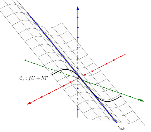
γa,b​(s)=(1−a2​s,a​s+b,(1+b​1−a2)​s)\gamma_{a,b}(s)=\big(\sqrt{1-a^{2}}\ s,as+b,(1+b\sqrt{1-a^{2}})s\big)

is the horizontally regular curve with horizontal arc-length. Since the projection of γ\gamma onto the x​yxy-plane is a line with slope a1−a2\frac{a}{\sqrt{1-a^{2}}}, the p-curvature κ≡0\kappa\equiv 0. We also have the contact normality τ≡1\tau\equiv 1. Set f⁡(t)=tf(t)=t, g⁡(t)≡0g(t)\equiv 0 and h⁡(t)=sin⁡(t)h(t)=\sin(t) for t∈[0,2​π]t\in[0,2\pi], then those functions satisfy the assumptions in Corollary 1.5 (2). In this case, we have the vectors U⁡(s)=(1−a2,a,b​1−a2)U(s)=\big(\sqrt{1-a^{2}},a,b\sqrt{1-a^{2}}\big), V⁡(s)=(−a,1−a2,−a​b−s)V(s)=\big(-a,\sqrt{1-a^{2}},-ab-s\big), and so the parametric surface is given by

𝕏⁡(s,t)\displaystyle\mathbb{X}(s,t) =γa,b+f​U+h​T\displaystyle=\gamma_{a,b}+fU+hT
=(1−a2​(s+t),a⁡(s+t)+b,b​1−a2​(s+t)+s+sin⁡(t)).\displaystyle=\Big(\sqrt{1-a^{2}}(s+t),a(s+t)+b,b\sqrt{1-a^{2}}(s+t)+s+\sin(t)\Big).

Note that the vector UU only depends on the number aa and the vector VV does not contribute to the surface, and so the surface Σ\Sigma is generated by the plane curve 𝒞s:f​U+h​T\mathcal{C}_{s}:fU+hT along the line γa,b\gamma_{a,b} as shown in Fig. 3.

Refer to caption
Figure 3. A plane satisfies Pappus-Guldin theorem for areas (Example 5.4 a=−0.9,b=0.5a=-0.9,b=0.5).

In [9] the author and the coauthors introduced the concept of the normal coordinates. More precisely, for any regular surface Σ=𝕏⁡(s,t)=γ⁡(s)+f⁡(t)​U​(s)+g⁡(t)​V​(s)\Sigma=\mathbb{X}(s,t)=\gamma(s)+f(t)U(s)+g(t)V(s), for any (s,t)∈D→ℍ1(s,t)\in D\rightarrow\mathbb{H}_{1} we can find the coordinates (called normal coordinates) such that the parametric equation of the surface satisfies that

  1. (1)

    𝕏⁡(D)\mathbb{X}(D) is a surface without singular points,

  2. (2)

    𝕏s\mathbb{X}_{s} defines the characteristic foliation on 𝕏⁡(D)\mathbb{X}(D),

  3. (3)

    |𝕏s|=1|\mathbb{X}_{s}|=1 on DD w.r.t. the Levi-metric.

Next we ask if the surfaces in Corollary 1.5 satisfying Pappus-Guldin theorem for areas can be the surface with constant p-mean curvature and the answer is positive. Recall that [6, Sec. 2, p. 134] the p-mean curvature HH of any surface Σ\Sigma is defined to be the variation of the p-area along the vector field e2=J​e1e_{2}=Je_{1} where e1e_{1} is the characteristic vector field Σ\Sigma. The p-mean curvature can also be represented by the function HH satisfying ∇e1e2=H​e2\nabla_{e_{1}}e_{2}=He_{2} (up to a sign) where ∇\nabla is the pseudo-hermitian connection. When using the normal coordinates, one has H=⟨𝕏t​t,J​𝕏t⟩H=\langle\mathbb{X}_{tt},J\mathbb{X}_{t}\rangle. Suppose γ⁡(s)\gamma(s) is parametrized by the horizontal arc-length and h⁡(t)≡0h(t)\equiv 0. Then the surface in Corollary 1.5 is given by 𝕏⁡(s,t)=γ+f​U+g​V\mathbb{X}(s,t)=\gamma+fU+gV and we have the derivatives

𝕏t\displaystyle\mathbb{X}_{t} =f′​U+g′​V=(f′​x′−g′​y′)​e̊1+(f′​y′+g′​x′)​e̊2,\displaystyle=f^{\prime}U+g^{\prime}V=(f^{\prime}x^{\prime}-g^{\prime}y^{\prime})\mathring{e}_{1}+(f^{\prime}y^{\prime}+g^{\prime}x^{\prime})\mathring{e}_{2},
𝕏t​t\displaystyle\mathbb{X}_{tt} =(f′′​x′−g′′​y′)​e̊1+(f′′​y′+g′′​y′)​e̊2.\displaystyle=(f^{\prime\prime}x^{\prime}-g^{\prime\prime}y^{\prime})\mathring{e}_{1}+(f^{\prime\prime}y^{\prime}+g^{\prime\prime}y^{\prime})\mathring{e}_{2}.

Thus, the p-mean curvature

(63) H\displaystyle H =⟨𝕏t​t,J​𝕏t⟩\displaystyle=\langle\mathbb{X}_{tt},J\mathbb{X}_{t}\rangle
=((x′)2+(y′)2)​(−f′′​g′+g′′​f′)\displaystyle=\Big((x^{\prime})^{2}+(y^{\prime})^{2}\Big)(-f^{\prime\prime}g^{\prime}+g^{\prime\prime}f^{\prime})
=−f′′​g′+g′′​f′.\displaystyle=-f^{\prime\prime}g^{\prime}+g^{\prime\prime}f^{\prime}.

Therefore by adding the constraint, −f′′​g′+g′′​f′=c​o​n​s​t.-f^{\prime\prime}g^{\prime}+g^{\prime\prime}f^{\prime}=const., we obtain the constant p-mean curvature surface and we summarize the result as follows.

Corollary 5.5.

When h⁡(t)≡0h(t)\equiv 0. For any functions f⁡(t),g⁡(t),κ⁡(s),τ⁡(s)f(t),g(t),\kappa(s),\tau(s) satisfying (f′)2+(g′)2=1(f^{\prime})^{2}+(g^{\prime})^{2}=1 and −f′′​g′+g′′​f′=C-f^{\prime\prime}g^{\prime}+g^{\prime\prime}f^{\prime}=C for some constant CC, then the surface Σ\Sigma defined by

(64) 𝕏⁡(s,t)=γ⁡(s)+f⁡(t)​U​(s)+g⁡(t)​V​(s)\displaystyle\mathbb{X}(s,t)=\gamma(s)+f(t)U(s)+g(t)V(s)

is a constant p-mean curvature with H=CH=C and its p-area is given by

𝒜⁡(Σ)=∫0s0∫0t0|τ⁡(s)−g⁡(t)|​𝑑t​𝑑s.\displaystyle\mathcal{A}(\Sigma)=\int_{0}^{s_{0}}\int_{0}^{t_{0}}|\tau(s)-g(t)|dtds.

In particular, if τ≡1>g\tau\equiv 1>g on [0,s0]×[0,t0][0,s_{0}]\times[0,t_{0}] (resp. τ≡−1<g\tau\equiv-1<g), then Pappus-Guldin theorem holds, namely,

𝒜⁡(Σ)\displaystyle\mathcal{A}(\Sigma) =s0​t0−s0​∫0t0g⁡(t)​𝑑t.\displaystyle=s_{0}t_{0}-s_{0}\int_{0}^{t_{0}}g(t)dt.
(resp.CLOSE\displaystyle(\text{resp. } OPEN=s0​t0+s0​∫0t0g⁡(t)​𝑑t)\displaystyle=s_{0}t_{0}+s_{0}\int_{0}^{t_{0}}g(t)dt)

Note that if the surface Σ\Sigma defined by (64) is a p-minimal surface (namely, H=0H=0), it does not bound any solid region. Indeed, by (63) the condition for being a p-minimal surface is that H=−f′′​g′+g′′​f′=0H=-f^{\prime\prime}g^{\prime}+g^{\prime\prime}f^{\prime}=0, and the condition holds if and only if f=C1​g+C2f=C_{1}g+C_{2} for some constants C1,C2C_{1},C_{2}. Thus, the curve 𝒞s​(t)=γ+f⁡(t)​U+g⁡(t)​V\mathcal{C}_{s}(t)=\gamma+f(t)U+g(t)V degenerates to a line segment such that the surface Σ\Sigma generated by 𝒞s​(t)\mathcal{C}_{s}(t) does not bound any solid region. The result has been observed in [6, Sec. 4]. The authors in that paper showed that the p-minimal surfaces are classical ruled surfaces with the ruled generated by Legendrian lines and clearly the ruled surfaces do not enclose any bounded region.

References

  • [1] C. B. Allendoerfer (1940) The euler number of a riemann manifold. American Journal of Mathematics 62 (1), pp. 243–248. Cited by: §1.
  • [2] Z. M. Balogh (2003) Size of characteristic sets and functions with prescribed gradient. Journal fur die Reine und Angewandte Mathematik, pp. 63–84. Cited by: §2.
  • [3] I. Bulmer-Thomas (1984) Guldin’s theorem–or pappus’s?. Isis 75 (2), pp. 348–352. Cited by: §1.
  • [4] L. Capogna, D. Danielli, and N. Garofalo (1994) An isoperimetric inequality and the geometric sobolev embedding for vector fields. Mathematical Research Letters 1 (2), pp. 263–268. Cited by: §2.
  • [5] S. Chang, C. Chen, and C. Wu (2018) On the cr analogue of reilly formula and yau eigenvalue conjecture. Asian Journal of Mathematics 22 (5), pp. 919 – 940. Cited by: §3.
  • [6] J. Cheng, J. Hwang, A. Malchiodi, and P. Yang (2005) Minimal surfaces in pseudohermitian geometry. Annali della Scuola Normale Superiore di Pisa-Classe di Scienze 4 (1), pp. 129–177. Cited by: §1, §1, §2, §3, §5, §5.
  • [7] J. Cheng, J. Hwang, and P. Yang (2007) Existence and uniqueness for p-area minimizers in the heisenberg group. Mathematische Annalen 337 (2), pp. 253–293. Cited by: §2, §2, Example 3.5.
  • [8] H. Chiu and P. T. Ho (2019) Global differential geometry of curves in three-dimensional heisenberg group and cr sphere. The Journal of Geometric Analysis 29 (4), pp. 3438–3469. Cited by: Remark 1.2, §2.
  • [9] H. Chiu, Y. Huang, and L. S. Lai (2017) An application of the moving frame method to integral geometry in the heisenberg group. Symmetry, Integrability and Geometry: Methods and Applications (SIGMA) 13 (097), pp. pp27. Cited by: §1, §2, §2, §2, §2, §3, §5.
  • [10] H. Chiu and S. Lai (2015) The fundamental theorem for hypersurfaces in heisenberg groups. Calculus of Variations and Partial Differential Equations 54 (1), pp. 1091–1118. Cited by: §1.
  • [11] G. Citti, B. Franceschiello, G. Sanguinetti, and A. Sarti (2016) Sub-riemannian mean curvature flow for image processing. SIAM Journal on Imaging Sciences 9 (1), pp. 212–237. Cited by: §2.
  • [12] W. Fenchel (1940) On total curvatures of riemannian manifolds: i. Journal of the London Mathematical Society 1 (1), pp. 15–22. Cited by: §1.
  • [13] H. Flanders (1970) A further comment on pappus. The American Mathematical Monthly 77 (9), pp. 965–968. Cited by: §1.
  • [14] B. Franchi, R. Serapioni, and F. S. Cassano (2001) Rectifiability and perimeter in the heisenberg group. Mathematische Annalen 321 (3), pp. 479–531. Cited by: §2.
  • [15] A.W. Goodman and G. Goodman (1969) Generalizations of the theorems of pappus. The American Mathematical Monthly 76 (4), pp. 355–366. Cited by: §1, §1, §1, §1, §1, §1, §1, §2.
  • [16] A. Gray and V. Miquel (2000) On pappus-type theorems on the volume in space forms. Annals of Global Analysis and Geometry 18 (3-4), pp. 241–254. Cited by: §1, §2.
  • [17] X. Gual-Arnau and V. Miquel (2006) Pappus-guldin theorems for weighted motions. Bulletin of the Belgian Mathematical Society-Simon Stevin 13 (1), pp. 123–137. Cited by: §1.
  • [18] L. Pursell (1970) More generalizations of a theorem of pappus. The American Mathematical Monthly 77 (9), pp. 961–965. Cited by: §1, §2.
  • [19] P. Radelet-de Grave (2015) Kepler, cavalieri, guldin. polemics with the departed. In Seventeenth-century indivisibles revisited, pp. 57–86. Cited by: §1.
  • [20] M. Ritoré and C. Rosales (2006) Rotationally invariant hypersurfaces with constant mean curvature in the heisenberg group hnh_{n}. The Journal of Geometric Analysis 16 (4), pp. 703. Cited by: §2.
  • [21] M. Ritoré and C. Rosales (2008) Area-stationary surfaces in the heisenberg group h1h_{1}. Advances in Mathematics 219 (2), pp. 633–671. Cited by: §2.
  • [22] G. Sanguinetti, G. Citti, and A. Sarti (2008) Implementation of a model for perceptual completion in r 2×\times s. In International conference on computer vision and computer graphics, pp. 188–201. Cited by: §2.
  • [23] R. W. Sharpe (2000) Differential geometry: cartan’s generalization of klein’s erlangen program. Vol. 166, Springer Science & Business Media. Cited by: §3.
  • [24] L. Vanhecke (1988) Geometry in normal and tubular neighborhoods. Rend. Sem. Fac. Sci. Univ. Cagliari, Supplement al 58, pp. 73–176. Cited by: §1.
  • [25] H. Weyl (1939) On the volume of tubes. American Journal of Mathematics 61 (2), pp. 461–472. Cited by: §1.