On the synthesis of control policies from noisy example datasets: a probabilistic approach

Davide Gagliardi Giovanni Russo Address: School of Electrical and Electronic Engineering, University College Dublin, Ireland (e-mail: davide.gagliardi@ucd.ie). Address: Department of Information and Electronic Engineering and Applied Mathematics, University of Salerno, Italy (e-mail: giovarusso@ucd.ie).

Abstract

In this note we consider the problem of synthesizing optimal control policies for a system from noisy datasets. We present a novel algorithm that takes as input the available dataset and, based on these inputs, computes an optimal policy for possibly stochastic and non-linear systems that also satisfies actuation constraints. The algorithm relies on solid theoretical foundations, which have their key roots into a probabilistic interpretation of dynamical systems. The effectiveness of our approach is illustrated by considering an autonomous car use case. For such use case, we make use of our algorithm to synthesize a control policy from noisy data allowing the car to merge onto an intersection, while satisfying additional constraints on the variance of the car speed.

1 Introduction

A framework that is becoming particularly appealing to design control algorithms is that of devising the control policy from examples (or demonstrations), see e.g. Hanawal et al. 2019; Wabersich and Zeilinger 2018 and references therein. At their roots these control from demonstration techniques, which are gaining considerable attention under the label of Inverse Reinforcement Learning (IRL), rely on Inverse Optimal Control and Optimization Bryson 1996. Today, IRL/control is recognized as an appealing framework to learn policies from success stories Argall et al. 2009 and potential applications include planning Englert et al. 2017 and preferences/prescriptions learning Xu and Paschalidis 2019.

There is then no surprise that, over the years, a number of techniques have been developed to address the problem of devising control policies from demonstrations, mainly in the context of Markov Decision Processes (MDPs) Sutton and Barto 1998. Results include Ratliff et al. 2009, which leverages a linear programming approach, Ratliff et al. 2006 which relies on a maximum margin approach, Ziebart et al. 2008 that makes use of the maximum entropy principle and Ramachandran and Amir 2007 that formalizes the problem via Bayesian statistics.

In this context, the main contributions of this extended abstract can be summarized as follows. First, we introduce an approach to synthesize control policies from examples which is based on the Fully Probabilistic Design (FPD) Kárný 1996; Kárný and Guy 2006; Herzallah 2015; Pegueroles and Russo 2019; Kárný and Kroupa 2012. This approach formalizes the control problem as an optimization problem where the Kullback-Leibler Divergence (see Section 2.2) between an ideal probability density function (pdf, obtained from e.g. demonstrations) and the pdf modeling the system/plant is minimized. The main technical novelty of our results with respect to the classic works on FPD lies in the fact that we explicitly embed actuation constraints in our formulation, thus solving an optimization problem where the Kullback-Leibler Divergence is minimized subject to constraints on the control variable. By relying on the FPD, one of the main advantages of our results over classic IRL/Control approaches is that policies can be synthesized from noisy data without requiring any assumption on the linearity of the system. The system can in fact be a general stochastic nonlinear dynamical system. Moreover, by embedding actuation constraints into the problem formulation and by solving the resulting optimization, we can export the policy that has been learned on other systems that have different actuation capabilities. As an additional contribution, we devise from our theoretical results an algorithmic procedure. The key reference applications over which the algorithm was tested involved an autonomous driving use case and full results are presented here.

2 Mathematical Preliminaries

2.1 Notation

Sets, as well as operators, are denoted by calligraphic characters, while vector quantities are denoted in bold. Let $n_{z}$ be a positive integer and consider the measurable space $(\mathcal{Z},\mathcal{F}_{z})$ , with $\mathcal{Z}\subseteq\mathbb{R}^{n_{z}}$ and with $\mathcal{F}_{z}$ being a $\sigma$ -algebra on $\mathcal{Z}$ . Then, the random vector (i.e. a multidimensional random variable) on $(\mathcal{Z},\mathcal{F}_{z})$ is denoted by $\mathbf{Z}$ and its realization is denoted by $\mathbf{z}$ (in the paper, we use the convention that these random vectors are row vectors). The probability density function (or simply pdf in what follows) of a continuous $\mathbf{Z}$ is denoted by $f_{\mathbf{Z}}(\mathbf{z})$ . For notational convenience, whenever it is clear from the context, we omit the argument and/or the subscript of the pdf. Hence, the support of $f:=f_{\mathbf{Z}}(\mathbf{z})$ is denoted by $\text{S}\left(f\right)$ and, analogously, the expectation of a function $\mathbf{h}(\cdot)$ of $\mathbf{Z}$ is indicated with $\mathbb{E}_{{f}}[\mathbf{h}(\mathbf{Z})]$ ad defined as $\mathbb{E}_{{f}}[\mathbf{h}(\mathbf{Z})]:=\int_{\text{S}\left(f\right)}\mathbf{h}(\mathbf{z})f(\mathbf{z})d\mathbf{z}$ . We also remark here that whenever we apply the averaging operator to a given function, we use an upper-case letter for the function argument as this is a random vector. The joint pdf of two random vectors, say $\mathbf{Z}$ and $\mathbf{Y}$ ,is denoted by $f_{\mathbf{[Z,Y]}}(\mathbf{z},\mathbf{y})$ and abbreviated with $f(\mathbf{z,y})$ . The conditional probability density function ( or cpdf in what follows) of $\mathbf{Z}$ with respect to the random vector $\mathbf{Y}$ is denoted by $f\left(\mathbf{z}|\mathbf{y}\right)$ and, whenever the context is clear, we use the shorthand notation $\tilde{f}_{\mathbf{Z}}$ . Finally, given $\mathcal{Z}\subseteq\mathbb{R}^{n_{z}}$ , its indicator function is denoted by $\mathds{1}_{\mathcal{Z}}(\mathbf{z})$ . That is, $\mathds{1}_{\mathcal{Z}}(\mathbf{z})=1$ , $\forall\mathbf{z}\in\mathcal{Z}$ and $0$ otherwise. We also make use of the internal product between tensors, which is denoted by $\langle\cdot,\cdot\rangle$ .

2.2 The Kullback-Leibler divergence

The control problem considered in this paper will be stated (see Section 3.1) in terms of the Kullback-Leibler (KL, Kullback and Leibler 1951) divergence, formalized with the following:

Definition 1 (Kullback-Leibler(KL) divergence)

Consider two pdfs, $\phi:=\phi_{\mathbf{Z}}(\mathbf{z})$ and $g:=g_{\mathbf{Z}}(\mathbf{z})$ , with $\phi$ being absolutely continuous with respect to $g$ . Then, the KL-divergence of $\phi$ with respect to $g$ is

\mathcal{D}_{\text{KL}}\left(\phi||g\right):=\int_{\text{S}(\phi)}\phi\;\ln\left(\frac{\phi}{g}\right)\,d\mathbf{z}.

(1)

Intuitively, $\mathcal{D}_{\text{KL}}\left(\phi||g\right)$ is a measure of how well $\phi$ approximates $g$ . We now give give a property of the KL-divergence, the KL-divergence splitting property, which is used in the proof of Theorem1.

Property 1

Let $\phi$ and $g$ be two pdfs of the random vector $[\mathbf{Z},\mathbf{Y}]$ , with $\mathbf{Z}$ and $\mathbf{Y}$ being random vectors of dimensions $n^{Z}$ and $n^{Y}$ , respectively. Then, the following splitting rule holds:

\begin{array}[]{l}\mathcal{D}_{\text{KL}}\left(\phi(\mathbf{y},\mathbf{z})||\,g(\mathbf{y},\mathbf{z})\right)=\\ \quad\mathcal{D}_{\text{KL}}\left(\phi(\mathbf{y})||\,g(\mathbf{y})\right)+\mathbb{E}_{\phi(\mathbf{Y})}\left[\mathcal{D}_{\text{KL}}\left(\phi(\mathbf{z}|\mathbf{Y})||\,g(\mathbf{z}|\mathbf{Y})\right)\right]\end{array}

(2)

Proof.

The proof follows from the definition of $\mathcal{D}_{\text{KL}}$ , the conditioning and independence rules for pdfs. A self-contained proof of this technical result is reported in the appendix. ∎

3 Formulation of the Control Problem

Let: (i) $\mathcal{K}:=\{k\}_{k=1}^{n}$ , $\mathcal{K}_{0}:=\mathcal{K}\cup\{0\}$ and $\mathcal{T}:=\{t_{k}:k\in\mathcal{K}_{0}\}$ be the time horizon over which the system is observed; (ii) $\mathbf{x}_{k}\in\mathbb{R}^{d_{x}}$ and $\mathbf{u}_{k}\in\mathbb{R}^{d_{u}}$ be, respectively, the system state and input at time $t_{k}\in\mathcal{T}$ ; (ii) $\mathbf{d}_{k}:=(\mathbf{x}_{k},\mathbf{u}_{k})$ be the data collected from the system at time $t_{k}\in\mathcal{T}$ and $\mathbf{d}^{k}$ the data collected from $t_{0}\in\mathcal{T}$ up to time $t_{k}\in\mathcal{T}$ ( $t_{k}>t_{0}$ ). As shown in e.g. Peterka 1981, the system behavior can be described via the joint pdf of the observed data, say $f(\mathbf{d}^{n})$ . Then, as shown in the same paper, the application of the chain rule for probability density functions leads to the following factorization for $f(\mathbf{d}^{n})$ :

f\left(\mathbf{d}^{n}\right)=\prod_{k\in\mathcal{K}}f\left(\mathbf{x}_{k}|\mathbf{u}_{k},\mathbf{x}_{k-1}\right)f\left(\mathbf{u}_{k}|\mathbf{x}_{k-1}\right)f\left(\mathbf{x}_{0}\right).

(3)

Throughout this work we refer to (3) as the probabilistic description of the closed loop system, or we simply say that (3) is our closed loop system.

Remark 1

The cpdf $f\left(\mathbf{x}_{k}|\mathbf{u}_{k},\mathbf{x}_{k-1}\right)$ describes the system behavior at time $t_{k}$ , given the previous state and the input at time $t_{k}$ . In turn, the input is also generated from the cdpf $f\left(\mathbf{u}_{k}|\mathbf{x}_{k-1}\right)$ , which is a randomized control policy, returning the input given the previous state. Finally, we also note that the initial conditions are embedded in the probabilistic system description through the prior $f\left(\mathbf{x}_{0}\right)$ .

In the rest of the paper we use the following shorthand notations: $\tilde{f}_{\mathbf{X}}^{k}:=f\left(\mathbf{x}_{k}|\mathbf{u}_{k},\mathbf{x}_{k-1}\right)$ , $\tilde{f}_{\mathbf{U}}^{k}:=f\left(\mathbf{u}_{k}|\mathbf{x}_{k-1}\right)$ , $f_{0}:=f\left(\mathbf{x}_{0}\right)$ and $f^{n}:=f\left(\mathbf{d}^{n}\right)$ . Hence, (3) can be compactly written as

f^{n}=\prod_{k\in\mathcal{K}}\tilde{f}_{\mathbf{X}}^{k}\tilde{f}_{\mathbf{U}}^{k}f_{0}=\tilde{f}^{n}f_{0},\ \ \ \tilde{f}^{n}:=\prod_{k\in\mathcal{K}}\tilde{f}_{\mathbf{X}}^{k}\tilde{f}_{\mathbf{U}}^{k}.

(4)

3.1 The control problem

Our goal is to synthesize, from an example dataset, say $\mathbf{d}_{e}^{n}$ , the control pdf $f\left(\mathbf{u}_{k}|\mathbf{x}_{k-1}\right)$ that allows the closed-loop system (4) to achieve the demonstrated behavior, subject to its actuation constraints. As in Kárný 1996; Quinn et al. 2016; Pegueroles and Russo 2019; Kárný and Guy 2006; Herzallah 2015 the behavior illustrated in the example dataset can be specified through the reference pdf $g\left(\mathbf{d}_{e}^{n}\right)$ extracted from the example dataset (as e.g. its empirical distribution). Following the chain rule for pdfs we have $g\left(\mathbf{d}_{e}^{n}\right):=\prod_{k\in\mathcal{K}}g\left(\mathbf{x}_{k}|\mathbf{u}_{k},\mathbf{x}_{k-1}\right)g\left(\mathbf{u}_{k}|\mathbf{x}_{k-1}\right)g\left(\mathbf{x}_{0}\right)$ . Again, by setting $\tilde{g}_{\mathbf{X}}^{k}:=g\left(\mathbf{x}_{k}|\mathbf{u}_{k},\mathbf{x}_{k-1}\right)$ , $\tilde{g}_{\mathbf{U}}^{k}:=g\left(\mathbf{u}_{k}|\mathbf{x}_{k-1}\right)$ , $g_{0}:=g\left(\mathbf{x}_{0}\right)$ and $g^{n}:=g\left(\mathbf{d}_{e}^{n}\right)$ we get:

g^{n}=\prod_{k\in\mathcal{K}}\tilde{g}_{\mathbf{X}}^{k}\tilde{g}_{\mathbf{U}}^{k}g_{0}=\tilde{g}^{n}g_{0},

(5)

where $\tilde{g}^{n}:=\prod_{k\in\mathcal{K}}\tilde{g}_{\mathbf{X}}^{k}\tilde{g}_{\mathbf{U}}^{k}$ .

The control problem can then be recast as the problem of designing $f\left(\mathbf{u}_{k}|\mathbf{x}_{k-1}\right)$ so that $f^{n}$ approximates $g^{n}$ . This leads to the following formalization:

Problem 1

Determine the sequence of cpdfs, say $\left\{\left(\tilde{f}_{\mathbf{U}}^{k}\right)^{*}\right\}_{k\in\mathcal{K}}$ , solving the nonlinear program

		$\displaystyle\underset{{\left\{\tilde{f}_{\mathbf{U}}^{k}\right\}_{k\in\mathcal{K}}}}{\min}$		$\displaystyle\mathcal{D}_{\text{KL}}\left(f^{n}\|\|g^{n}\right)$		(6)
		$\displaystyle\text{s.t.}$		$\displaystyle\mathbb{E}_{\tilde{f}_{\mathbf{U}}^{k}}\left[\tilde{\mathbf{h}}_{\mathbf{u},k}\left(\mathbf{U}\right)\right]=\tilde{\mathbf{H}}_{\mathbf{u},k},\quad k\in\mathcal{K},$		(6)

where the constraints are algebraically independent.

In Problem 1, the constraints are formalized as expectations. We note that these constraints can be equivalently written as $\int_{\text{S}(\tilde{f}_{\mathbf{U}}^{k})}\tilde{f}_{\mathbf{u}}^{k}\;\tilde{\mathbf{h}}_{\mathbf{u},k}\left(\mathbf{u}\right)\;d\mathbf{u}=\tilde{\mathbf{H}}_{\mathbf{u},k}$ . Also, the constraints of the program are time-varying and the number of constraints can change over time (the number of constraints at time $t_{k}$ is denoted by $c_{\mathbf{u},k}$ ). Indeed, in the constraints of (6): (i) $\tilde{\mathbf{H}}_{\mathbf{u},k}$ is a (column) vector of coefficients, i.e. $\tilde{\mathbf{H}}_{\mathbf{u},k}:=\left[H_{\mathbf{u},0,k},\mathbf{H}_{\mathbf{u},k}^{T}\right]^{T}$ and $\tilde{\mathbf{h}}_{\mathbf{u},k}\left(\mathbf{z}\right):=\left[h_{\mathbf{u},0,k},\mathbf{h}_{\mathbf{u},k}^{T}\right]^{T}(\mathbf{z})$ ; (ii) $\mathbf{H}_{\mathbf{u},k}\in\mathbb{R}^{c_{\mathbf{u},k}}$ and $\mathbf{h}_{\mathbf{u},k}:\text{S}(\tilde{f}_{\mathbf{u}}^{k})\mapsto\mathbb{R}^{c_{\mathbf{u},k}}$ ; (iii) $H_{\mathbf{u},0,k}:=1$ and $h_{\mathbf{u},0,k}\left(\mathbf{z}\right):=\mathds{1}_{\mathcal{U}_{k}}\left(\mathbf{z}\right)$ ensure that the solution of the program is a cpdf. Finally, in Problem 1 we assume that the constraints are algebraically independent. The notion of algebraically independent constraints is formalized next.

Definition 2

Let $\mathbf{Z}$ be a random vector with underlying pdf $f_{\mathbf{Z}}\left(\mathbf{z}\right)$ and support $\mathcal{Z}$ . A set of functions $\mathbf{h}:\mathcal{Z}\mapsto\mathbb{R}^{c_{\mathbf{z}}}$ is said to be algebraically independent if there exists a subset, say $S\subset\mathcal{Z}$ , with non-zero measure (i.e. $\int_{S}\,d\mathbf{z}>0$ ) and such that:

\exists S\subset\mathcal{Z}:\quad\int_{S}\langle\mathbf{v},\,\mathbf{h}\left(\mathbf{z}\right)\rangle^{2}\,d\mathbf{z}>0,\quad\forall\mathbf{v}\in\mathbb{R}^{c_{\mathbf{z}}}\backslash{\mathbf{0}}

(7)

In what follows, we simply say that a set of equations (or constraints) of the form of (7) is algebraically independent if the above definition is satisfied. As shown in Guilleminot and Soize 2013, the assumption that the contraints are algebraically independent ensures that Problem 1 is well posed.

4 Technical Results

We now introduce the main technical results of this paper. The key result behind the algorithm of Section 5 is Theorem 1. The proof of this result, given in this section, makes use of three technical lemmas (i.e. Lemma 1, Lemma 2 and Lemma3).

Lemma 1

Let: (i) $\mathbf{Z}$ be a random vector on the measurable space $\left(\mathcal{Z},\mathcal{F}_{z}\right)$ ; (ii) $f:=f_{\mathbf{Z}}(\mathbf{z})$ , $g:=g_{\mathbf{Z}}(\mathbf{z})$ be two probability distributions over $\left(\mathcal{Z},\mathcal{F}_{z}\right)$ ; (iii) $\alpha:\mathcal{Z}\mapsto\mathbb{R}_{0}^{+}$ be a nonnegative function of $\mathbf{Z}$ , integrable under the measure given by $f_{\mathbf{Z}}(\mathbf{z})$ . Assume that $f_{\mathbf{Z}}(\mathbf{z})$ satisfies the following set of algebraically independent equations:

\begin{array}[]{lrl}\int{f_{\mathbf{Z}}\left(\mathbf{z}\right)\;\tilde{\mathbf{h}}\left(\mathbf{z}\right)\;d\mathbf{z}}=\tilde{\mathbf{H}},\end{array}

(8)

where: (i) $\tilde{\mathbf{h}}(\mathbf{z}):=\left[h_{0},\mathbf{h}^{T}\right]^{T}(\mathbf{z})$ , with $h_{0}(\mathbf{z}):=\mathds{1}_{\mathcal{S}\left(\mathbf{Z}\right)}(\mathbf{z})$ and $\mathbf{h}:\mathcal{Z}\mapsto\mathbb{R}^{c_{\mathbf{z}}}$ being a measurable map; (ii) $\tilde{\mathbf{H}}(\mathbf{z}):=\left[H_{0},\mathbf{H}^{T}\right]^{T}$ with $H_{0}:=1$ and $\mathbf{H}\in\mathbb{R}^{c_{\mathbf{z}}}$ being a vector of constants. Then:

the solution of the constrained optimization problem

\displaystyle\underset{f_{\mathbf{Z}}}{\min}

\displaystyle\mathcal{L}(f)

\displaystyle\text{s.t.}

\displaystyle\text{constraints in \eqref{eq:gen_constr}}

(9)

with

\mathcal{L}(f):=\mathcal{D}_{\text{KL}}\left(f||g\right)+\int f_{\mathbf{Z}}(\mathbf{z})\;\alpha\left(\mathbf{z}\right)\,d\mathbf{z}

(10)

is the pdf

f^{\ast}:=f^{\ast}_{\mathbf{Z}}\left(\mathbf{z}\right)=\frac{g\left(\mathbf{z}\right)e^{-\{\alpha\left(\mathbf{z}\right)+\langle\boldsymbol{\lambda}^{*},\mathbf{h}\left(\mathbf{z}\right)\rangle\}}}{e^{1+\lambda^{*}_{0}}}.

(11)

In (11) $\lambda^{\ast}_{0}$ and $\boldsymbol{\lambda}^{\ast}=[\lambda^{\ast}_{1},\dots,\lambda^{\ast}_{c_{\mathbf{z}}}]^{T}$ are the Lagrange multipliers associated to the constraints;

moreover, the corresponding minimum is:

\mathcal{L}^{\ast}:=\mathcal{L}\left(f^{*}\right)=-\left(1+\lambda^{\ast}_{0}+\langle\boldsymbol{\lambda}^{\ast},\mathbf{H}\rangle\right).

(12)

Proof.

See the appendix. ∎

Note that, in Lemma 1, the optimal solution $f_{\mathbf{Z}}^{\ast}(\mathbf{z})$ depends on the Lagrange multipliers (LMs) $\lambda_{0}^{\ast}$ and $\boldsymbol{\lambda}^{\ast}$ . The first LM, i.e. $\lambda_{0}^{\ast}$ , can be obtained by integration, i.e. by imposing that $e^{1+\lambda_{0}^{\ast}}$ normalizes $f_{\mathbf{Z}}^{\ast}(\mathbf{z})$ in (11). With the next result, we propose a strategy for finding the LMs $\boldsymbol{\lambda}^{\ast}$ . In particular, the idea is to recast the problem of finding the solutions of non-linear equations as a minimization problem. In general, the approach can be also used to fit the parameters of a pdf so that it meets a set of pre-specified constrains (for example, to find pdfs that satisfy the Maximum Entropy principle Guilleminot and Soize 2013).

Lemma 2

Let: (i) $\mathcal{Z}\subseteq\mathbb{R}^{n_{\mathbf{z}}}$ and $\tilde{\Theta}\subseteq\mathbb{R}^{n_{\mathbf{z}}}$ ; (ii) $\hat{f}_{1}:\mathcal{Z}\mapsto\hat{f}_{1}\left(\mathbf{z}\right)$ be a positive and integrable function on $\mathcal{Z}$ ; (iii) $\hat{f}_{2}:(\mathcal{Z}\times\tilde{\Theta})\mapsto\hat{f}_{1}\left(\mathbf{z}\right)e^{-\langle\tilde{\boldsymbol{\theta}},\;\tilde{\mathbf{h}}\left(\mathbf{z}\right)\rangle}$ , where $\tilde{\mathbf{h}}=\left[\tilde{\mathbf{h}}_{1}\left(\mathbf{z}\right),\ldots,\tilde{\mathbf{h}}_{c_{\mathbf{z}}}\left(\mathbf{z}\right)\right]^{T}:\mathcal{Z}\mapsto\mathbb{R}^{c_{\mathbf{z}}}$ are algebraically independent functions. Consider the constraints defined by the set of the following equations:

\int_{\mathcal{Z}}\hat{f}_{2}\left(\mathbf{z},\tilde{\boldsymbol{\theta}}\right)\tilde{\mathbf{h}}_{i}\left(\mathbf{z}\right)\;d\mathbf{z}=\tilde{\mathbf{H}}_{i},\;\quad i=1,\dots,c_{\mathbf{z}},

(13)

where $\tilde{\mathbf{H}}:=\left[\tilde{\mathbf{H}}_{1},\ldots,\tilde{\mathbf{H}}_{c_{\mathbf{z}}}\right]^{T}\in\mathbb{R}^{c_{\mathbf{z}}}$ . Then, the unique solution, say $\tilde{\boldsymbol{\theta}}^{\ast}$ , of the minimization problem

\underset{\tilde{\boldsymbol{\theta}}}{\min}\;\mathcal{J}\left(\tilde{\boldsymbol{\theta}}\right),

(14)

with $\mathcal{J}\left(\tilde{\boldsymbol{\theta}}\right):=\langle\tilde{\boldsymbol{\theta}},\,\tilde{\mathbf{H}}\rangle+\int_{\mathcal{Z}}\hat{f}_{2}\left(\mathbf{z},\tilde{\boldsymbol{\theta}}\right)\,d\mathbf{z}$ is also a solution of (13).

Proof.

See the appendix ∎

Finally, we introduce here the following technical lemma that is used in the proof of Theorem 1.

Lemma 3

Let $f^{n}$ and $g^{n}$ be the pdfs defined in (3) and (5), respectively. Then:

\mathcal{D}_{\text{KL}}\left(f^{n}||g^{n}\right)=\mathcal{D}_{\text{KL}}\left(f^{n-1}||g^{n-1}\right)+\mathbb{E}_{f^{n-1}}\left[\mathcal{D}_{\text{KL}}\left(\tilde{f}^{n}||\tilde{g}^{n}\right)\right]

(15)

Proof.

The result is obtained from Property 1 (see the appendix for a proof of this property) by setting $\mathbf{Y}:=[\mathbf{X}_{0},\mathbf{U}_{1},\mathbf{X}_{1},\dots,\mathbf{U}_{n-1},\mathbf{X}_{n-1}]$ and $\mathbf{Z}:=[\mathbf{U}_{n},\mathbf{X}_{n}]$ ∎

The main result behind the algorithm of Section 5, the proof of which makes use of the above technical results, is presented next.

Theorem 1

The solution, $\left(\tilde{f}_{\mathbf{U}}^{k}\right)^{\ast}=f^{\ast}\left(\mathbf{u}_{k}|\mathbf{x}_{k-1}\right)$ , of the control Problem 1 is

\left(\tilde{f}_{\mathbf{U}}^{k}\right)^{*}=\tilde{g}_{\mathbf{U}}^{k}\frac{e^{-\{\hat{\omega}\left(\mathbf{u}_{k},\,\mathbf{x}_{k-1}\right)+\langle\boldsymbol{\lambda}^{*}_{\mathbf{u},k},\mathbf{h}_{\mathbf{u},k}\left(\mathbf{u}_{k}\right)\rangle\}}}{e^{1+\lambda^{*}_{\mathbf{u},0,k}}},

(16)

where:

$\hat{\omega}(\cdot,\cdot)$ is generated via the backward recursion

\hat{\omega}\left(\mathbf{u}_{k},\,\mathbf{x}_{k-1}\right)=\hat{\alpha}\left(\mathbf{u}_{k},\,\mathbf{x}_{k-1}\right)+\hat{\beta}\left(\mathbf{u}_{k},\,\mathbf{x}_{k-1}\right),

(17)

with

\begin{split}\hat{\alpha}\left(\mathbf{u}_{k},\,\mathbf{x}_{k-1}\right)&:=\mathcal{D}_{\text{KL}}\left(\tilde{f}^{k}_{\mathbf{X}}||\tilde{g}^{k}_{\mathbf{X}}\right)\\ \hat{\beta}\left(\mathbf{u}_{k},\,\mathbf{x}_{k-1}\right)&:=-\mathbb{E}_{\tilde{f}^{k}_{\mathbf{X}}}\left[\ln\hat{\gamma}\left(\mathbf{X}_{k}\right)\right],\end{split}

(18)

with terminal conditions $\hat{\beta}\left(\mathbf{u}_{n},\,\mathbf{x}_{n-1}\right)=0$ and $\hat{\alpha}\left(\mathbf{u}_{n},\,\mathbf{x}_{n-1}\right)=\mathcal{D}_{\text{KL}}\left(\tilde{f}^{n}_{\mathbf{X}}||\tilde{g}^{n}_{\mathbf{X}}\right)$ ;

$\hat{\gamma}\left(\cdot\right)$ in (18) is given by

\ln\hat{\gamma}\left(\mathbf{x}_{k-1}\right):=\left[\sum_{i=0}^{c_{\mathbf{u}}}\ln\left(\hat{\gamma}_{\mathbf{u},i,k}\left(\mathbf{x}_{k-1}\right)\right)\right],

(19)

with

\hat{\gamma}_{\mathbf{u},0,k}\left(\mathbf{x}_{k-1}\right)=\exp{\{\lambda^{*}_{\mathbf{u},0,k}+1\}},

(20)

and

\hat{\gamma}_{\mathbf{u},i,k}\left(\mathbf{x}_{k-1}\right):=\exp{\{\lambda^{*}_{\mathbf{u},i,k}\mathbf{H}_{\mathbf{u},i,k}\}}\quad i=1,\dots,c_{\mathbf{u}},

(21)

with terminal conditions $\hat{\gamma}_{\mathbf{u},0,n}\left(\mathbf{x}_{n-1}\right)=1$ , i.e. $\lambda^{*}_{\mathbf{u},0,n}=0$ , and $\lambda^{\ast}_{\mathbf{u},i,n}=0$ , $i=1,\ldots,n$ ;

$\lambda^{\ast}_{\mathbf{u},0,k}$ and $\boldsymbol{\lambda}^{\ast}_{\mathbf{u},k}=\left[\lambda_{\mathbf{u},1,k}^{\ast},\dots,\lambda_{\mathbf{u},c_{\mathbf{u}},k}^{\ast}\right]$ in (16) are the Lagrange multipliers (LMs) associated to the constraints at time $t_{k}$ . In particular,

\begin{split}&\lambda^{\ast}_{\mathbf{u},0,k}=\\ &\ln\left[\int\tilde{g}_{\mathbf{U}}^{k}\left(e^{-\{\hat{\omega}\left(\mathbf{u}_{k},\,\mathbf{x}_{k-1}\right)+\langle\boldsymbol{\lambda}^{*}_{\mathbf{u},k},\mathbf{h}_{\mathbf{u},k}\left(\mathbf{u}_{k}\right)\rangle\}}\right)\;d\mathbf{u}_{k}\right]-1,\end{split}

while all the other LMs can be obtained numerically (via e.g. Lemma 2).

Moreover, the corresponding minimum at time $k$ is given by:

B^{*}_{k}:=-\mathbb{E}_{p^{k-1}_{\mathbf{X}}}\left[\ln\hat{\gamma}\left(\mathbf{X}_{k-1}\right)\right].

(22)

where $p_{\mathbf{X}}^{k}$ denotes the pdf of the state at time $t_{k}$ (i.e. $p_{\mathbf{X}}^{k}:=f\left(\mathbf{x}_{k}\right)$ ).

Proof.

For notational convenience, we use the shorthand notation $\left\{\mathbf{E}_{\mathbf{u},k}\right\}$ to denote the set of constraints of Problem 1 at time $t_{k}$ . We also denote by $\left\{\mathbf{E}_{\mathbf{u},k}\right\}_{\mathcal{K}}$ the set of constraints over the whole time horizon $\mathcal{K}$ and $\left\{\mathbf{E}_{\mathbf{u},k}\right\}_{k=1}^{n-1}$ to denote the constraints from $t_{1}$ up to time $t_{n-1}$ .

Note that, following Lemma 3, Problem 1 can be re-written as follows:

\begin{array}[]{l}\underset{\footnotesize\begin{array}[]{l}\left\{\tilde{f}_{\mathbf{U}}^{k}\right\}_{k\in\mathcal{K}}\\ \text{ s.t.:}\\ \left\{\mathbf{E}_{\mathbf{u},k}\right\}_{k\in\mathcal{K}}\end{array}}{\min}\mathcal{D}_{\text{KL}}\left(f^{n}||g^{n}\right)=\\ \qquad=\underset{\footnotesize\begin{array}[]{l}\left\{\tilde{f}_{\mathbf{U}}^{k}\right\}_{k=1}^{n-1}\\ \text{ s.t.:}\\ \left\{\mathbf{E}_{\mathbf{u},k}\right\}_{k=1}^{n-1}\end{array}}{\min}\left\{\mathcal{D}_{\text{KL}}\left(f^{n-1}||g^{n-1}\right)+B^{*}_{n}\right\}\\ \end{array}

(23)

where:

B^{*}_{n}:=\underset{\footnotesize\begin{array}[]{l}\tilde{f}_{\mathbf{U}}^{n}\\ \text{ s.t.:}\\ \mathbf{E}_{\mathbf{u},n}\end{array}}{\min}B_{n}\,,\quad B_{n}:=\mathbb{E}_{f^{n-1}}\left[\mathcal{D}_{\text{KL}}\left(\tilde{f}^{n}||\tilde{g}^{n}\right)\right].

(24)

That is, Problem 1 can be approached by solving first the optimization of the last time-instant of the time-horizon $\mathcal{K}$ (the term $B_{n}$ in (23)) and then by taking into account the result from this optimization problem in the optimization up to the instant $t_{n-1}$ . Now we focus on the sub-problem:

B^{*}_{n}:=\underset{\footnotesize\begin{array}[]{l}\tilde{f}_{\mathbf{U}}^{n}\\ \text{ s.t.:}\\ \mathbf{E}_{\mathbf{u},n}\end{array}}{\min}B_{n}

(25)

For this problem, we first observe that the following equality is satisfied for the term $B_{n}$ :

B_{n}=\mathbb{E}_{f^{n-1}}\left[\mathcal{D}_{\text{KL}}\left(\tilde{f}^{n}||\tilde{g}^{n}\right)\right]=\mathbb{E}_{p^{n-1}_{\mathbf{X}}}\left[\mathcal{D}_{\text{KL}}\left(\tilde{f}^{n}||\tilde{g}^{n}\right)\right].

(26)

Such equality was obtained by noting that $\mathcal{D}_{\text{KL}}\left(\tilde{f}^{n}||\tilde{g}^{n}\right)$ is only a function of the previous state (see also Kárný 1996) and, for notational convenience, we rename it as $\hat{A}\left(\cdot\right)$ . Hence, $B_{n}$ becomes

B_{n}=\mathbb{E}_{p^{n-1}_{\mathbf{X}}}\left[\mathcal{D}_{\text{KL}}\left(\tilde{f}^{n}||\tilde{g}^{n}\right)\right]=\mathbb{E}_{p^{n-1}_{\mathbf{X}}}\left[\hat{A}\left(\mathbf{X}_{n-1}\right)\right].

(27)

Now, note that

\begin{array}[]{ll}B^{*}_{n}:&=\underset{\footnotesize\begin{array}[]{l}\tilde{f}_{\mathbf{U}}^{n}\\ \text{ s.t.:}\\ \mathbf{E}_{\mathbf{u},n}\end{array}}{\min}B_{n}=\underset{\footnotesize\begin{array}[]{l}\tilde{f}_{\mathbf{U}}^{n}\\ \text{ s.t.:}\\ \mathbf{E}_{\mathbf{u},n}\end{array}}{\min}\mathbb{E}_{p^{n-1}_{\mathbf{X}}}\left[\hat{A}\left(\mathbf{X}_{n-1}\right)\right]=\\ &=\mathbb{E}_{p^{n-1}_{\mathbf{X}}}\left[\underset{\footnotesize\begin{array}[]{l}\tilde{f}_{\mathbf{U}}^{n}\\ \text{ s.t.:}\\ \mathbf{E}_{\mathbf{u},n}\end{array}}{\min}\hat{A}\left(\mathbf{X}_{n-1}\right)\right]=\mathbb{E}_{p^{n-1}_{\mathbf{X}}}\left[A^{*}_{n}\right],\end{array}

(28)

where the above expression was obtained by using the fact that the expectation operator is linear and the fact that independence of the decision variable (i.e. $\tilde{f}_{\mathbf{U}}^{n}$ ) is independent on the pdf over which the expectation is performed (i.e. $p^{n-1}_{\mathbf{X}}$ ). This implies that, once we solve the problem

A^{\ast}_{n}:=\underset{\footnotesize\begin{array}[]{l}\tilde{f}_{\mathbf{u}}^{n}\\ \text{ s.t.:}\\ \mathbf{E}_{\mathbf{u},n}\end{array}}{\min}\hat{A}(\mathbf{x}_{n-1})

(29)

for any fixed $\mathbf{x}_{n-1}$ , then $B^{*}_{n}$ can be obtained by averaging $A^{\ast}_{n}$ over $p_{\mathbf{X}}^{n-1}$ . We now focus on solving problem (29). In doing so, we first note that, following (27), $\hat{A}(\mathbf{x}_{n-1})$ can be re-written as follows:

	$\hat{A}\left(\mathbf{x}_{n-1}\right)=\int\tilde{f}^{n}_{\mathbf{U}}\left[\ln\left(\frac{\tilde{f}^{n}_{\mathbf{U}}}{\tilde{g}^{n}_{\mathbf{U}}}\right)+\hat{\alpha}\left(\mathbf{u}_{n},\mathbf{x}_{n-1}\right)\right]\,d\mathbf{u}_{n},$		(30a)
	$\hat{\alpha}\left(\mathbf{u}_{n},\mathbf{x}_{n-1}\right):=\mathcal{D}_{\text{KL}}\left(\tilde{f}^{n}_{\mathbf{X}}\|\|\tilde{g}^{n}_{\mathbf{X}}\right).$		(30b)

In turn, (30a) can be compactly written as:

\hat{A}(\mathbf{x}_{n-1})=\mathcal{D}_{\text{KL}}\left(\tilde{f}_{u}^{n}||\tilde{g}_{u}^{n}\right)+\int{\tilde{f}_{\mathbf{U}}^{n}\,\hat{\alpha}\left(\mathbf{u}_{n},\mathbf{x}_{n-1}\right)\,d\mathbf{u}_{n}},

(31)

where we used the definition of KL-divergence. Hence, Lemma 1 can be used to solve the optimization problem in.(29). Indeed by applying Lemma 1 with $\mathbf{Z}=\mathbf{U}_{n}$ , $f=\tilde{f}_{\mathbf{U}}^{n}$ , $g=\tilde{g}_{\mathbf{U}}^{n}$ , $\mathbf{h}=\mathbf{h}_{\mathbf{u},n}$ , $\mathbf{H}=\mathbf{H}_{\mathbf{u},n}$ we get the following solution to (29):

\left(\tilde{f}_{\mathbf{U}}^{n}\right)^{\ast}=\tilde{g}_{\mathbf{U}}^{n}\frac{e^{-\{\hat{\alpha}\left(\mathbf{u}_{n},\,\mathbf{x}_{n-1}\right)+\langle\boldsymbol{\lambda}^{\ast}_{\mathbf{u},n},\mathbf{h}_{\mathbf{u},n}\left(\mathbf{u}_{n}\right)\rangle\}}}{e^{1+\lambda^{\ast}_{\mathbf{u},0,n}}}.

(32)

In the above pdf, $\lambda^{\ast}_{\mathbf{u},0,n}$ and $\boldsymbol{\lambda}^{\ast}_{\mathbf{u},n}$ are the LMs at the last time instant, $t_{n}$ . The LM $\lambda^{\ast}_{\mathbf{u},0,n}$ can be obtained by imposing a normalization condition to (32). That is, $\lambda^{\ast}_{\mathbf{u},0,n}$ can be found by imposing that

\begin{array}[]{ll}\exp\{\lambda^{*}_{\mathbf{u},0,n}+1\}&=\int\tilde{g}_{\mathbf{U}}^{n}e^{-\{\hat{\alpha}\left(\mathbf{u}_{n},\,\mathbf{x}_{n-1}\right)+\langle\boldsymbol{\lambda}^{*}_{\mathbf{u},n},\mathbf{h}_{\mathbf{u},n}\left(\mathbf{u}_{n}\right)\rangle\}}\;d\mathbf{u}_{n}\\ &=\hat{\gamma}_{\mathbf{u},0,n}\left(\mathbf{x}_{n-1}\right).\end{array}

(33)

Also, following Lemma 1, the minimum of the problem is given by:

\hat{A}^{\ast}_{n}=-\left(1+\lambda^{\ast}_{\mathbf{u},0,n}+\langle\boldsymbol{\lambda}^{\ast}_{\mathbf{u},n},\mathbf{H}_{\mathbf{u},n}\rangle\right)

(34)

or equivalently

\hat{A}^{\ast}_{n}=-\left[\sum_{i=0}^{c_{\mathbf{u}}}\ln\left(\hat{\gamma}_{\mathbf{u},i,n}\left(\mathbf{x}_{n-1}\right)\right)\right]=-\ln\hat{\gamma}\left(\mathbf{x}_{n-1}\right)

(35)

where we have used the definitions (20) and (21) for $\hat{\gamma}_{\mathbf{u},i,n},i=0,\dots c_{\mathbf{u}}$ . Therefore, the corresponding minimum value for $B_{n}$ is:

B^{\ast}_{n}=-\mathbb{E}_{p^{n-1}_{\mathbf{X}}}\left[\ln\hat{\gamma}\left(\mathbf{X}_{n-1}\right)\right].

(36)

Note now that the solution we found to the problem in (25) only depends on $\mathbf{X}_{n-1}$ and therefore the original problem (23) can be split as

\begin{array}[]{ll}\underset{\footnotesize\begin{array}[]{l}\left\{\tilde{f}_{\mathbf{U}}^{k}\right\}_{k=1}^{n-1}\\ \text{ s.t.:}\\ \left\{\mathbf{E}_{\mathbf{u},k}\right\}_{k=1}^{n-1}\end{array}}{\min}&\left\{\mathcal{D}_{\text{KL}}\left(f^{n-1}||g^{n-1}\right)+B^{*}_{n}\right\}=\\ \quad=\underset{\footnotesize\begin{array}[]{l}\left\{\tilde{f}_{\mathbf{U}}^{k}\right\}_{k=1}^{n-2}\\ \text{ s.t.:}\\ \left\{\mathbf{E}_{\mathbf{u},k}\right\}_{k=1}^{n-2}\end{array}}{\min}&\left\{\mathcal{D}_{\text{KL}}\left(f^{n-2}||g^{n-2}\right)+B^{*}_{n-1}\right\}\\ \\ \end{array}

(37)

where:

	$B^{*}_{n-1}:=\underset{\footnotesize\begin{array}[]{l}\tilde{f}_{\mathbf{U}}^{n-1}\\ \text{ s.t.:}\\ \mathbf{E}_{\mathbf{u},n-1}\end{array}}{\min}B_{n-1},$		(38a)
	$B_{n-1}:=\mathbb{E}_{f^{n-2}}\left[\mathcal{D}_{\text{KL}}\left(\tilde{f}^{n-1}\|\|\tilde{g}^{n-1}\right)\right]+B^{\ast}_{n}$		(38b)

We approach the above problem in the same way we used to solve the problem in (25). The idea is now to find a function, $\hat{A}\left(\mathbf{x}_{n-2}\right)$ , such that

B_{n-1}=\mathbb{E}_{p^{n-2}_{\mathbf{X}}}\left[\hat{A}\left(\mathbf{X}_{n-2}\right)\right].

(39)

Once this is done, we then solve the problem

A^{*}_{n-1}:=\underset{\footnotesize\begin{array}[]{l}\tilde{f}_{\mathbf{U}}^{n}\\ \text{ s.t.:}\\ \mathbf{E}_{\mathbf{u},n}\end{array}}{\min}\hat{A}(\mathbf{x}_{n-2})

(40)

and obtain $B^{*}_{n-1}$ as

B^{*}_{n-1}\begin{array}[]{ll}:=\mathbb{E}_{p^{n-2}_{\mathbf{X}}}\left[A^{*}_{n-1}\right].\end{array}

(41)

To this end we first note that the following identities

	$\mathbb{E}_{p^{n-1}_{\mathbf{X}}}\left[\varphi\left(\mathbf{X}_{n-1}\right)\right]=\mathbb{E}_{p^{n-2}_{\mathbf{X}}}\left[\mathbb{E}_{\tilde{f}^{n-1}}\left[\varphi\left(\mathbf{X}_{n-1}\right)\right]\right]$		(42a)
	$\mathbb{E}_{\tilde{f}^{n-1}_{\mathbf{X}}}\left[\varphi\left(\mathbf{X}_{n-1}\right)\right]=\mathbb{E}_{\tilde{f}^{n-2}_{\mathbf{X}}}\left[\mathbb{E}_{\tilde{f}^{n-1}}\left[\varphi\left(\mathbf{X}_{n-1}\right)\right]\right]$		(42b)

hold for any function $\varphi$ of $\mathbf{X}_{n-1}$ . Therefore, by means of (36) and (42a) we obtain, from (38b):

\begin{array}[]{l}B_{n-1}=\mathbb{E}_{f^{n-2}}\left[\mathcal{D}_{\text{KL}}\left(\tilde{f}^{n-1}||\tilde{g}^{n-1}\right)\right]+B^{\ast}_{n}=\\ =\mathbb{E}_{p^{n-2}_{\mathbf{X}}}\left[\mathcal{D}_{\text{KL}}\left(\tilde{f}^{n-1}||\tilde{g}^{n-1}\right)\right]+B^{\ast}_{n}=\\ =\mathbb{E}_{p^{n-2}_{\mathbf{X}}}\left[\mathcal{D}_{\text{KL}}\left(\tilde{f}^{n-1}||\tilde{g}^{n-1}\right)\right]+\\ \qquad-\mathbb{E}_{p^{n-2}_{\mathbf{X}}}\left[\mathbb{E}_{\tilde{f}^{n-1}}\left[\ln\hat{\gamma}\left(\mathbf{X}_{n-1}\right)\right]\right]=\\ =\mathbb{E}_{p^{n-2}_{\mathbf{x}}}\left[\underbrace{\mathcal{D}_{\text{KL}}\left(\tilde{f}^{n-1}||\tilde{g}^{n-1}\right)+\mathbb{E}_{\tilde{f}^{n-1}}\left[-\ln\hat{\gamma}\left(\mathbf{X}_{n-1}\right)\right]}_{=:\hat{A}\left(\mathbf{X}_{n-2}\right)}\right]\end{array}

(43)

and the term $\hat{A}\left(\mathbf{x}_{n-2}\right)$ can be recognized. Now, following the same reasoning we used to compute $\hat{A}(\mathbf{x}_{n-1})$ , we explicitly write $\hat{A}(\mathbf{x}_{n-2})$ in compact form as

\begin{array}[]{ll}\hat{A}\left(\mathbf{x}_{n-2}\right)=\\ =\mathcal{D}_{\text{KL}}\left(\tilde{f}^{n-1}||\tilde{g}^{n-1}\right)+\mathbb{E}_{\tilde{f}^{n-1}_{\mathbf{U}}}\left[\mathbb{E}_{\tilde{f}^{n-1}_{\mathbf{X}}}\left[-\ln\hat{\gamma}\left(\mathbf{X}_{n-1}\right)\right]\right]=\\ =\int\tilde{f}^{n-1}_{\mathbf{U}}\left\{\ln\left(\frac{\tilde{f}^{n-1}_{\mathbf{U}}}{\tilde{g}^{n-1}_{\mathbf{U}}}\right)+\hat{\omega}\left(\mathbf{u}_{n-1},\,\mathbf{x}_{n-2}\right)\right\}\,d\mathbf{u}_{n-1}\,,\end{array}

(44)

where $\hat{\omega}\left(\mathbf{u}_{n-1},\,\mathbf{x}_{n-2}\right)=\hat{\alpha}\left(\mathbf{u}_{n-1},\,\mathbf{x}_{n-2}\right)+\hat{\beta}\left(\mathbf{u}_{n-1},\,\mathbf{x}_{n-2}\right)$ and

\begin{array}[]{rll}\hat{\alpha}\left(\mathbf{u}_{n-1},\,\mathbf{x}_{n-2}\right)&:=\mathcal{D}_{\text{KL}}\left(\tilde{f}^{n-1}_{\mathbf{X}}||\tilde{g}^{n-1}_{\mathbf{X}}\right)\\ \hat{\beta}\left(\mathbf{u}_{n-1},\,\mathbf{x}_{n-2}\right)&:=-\mathbb{E}_{\tilde{f}^{n-1}_{\mathbf{X}}}\left[\ln\hat{\gamma}\left(\mathbf{X}_{n-1}\right)\right]\\ \end{array}

(45)

The last expression for $\hat{A}(\mathbf{x}_{n-2})$ obtained in (44) allows us to use the Lemma 1 to solve the optimization problem defined in (40). Indeed by applying Lemma 1 with $\mathbf{Z}=\mathbf{U}_{n-1}$ , $f=\tilde{f}_{\mathbf{U}}^{n-1}$ , $g=\tilde{g}_{\mathbf{U}}^{n-1}$ , $\mathbf{h}=\mathbf{h}_{\mathbf{u},n-1}$ , $\mathbf{H}=\mathbf{H}_{\mathbf{u},n-1}$ , $\hat{\alpha}(\cdot)=\hat{\omega}(\cdot)$ , we get the following solution to the problem in (40):

\left(\tilde{f}_{\mathbf{U}}^{n-1}\right)^{\ast}=\tilde{g}_{\mathbf{U}}^{n-1}\frac{e^{-\{\hat{\omega}\left(\mathbf{u}_{n-1},\,\mathbf{x}_{n-2}\right)+\langle\boldsymbol{\lambda}^{*}_{\mathbf{u},n-1},\mathbf{h}_{\mathbf{u},n-1}\left(\mathbf{u}_{n-1}\right)\rangle\}}}{e^{1+\lambda^{\ast}_{\mathbf{u},0,n-1}}}.

(46)

Now, the LM $\lambda^{\ast}_{\mathbf{u},0,n-1}$ can be obtained by imposing the normalization condition for $\left(\tilde{f}_{\mathbf{U}}^{n-1}\right)^{\ast}$ . That is,

\begin{split}&\exp\{\lambda^{\ast}_{\mathbf{u},0,n-1}+1\}=\\ &\int\tilde{g}_{\mathbf{U}}^{n-1}e^{-\{\hat{\alpha}\left(\mathbf{u}_{n-1},\,\mathbf{x}_{n-2}\right)+\langle\boldsymbol{\lambda}^{\ast}_{\mathbf{u},n-1},\mathbf{h}_{\mathbf{u},n-1}\left(\mathbf{u}_{n-1}\right)\rangle\}}\;d\mathbf{u}_{n-1}=\\ &\hat{\gamma}_{\mathbf{u},0,n-1}\left(\mathbf{x}_{n-2}\right).\end{split}

(47)

All the other LMs, $\boldsymbol{\lambda}^{\ast}_{\mathbf{u},n-1}$ , can be instead obtained via Lemma 2. Moreover, the minimum value for $B_{n-1}^{\ast}$ corresponding to the above pdf is

\begin{array}[]{rl}B^{\ast}_{n-1}&=-\mathbb{E}_{\tilde{f}^{n-2}_{\mathbf{X}}}\left[\sum_{i=0}^{c_{\mathbf{u}}}\ln\hat{\gamma}_{\mathbf{u},i,n-1}\left(\mathbf{X}_{n-2}\right)\right]\\ &=-\mathbb{E}_{\tilde{f}^{n-2}_{\mathbf{X}}}\left[\ln\hat{\gamma}\left(\mathbf{X}_{n-2}\right)\right].\end{array}

(48)

The proof can then be concluded by observing that at each further backward iteration, the solution $\left(\tilde{f}_{\mathbf{U}}^{k}\right)^{*}$ has the same shape as $\left(\tilde{f}_{\mathbf{U}}^{n-1}\right)^{*}$ . Indeed, the sub-problems corresponding to each further backward iteration have the exact same structure as the problem solved at the time instant $n-1$ . In particular, the problems will have the same structure for the functions $\hat{\alpha}$ , $\hat{\beta}$ , $\hat{\omega}$ , this time evaluated at the previous instants. Moreover, for the last time instant ( $n$ ) the quantity $\hat{\beta}\left(\mathbf{u}_{n},\,\mathbf{x}_{n}\right)$ can be set to $0$ (as there are no constraints at iteration $n+1$ ) and this is in turn equivalent to have $\lambda^{*}_{\mathbf{u},i,n+1}=0,\forall i$ . This completes the proof. ∎

We are now ready to introduce our algorithm translating the above theoretical results into a computational tool.

5 The algorithm

We developed an algorithmic procedure that, by leveraging the technical results introduced above, outputs the solution $\left\{\left(\tilde{f}_{\mathbf{U}}^{k}\right)^{*}\right\}_{k\in\mathcal{K}}$ to Problem 1. The only inputs that are necessary to the algorithm are $g\left(\mathbf{d}_{e}^{n}\right)$ , extracted from the example dataset and the $\tilde{f}_{\mathbf{X}}^{k}$ ’s modeling the plant.

Algorithm 1 Pseudo-code

Inputs:

g\left(\mathbf{d}_{e}^{n}\right)

and

\tilde{f}_{\mathbf{X}}^{k}

’s

Output:

\left\{\left(\tilde{f}_{\mathbf{U}}^{k}\right)^{*}\right\}_{k\in\mathcal{K}}

solving Problem 1

Initialize

\hat{\gamma}_{\mathbf{u},0,n}\left(\mathbf{x}_{n}\right)=1

\lambda^{*}_{\mathbf{u},0,n}=0

\lambda^{\ast}_{\mathbf{u},i,n}=0

\hat{\gamma}\equiv\hat{\gamma}_{\mathbf{u},0,n}

;

\hat{\beta}\left(\mathbf{x}_{n-1},\,\mathbf{u}_{n}\right)=0

;

for

k=n

1

By backward recursion

\hat{\alpha}\left(\mathbf{u}_{k},\mathbf{x}_{k-1}\right)\leftarrow\int f\left(\mathbf{x}_{k}|\mathbf{u}_{k},\mathbf{x}_{k-1}\right)\frac{f\left(\mathbf{x}_{k}|\mathbf{u}_{k},\mathbf{x}_{k-1}\right)}{g\left(\mathbf{x}_{k}|\mathbf{u}_{k},\mathbf{x}_{k-1}\right)}\,d\mathbf{x}_{k}

\hat{\beta}\left(\mathbf{u}_{k},\mathbf{x}_{k-1}\right)\leftarrow\int f\left(\mathbf{x}_{k}|\mathbf{u}_{k},\mathbf{x}_{k-1}\right)\left\{-\ln\left(\hat{\gamma}\left(\mathbf{x}_{k}\right)\right)\right\}

\hat{\omega}\left(\mathbf{u}_{k},\mathbf{x}_{k-1}\right)\leftarrow\hat{\alpha}\left(\mathbf{u}_{k},\mathbf{x}_{k-1}\right)+\hat{\beta}\left(\mathbf{u}_{k},\mathbf{x}_{k-1}\right)

\hat{n}_{u}\left(\mathbf{u}_{k},\mathbf{x}_{k-1}\right)\leftarrow g\left(\mathbf{u}_{k}|\mathbf{x}_{k-1}\right)\exp{\left\{-\hat{\omega}\left(\mathbf{u}_{k},\mathbf{x}_{k-1}\right)\right\}}

\tilde{\gamma}_{0}\left(\mathbf{x}_{k-1}\right)\leftarrow\int\hat{n}_{u}\left(\mathbf{u}_{k},\mathbf{x}_{k-1}\right)\,d\mathbf{u}_{k}

f\left(\mathbf{u}_{k}|\mathbf{x}_{k-1}\right)\leftarrow\frac{\hat{n}_{u}\left(\mathbf{u}_{k},\mathbf{x}_{k-1}\right)}{\tilde{\gamma}_{0}\left(\mathbf{x}_{k-1}\right)}

Use Lemma 2 with

\mathcal{Z}:=\mathcal{S}(f\left(\mathbf{u}_{k}|\mathbf{x}_{k-1}\right))

\hat{f}_{1}=f

\tilde{\mathbf{H}}:=\tilde{\mathbf{H}}_{\mathbf{u},k}

\tilde{\mathbf{h}}:=\tilde{\mathbf{h}}_{\mathbf{x},k}

\lambda_{0}:=\lambda_{\mathbf{u},0,k}

\boldsymbol{\lambda}:=\boldsymbol{\lambda}_{\mathbf{u},k}

\tilde{\boldsymbol{\theta}}:=\left[\theta_{0},\boldsymbol{\theta}^{T}\right]^{T}=\left[1+\lambda_{0},\boldsymbol{\lambda}^{T}\right]^{T}

to find the Lagrange multipliers:

\boldsymbol{\lambda}^{*}_{\mathbf{u},k}=\boldsymbol{\lambda}^{*}\leftarrow\boldsymbol{\theta}^{*}

\lambda^{*}_{\mathbf{u},0,k}\left(\mathbf{x}_{k-1}\right)=\lambda^{*}_{0}\leftarrow\theta^{*}_{0}-1

Compute the policy and prepare variables for the next iteration,

k-1

\left(\tilde{f}_{\mathbf{U}}^{k}\right)^{*}\leftarrow\frac{f\left(\mathbf{u}_{k}|\mathbf{x}_{k-1}\right)e^{-\langle\boldsymbol{\lambda}^{*}_{\mathbf{u},k},\mathbf{h}_{\mathbf{u},k}\left(\mathbf{u}_{k}\right)\rangle}}{e^{1+\lambda^{*}_{\mathbf{u},0,k}}}

\hat{\gamma}_{\mathbf{u},i,k}\left(\mathbf{x}_{k-1}\right)\leftarrow\exp{\{\lambda^{*}_{\mathbf{u},i,k}\mathbf{H}_{\mathbf{u},i,k}\}}\quad i=1,\dots,c_{\mathbf{u}}

\hat{\gamma}_{\mathbf{u},0,k}=\exp{\{\theta^{*}_{0}\}}\leftarrow\exp{\{\lambda^{*}_{\mathbf{u},0,k}+1\}}

\hat{\gamma}\left(\mathbf{x}_{k-1}\right)\leftarrow\exp\left[\sum_{i=0}^{c_{\mathbf{u}}}\ln\left(\hat{\gamma}_{\mathbf{u},i,k}\left(\mathbf{x}_{k}\right)\right)\right]

end for

6 Validation

We used Algorithm 1 to synthesize a control policy (from real data) that would allow an autonomous car to merge on a highway. The scenario considered in our test is described in Fig.1. Data were collected using the infrastructure of Griggs et al. 2019: GPS position, speed, acceleration and jerk were gathered through an OBD2 connection during $100$ test drives.

Refer to caption — Figure 1: Autonomous driving scenario for Section 6: a car that is trying to merge onto a highway. The figure illustrates the stretch of road where the experiments took place. The area is outside the UCD entrance on Stillorgan Road, Dublin $4$ .

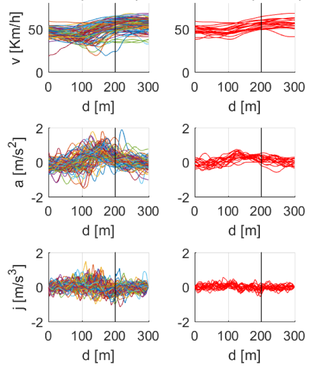
The stretch of road we used for our experiments is shown in Fig.1 and the corresponding data that were collected are in Fig.2.

We used the distance between the the road junction point and the car position as state variable ( $\mathbf{x}_{k}=d(t_{k})$ ) and the car longitudinal speed as control variable ( $\mathbf{u}_{k}=v(t_{k})$ ). From the dataset, we extracted the $20$ trips with the lowest jerk (in red in Fig. 2). We used this reduced dataset as desired behavior for the car. Given this set-up, we were able to compute both $f(\mathbf{d}^{n})$ and $g(\mathbf{d}_{e}^{n})$ from the complete dataset of $100$ trips and the reduced dataset of $20$ trips respectively. These pdfs are shown in Fig. 3, together with the corresponding control pdf (rightward panel).We also note here that $\text{S}(f(\mathbf{d}^{n}))\subseteq\text{S}(g(\mathbf{d}_{e}^{n}))$ and this guarantees the absolute continuity of $f(\mathbf{d}^{n})$ with respect to $g(\mathbf{d}_{e}^{n})$ .

Finally, we decided to constraint the variance of the acceleration (the control variable) and solved the resulting Problem 1 via Algorithm 1. In particular, to make the problem computationally efficient, we approximated all the above pdfs as Gaussian distributions via the Maximum Entropy Principle. Once this was done, we were able to control the closed loop pdf of the system so that it became as close as possible to $g(\mathbf{d}_{e}^{n})$ , given the constraint on the variance - see Figure 4. In the figure, the initial condition was $x_{0}=18$ meters (physically, this is a traffic light outside the UCD gate). Also, the equality constraint was set to have a variance of the closed-loop system higher than the variance of $g(\mathbf{d}_{e}^{n})$ - this is why the closed-loop pdf is flatter.

7 Conclusions

We presented an approach to the synthesis of policies from examples. The key technical novelty of the results is the inclusion of actuation constraints in the problem formulation. This in turn yields policies that can be exported to different systems having different actuation capabilities. After presenting the main results we introduced an algorithmic procedure (code is available upon request). If accepted, the presentation will include a sketch of the proofs and a full report of our experimental results, which could not be included here due to space constraints.

Appendix A Sketch of the proofs

Proof of Property 1

To prove this result we start from the definition of KL-divergence. In particular:

\begin{array}[]{ll}\mathcal{D}_{\text{KL}}\left(\phi\left(\mathbf{y},\mathbf{z}\right)||g\left(\mathbf{y},\mathbf{z}\right)\right):=\\ \quad=\int\int\phi\left(\mathbf{y},\mathbf{z}\right)\left[\ln\frac{\phi\left(\mathbf{y},\mathbf{z}\right)}{g\left(\mathbf{y},\mathbf{z}\right)}\right]\,d\mathbf{y}\,d\mathbf{z}=\\ \quad=\int\int\phi\left(\mathbf{z}|\mathbf{y}\right)\,\phi\left(\mathbf{y}\right)\left[\ln\frac{\phi\left(\mathbf{z}|\mathbf{y}\right)\phi\left(\mathbf{y}\right)}{g\left(\mathbf{z}|\mathbf{y}\right)\,g\left(\mathbf{y}\right)}\right]\,d\mathbf{y}\,d\mathbf{z}=\\ \quad=\underbrace{\int\int\phi\left(\mathbf{z}|\mathbf{y}\right)\left[\phi\left(\mathbf{y}\right)\ln\frac{\phi\left(\mathbf{y}\right)}{g\left(\mathbf{y}\right)}\right]\,d\mathbf{y}\,d\mathbf{z}}_{(1)}\;+\\ \qquad+\underbrace{\int\int\phi\left(\mathbf{y}\right)\left[\phi\left(\mathbf{z}|\mathbf{y}\right)\ln\frac{\phi\left(\mathbf{z}|\mathbf{y}\right)}{g\left(\mathbf{z}|\mathbf{y}\right)}\right]\,d\mathbf{z}\,d\mathbf{y}}_{(2)}.\end{array}

For the term $(1)$ in the above expression we may continue as follows:

\begin{array}[]{ll}&\int\int\phi\left(\mathbf{z}|\mathbf{y}\right)\left[\phi\left(\mathbf{y}\right)\ln\frac{\phi\left(\mathbf{y}\right)}{g\left(\mathbf{y}\right)}\right]\,d\mathbf{y}\,d\mathbf{z}=\\ &=\int\phi\left(\mathbf{z}|\mathbf{y}\right)\,d\mathbf{z}*\left[\int\phi\left(\mathbf{y}\right)\ln\frac{\phi\left(\mathbf{y}\right)}{g\left(\mathbf{y}\right)}d\mathbf{y}\right]\,=\\ &=\mathcal{D}_{\text{KL}}\left(\phi\left(\mathbf{y}\right)||g\left(\mathbf{y}\right)\right)\end{array}

where we used Fubini’s theorem, the fact that that the term on the first line in square brackets is indepedent on $\mathbf{Z}$ and the fact that $\int\phi\left(\mathbf{z}|\mathbf{y}\right)\,d\mathbf{z}=1$ .

By using again Fubini’s theorem, for the term $(2)$ instead we have:

\begin{array}[]{ll}&\int\int\phi\left(\mathbf{y}\right)\left[\phi\left(\mathbf{z}|\mathbf{y}\right)\ln\frac{\phi\left(\mathbf{z}|\mathbf{y}\right)}{g\left(\mathbf{z}|\mathbf{y}\right)}\right]\,d\mathbf{z}\,d\mathbf{y}=\\ &=\int\phi\left(\mathbf{y}\right)\left[\int\phi\left(\mathbf{z}|\mathbf{y}\right)\ln\frac{\phi\left(\mathbf{z}|\mathbf{y}\right)}{g\left(\mathbf{z}|\mathbf{y}\right)}\,d\mathbf{z}\right]\,d\mathbf{y}=\\ &=\int\phi\left(\mathbf{y}\right)\left[\mathcal{D}_{\text{KL}}\left(\phi\left(\mathbf{z}|\mathbf{y}\right)||g\left(\mathbf{z}|\mathbf{y}\right)\right)\right]\,d\mathbf{y}=\\ &=\mathbb{E}_{\phi(\mathbf{Y})}\left[\mathcal{D}_{\text{KL}}\left(\phi(\mathbf{z}|\mathbf{Y})||\,g(\mathbf{z}|\mathbf{Y})\right)\right],\end{array}

thus proving the result. ∎

Proof of Lemma 1

We prove the result in two steps. First, we rewrite the cost function $\mathcal{L}(f)$ and consider the corresponding augmented Lagrangian. Then, we make use of the Euler-Lagrange (EL) stationary conditions to find $f^{\ast}_{\mathbf{Z}}(\mathbf{z})$ (in what follows we omit the dependencies of functions and pdfs on the random variable $\mathbf{z}$ whenever this is clear from the context).

As a first step, note that the cost function $\mathcal{L}(f)$ of the constrained optimization problem in (9) can be conveniently re-written as $\mathcal{L}(f)=\int f\left[\ln\left(\frac{f}{g}\right)+\alpha\right]\,d\mathbf{z}$ . Then, the augmented Lagrangian takes the following form:

\begin{split}&\mathcal{L}_{aug}\left(f,\lambda_{0},\boldsymbol{\lambda}\right):=\\ &\int f\;\left[\ln\left(\frac{f}{g}\right)+\alpha\right]\,d\mathbf{z}+\lambda_{0}\left(\int f\;\mathds{1}_{\mathcal{S}\left(\mathbf{Z}\right)}\;d\mathbf{z}-1\right)\\ &+\langle\boldsymbol{\lambda},\int f\;\mathbf{h}\left(\mathbf{z}\right)\;d\mathbf{z}-\mathbf{H}\rangle,\end{split}

where $\lambda_{0}$ and $\boldsymbol{\lambda}:=[\lambda_{1},\ldots,\lambda_{c_{\mathbf{z}}}]^{T}$ are the (non-negative) Lagrange multipliers (LMs) corresponding to the constraints of the optimization problem. In turn, the above expression can be re-written as

\begin{split}&\mathcal{L}_{aug}\left(f,\lambda_{0},\boldsymbol{\lambda}\right)=\int f\;\left[\ln\left(\frac{f}{g}\right)+\alpha+\lambda_{0}+\langle\boldsymbol{\lambda},\mathbf{h}\left(\mathbf{z}\right)\rangle\right]\,d\mathbf{z}\\ &-\lambda_{0}-\langle\boldsymbol{\lambda},\mathbf{H}\rangle\end{split}

(49)

Now, we let

\tilde{\alpha}(\mathbf{z})=\alpha(\mathbf{z})+\lambda_{0}+\langle\boldsymbol{\lambda},\mathbf{h}\left(\mathbf{z}\right)\rangle

(50)

and make use of the EL stationary conditions to find the optimal solution. First, we consider the EL stationary condition with respect to the pdf $f$ . These conditions can be written in terms of the quantity under the integral in (49), i.e. in terms of $l(f):=f\;\left[\ln\left(\frac{f}{g}\right)+\tilde{\alpha}\right]=f\;\left[\ln\left(f\right)-\ln\left(g\right)+\tilde{\alpha}\right]$ . In particular, by imposing the stationary condition we obtain:

\frac{\partial l(f)}{\partial f}=\ln\left(\frac{f}{g}\right)+\tilde{\alpha}+1=0.

(51)

Therefore, it follows that all the optimal solution candidates must be of the form:

f(\mathbf{z})=g(\mathbf{z})e^{-\{1+\tilde{\alpha}(\mathbf{z})\}},

(52)

which, by definition of $\tilde{\alpha}$ , becomes

f(\mathbf{z})=g(\mathbf{z})\frac{e^{-\{\alpha(\mathbf{z})+\langle\boldsymbol{\lambda},\mathbf{h}\left(\mathbf{z}\right)\rangle\}}}{e^{1+\lambda_{0}}}.

(53)

Note that the above candidates are a function of the LMs. These can be computed by applying the EL stationary condition with respect to $\lambda_{0},\lambda_{1},\ldots,\lambda_{c_{\mathbf{z}}}$ . This yields the following set of additional conditions:

\frac{\partial\mathcal{L}_{aug}\left(f,\lambda_{0},\boldsymbol{\lambda}\right)}{\partial\lambda_{i}}=0,\ \ \ i=0,\ldots,c_{\mathbf{z}}.

(54)

That is, (54) imply that the LMs associated to the constraints must satisfy:

\int g(\mathbf{z})\frac{e^{-\{\alpha(\mathbf{z})+\langle\boldsymbol{\lambda},\mathbf{h}\left(\mathbf{z}\right)\rangle\}}}{e^{1+\lambda_{0}}}\tilde{\mathbf{h}}_{i}\left(\mathbf{z}\right)\;d\mathbf{z}=\tilde{\mathbf{H}}_{i}\quad i=0,\dots,c_{\mathbf{z}},

(55)

which was obtained by replacing the expression of the optimal solution candidate (53) in (54).

Now, the above set of equations can be solved via Lemma 2 and here we let $\lambda_{0}^{\ast}$ , $\boldsymbol{\lambda}^{\ast}$ be the resulting values of LMs. By substituting the optimal LMs into the expression of the optimal solution candidates yields:

f^{\ast}:=f^{\ast}(\mathbf{z})=g(\mathbf{z})\frac{e^{-\{\alpha(\mathbf{z})+\langle\boldsymbol{\lambda}^{\ast},\mathbf{h}\left(\mathbf{z}\right)\rangle\}}}{e^{1+\lambda_{0}^{\ast}}}.

The proof is then concluded by noticing that $f^{\ast}(\mathbf{z})$ is indeed the optimal solution since the Lagrangian is convex in $f$ . To show convexity, it suffices to consider the second derivative of $l(f)$ and to observe that this is always positive definite (indeed $\frac{\partial^{2}l}{\partial f^{2}}=\frac{\partial\left(\ln\left(f\right)+\tilde{\alpha}+1\right)}{\partial f}=\frac{1}{f}>0$ ).

Finally, the second part of the result follows from evaluating $\mathcal{L}\left(f^{\ast}\right)$ . Indeed:

\begin{array}[]{rl}\mathcal{L}\left(f^{\ast}\right)&=\int f^{\ast}\left[\ln\frac{ge^{-\{\alpha+\langle\boldsymbol{\lambda}^{\ast},\mathbf{h}\rangle\}}}{e^{1+\lambda_{0}^{\ast}}g}+\alpha\right]\,d\mathbf{z}=\\ &=-\int f^{*}\left(1+\lambda_{0}^{\ast}+\langle\boldsymbol{\lambda}^{\ast},\mathbf{h}\rangle\right)\,d\mathbf{z}=\\ &=-\left(1+\lambda_{0}^{\ast}+\langle\boldsymbol{\lambda}^{\ast},\mathbf{H}\rangle\right),\end{array}

(56)

and this completes the proof.∎

Proof of Lemma 2

We prove this result by showing that: (i) $\mathcal{J}\left(\tilde{\boldsymbol{\theta}}\right)$ is strictly convex; (ii) its minimizer must satisfy the set of equations (13).

The proof of statement (ii) comes directly from the evaluation of the first order stationary condition. Indeed, any optimal candidate, say $\tilde{\boldsymbol{\theta}}^{\ast}$ , must satisfy $\nabla\mathcal{J}\left(\tilde{\boldsymbol{\theta}^{\ast}}\right)=0$ . Now, computing $\nabla\mathcal{J}\left(\tilde{\boldsymbol{\theta}^{\ast}}\right)$ yields

\begin{array}[]{l}\tilde{\mathbf{H}}-\int_{\mathcal{Z}}\hat{f}_{1}\left(\mathbf{z}\right)e^{-\langle\tilde{\boldsymbol{\theta}^{\ast}},\;\tilde{\mathbf{h}}\left(\mathbf{z}\right)\rangle}\tilde{\mathbf{h}}\left(\mathbf{z}\right)\,d\mathbf{z}=\\ \tilde{\mathbf{H}}-\int_{\mathcal{Z}}\hat{f}_{2}\left(\mathbf{z},\tilde{\boldsymbol{\theta}^{\ast}}\right)\tilde{\mathbf{h}}\left(\mathbf{z}\right)\,d\mathbf{z}=\mathbf{0},\\ \end{array}

(57)

where we used the definition of $\hat{f}_{2}$ to obtain the second equality. That is, (57) immediately implies that any candidate minimizer of the optimization problem in (14) must fulfil the set of equations (13).

In order to prove strict convexity (i.e. statement (i)) we compute the Hessian of $\mathcal{J}\left(\tilde{\boldsymbol{\theta}}\right)$ and show that this is strictly positive definite in $\tilde{{\Theta}}$ . Indeed, computing the Hessian yields

\begin{array}[]{l}\left[\nabla^{2}\mathcal{J}\left(\tilde{\boldsymbol{\theta}}\right)\right]=\int_{\mathcal{Z}}\left[\tilde{\mathbf{h}}\left(\mathbf{z}\right)\otimes\tilde{\mathbf{h}}\left(\mathbf{z}\right)\right]\hat{f}_{1}\left(\mathbf{z}\right)e^{-\langle\tilde{\boldsymbol{\theta}},\;\tilde{\mathbf{h}}\left(\mathbf{z}\right)\rangle}\,d\mathbf{z},\end{array}

(58)

where $\otimes$ denotes the external product between tensors. Now, since the equations in (13) are algebraically independent, we have (see Definition 2):

\begin{array}[]{l}\exists S\subset\mathcal{Z}:\forall\tilde{\mathbf{v}}\in\mathbb{R}^{c_{\mathbf{z}}}-\{\mathbf{0}\}\\ \langle\left[\nabla^{2}\mathcal{J}\left(\tilde{\boldsymbol{\theta}}\right)\right]\tilde{\mathbf{v}},\,\tilde{\mathbf{v}}\rangle=\\ \int_{S}\langle\tilde{\mathbf{v}},\,\tilde{\mathbf{h}}\left(\mathbf{z}\right)\left(\mathbf{z}\right)\rangle^{2}\hat{f}_{1}\left(\mathbf{z}\right)e^{-\langle\tilde{\boldsymbol{\theta}},\;\tilde{\mathbf{h}}\left(\mathbf{z}\right)\rangle}\,d\mathbf{z}>0.\\ \end{array}

(59)

This implies that $\tilde{\boldsymbol{\theta}}^{\ast}$ is the unique minimizer of the optimization problem, thus concluding the proof. ∎

References

Argall et al. (2009) Argall, B.D., Chernova, S., Veloso, M., and Browning, B. (2009). A survey of robot learning from demonstration. Robotics and Autonomous Systems, 57(5), 469 – 483. https://doi.org/10.1016/j.robot.2008.10.024.
Bryson (1996) Bryson, A.E. (1996). Optimal control-1950 to 1985. IEEE Control Systems Magazine, 16(3), 26–33.
Englert et al. (2017) Englert, P., Vien, N.A., and Toussaint, M. (2017). Inverse kkt: Learning cost functions of manipulation tasks from demonstrations. The International Journal of Robotics Research, 36(13-14), 1474–1488. 10.1177/0278364917745980.
Griggs et al. (2019) Griggs, W., Ordóñez-Hurtado, R., Russo, G., and Shorten, R. (2019). A vehicle-in-the-loop emulation platform for demonstrating intelligent transportation systems. In Control Strategies for Advanced Driver Assistance Systems and Autonomous Driving Functions, 133–154. Springer.
Guilleminot and Soize (2013) Guilleminot, J. and Soize, C. (2013). On the statistical dependence for the components of random elasticity tensors exhibiting material symmetry properties. Journal of elasticity, 111(2), 109–130.
Hanawal et al. (2019) Hanawal, M., Liu, H., Zhu, H., and Paschalidis, I. (2019). Learning policies for markov decision processes from data. IEEE Transactions on Automatic Control, 64, 2298–2309.
Herzallah (2015) Herzallah, R. (2015). Fully probabilistic control for stochastic nonlinear control systems with input dependent noise. Neural networks, 63, 199–207. 10.1016/j.neunet.2014.12.004.
Kárný (1996) Kárný, M. (1996). Towards fully probabilistic control design. Automatica, 32(12), 1719–1722. 10.1016/s0005-1098(96)80009-4.
Kárný and Guy (2006) Kárný, M. and Guy, T.V. (2006). Fully probabilistic control design. Systems & Control Letters, 55(4), 259–265. 10.1016/j.sysconle.2005.08.001.
Kullback and Leibler (1951) Kullback, S. and Leibler, R. (1951). On information and sufficiency. Annals of Mathematical Statistics, 22, 79–87.
Kárný and Kroupa (2012) Kárný, M. and Kroupa, T. (2012). Axiomatisation of fully probabilistic design. Information Sciences, 186(1), 105 – 113. https://doi.org/10.1016/j.ins.2011.09.018.
Pegueroles and Russo (2019) Pegueroles, B.G. and Russo, G. (2019). On robust stability of fully probabilistic control with respect to data-driven model uncertainties. In 2019 18th European Control Conference (ECC), 2460–2465. 10.23919/ECC.2019.8795901.
Peterka (1981) Peterka, V. (1981). Bayesian approach to system identification. 239–304. 10.1016/b978-0-08-025683-2.50013-2.
Quinn et al. (2016) Quinn, A., Kárnỳ, M., and Guy, T.V. (2016). Fully probabilistic design of hierarchical bayesian models. Information Sciences, 369, 532–547. 10.1016/j.ins.2016.07.035.
Ramachandran and Amir (2007) Ramachandran, D. and Amir, E. (2007). Bayesian inverse reinforcement learning. In Proceedings of the 20th International Joint Conference on Artifical Intelligence, IJCAI’07, 2586–2591. Morgan Kaufmann Publishers Inc., San Francisco, CA, USA.
Ratliff et al. (2006) Ratliff, N.D., Bagnell, J.A., and Zinkevich, M.A. (2006). Maximum margin planning. In Proceedings of the 23rd International Conference on Machine Learning, ICML ’06, 729–736. ACM, New York, NY, USA. 10.1145/1143844.1143936.
Ratliff et al. (2009) Ratliff, N.D., Silver, D., and Bagnell, J.A. (2009). Learning to search: Functional gradient techniques for imitation learning. Autonomous Robots, 27(1), 25–53.
Sutton and Barto (1998) Sutton, R.S. and Barto, A.G. (1998). Introduction to Reinforcement Learning. MIT Press, Cambridge, MA, USA, 1st edition.
Wabersich and Zeilinger (2018) Wabersich, K.P. and Zeilinger, M.N. (2018). Scalable synthesis of safety certificates from data with application to learning-based control. In 2018 European Control Conference (ECC), 1691–1697. 10.23919/ECC.2018.8550288.
Xu and Paschalidis (2019) Xu, T. and Paschalidis, I.C. (2019). Learning models for writing better doctor prescriptions. In 2019 18th European Control Conference (ECC), 2454–2459. 10.23919/ECC.2019.8796280.
Ziebart et al. (2008) Ziebart, B.D., Maas, A., Bagnell, J.A., and Dey, A.K. (2008). Maximum entropy inverse reinforcement learning. In Proc. AAAI, 1433–1438.