Deep learning to discover and predict dynamics on an inertial manifold
Abstract
A data-driven framework is developed to represent chaotic dynamics on an inertial manifold (IM), and applied to solutions of the Kuramoto-Sivashinsky equation. A hybrid method combining linear and nonlinear (neural-network) dimension reduction transforms between coordinates in the full state space and on the IM. Additional neural networks predict time-evolution on the IM. The formalism accounts for translation invariance and energy conservation, and substantially outperforms linear dimension reduction, reproducing very well key dynamic and statistical features of the attractor.
I Introduction
Partial differential equations are formally infinite-dimensional, but the presence of dissipation (through viscosity or diffusion, for example) leads to the expectation that the long-time dynamics collapse onto a finite-dimensional invariant manifold Hopf 1948. Specifically, for some systems, including the Kuramoto-Sivashinsky equation (KSE) that we consider here, it can be proven that all initial conditions exponentially approach an inertial manifold of finite dimension Foias et al. 1988a, on which the long time dynamics evolve. For states on the IM, , one can in principle find a coordinate transformation to coordinates on the inertial manifold, a change of coordinates back to the full space, and a dynamical system on . (Alternately, one could represent the dynamical system in differential form .) This dynamical system is an exact reduced-order model (ROM). Such a model can be practically useful, for computationally efficient simulations of a complex process, and may also be fundamentally important, since the coordinates represent the key dynamical variables for the phenomenon of interest.
In the present work, we use “data” in the form of chaotic solutions to the KSE with periodic boundary conditions, to find neural-network (NN) representations of the functions , and . Many prior studies of inertial manifolds, and approximations thereof, take the inertial manifold to be the graph of a function such that , where is a projection onto the leading eigenfunctions of the linear operator for the PDE Zelik 2013; Foias et al. 1988b; Graham et al. 1993. The present work is not subject to this restriction. Furthermore, our formalism explicitly accounts for the important physical features of translation invariance and energy conservation found in this system, and reproduces, very well, with a minimal number of degrees of freedom, key dynamic and statistical features of the attractor.
A standard machine learning method for nonlinear dimension reduction is the undercomplete autoencoder Hinton and Salakhutdinov 2006; Goodfellow et al. 2016. This is a pair of neural networks, one mapping from a high-dimensional space to a low-dimensional one, and the second doing the reverse. The networks take data as input, compute an output and are trained to minimize a loss function summed over a batch of data vectors . Autoencoders have been used for nonlinear dimension reduction in many applications (Hinton and Salakhutdinov 2006), including turbulent flow fields Omata and Shirayama 2019; Milano and Koumoutsakos 2002. For dynamical systems, autoencoders have been used to explicitly yield coordinate transformations on which the dynamics are linear (Otto and Rowley 2019; Lusch et al. 2018) (e.g. to determine eigenmodes of the Koopman operator) or have a sparse representation (Champion et al. 2019). Gonzalez et al. (Gonzalez and Balajewicz 2018) have combined autoencoders with nonlinear time-evolution models for reconstruction of dynamics of isotropic turbulence and lid-driven cavity flow. Lee and Carlberg (Lee and Carlberg 2019) give an overview of nonlinear model reduction with NNs and application to transient dynamics of Burgers equation. The physical interpretation of NN representations of physical phenomena has been explored in Iten et al. Iten et al. 2020.
Other studies have focused on developing NNs for evolving equations with chaotic dynamics without nonlinear dimension reduction. An early example of this is González-García et al. (González-García et al. 1998), who used a NN to predict the right hand side of the discretized KSE. Specificallly, they input the full state of the KSE and its derivatives into a NN to predict the parameters of a Runge-Kutta method for time integration. More recently larger NN have been used for prediction. For example, Pathak et al. (Pathak et al. 2018) showed that a reservoir network trained with time-evolution “data” from the KSE was capable of making excellent predictions of future time-evolution. No explicit model reduction was performed. In (Lui and Wolf 2019), proper orthogonal decomposition (POD) and a spectral version (SPOD), both linear dimension reduction techniques, were used to reduce the dimension of fluid flow data that were then used to train a NN for time-evolution. Vlachas et al. (Vlachas et al. 2018) combined various linear dimension reduction approaches with a long-short term memory NN and mean stochastic modeling to keep trajectories on the attractor. Similarly, in (Wan et al. 2018) a long-short term memory NN was used in a nonlinear Galerkin approach to estimate the nonlinearity, a task often achieved by assuming lower modes evolve slowly, and iteratively solving for the higher modes (Titi 1990; Foias et al. 1988c; Jolly et al. 1990; Graham et al. 1993; Matthies and Meyer 2003).
Although methods exist for modeling dynamics on an IM, estimating remains a difficult problem. In Kuptsov and Kuptsova 2019, an autoencoder is used to estimate from data for the dynamics of the complex Ginzburg-Landau (CGL) equation; however the dynamics on are not modeled. A dynamical approach to determining was taken in (Yang et al. 2009), where the covariant Lyapunov vectors of trajectories the KSE and the CGL were found to decompose into “physical” and “isolated” modes. Physical modes are entangled, in the sense that tangencies between them result in perturbations of a single mode effecting other modes, whereas isolated modes lack tangencies with physical or isolated modes. This suggests the number of physical modes corresponds to . Expanding on that work, Ding et al. (Ding et al. 2016) found the dimension for the KSE in similar ways using Floquet vectors from an ensemble of unstable periodic orbits that are close to the chaotic attractor. The present work combines data-driven dimension reduction and time evolution using an efficient autoencoder structure that incorporates translation symmetry and energy conservation.
II Formulation
Our testbed for this approach is the KSE,
| (1) |
with periodic boundary conditions in the domain . We select , , and because these domain sizes yield increasingly chaotic dynamics, and is known at Ding et al. 2016. Solutions to this equation are only unique to within a translation that we will represent with a phase variable . This equation has an energy conservation principle: when time-averaged, the energy production rate balances the dissipation rate . Here represents averaging over . These properties are incorporated into the dimension reduction formulation as detailed below. Trajectories of (1) were generated using a Fourier spectral method in space and a fourth-order time integration scheme Kassam and Trefethen 2005 with the code available from Cvitanović et al. Cvitanović et al. 2016. The solution is represented on a uniformly-spaced mesh of points; we denote the solution on this mesh as , so is the dimension of the full state space in the present system.

III Methodology and Results
Figure 1 illustrates our framework for finding the inertial manifold and the dynamical system on it. The first step of the process exploits translation invariance: the solution at every time instant is transformed into a pattern and a phase using an approach called the “method of slices” (Budanur et al. 2015a; Budanur et al. 2015b). Factoring out the phase leads to a more compact representation of the data by eliminating the need of training redundant weights for translated signals. (E.g., the representation will not need to separately represent and all of its translations.) Furthermore, such “symmetry reduction” methods have been found to help elucidate the state space structure in fluid mechanics problems such as pipe flow (Willis et al. 2013).
The method of slices involves taking the discrete Fourier transform of the data in to yield . With the data in Fourier space, the phase of the first Fourier mode is found using Now we can construct a phase-aligned solution so that its first Fourier mode is a pure cosine: Storage of for each time instant allows conversion of back to (i.e. contains both and ). Times when approaches zero require special treatment, as was recognized by Budanur et al. (Budanur et al. 2015a). We use the solution they proposed, which is to stretch time according to . The rescaled time is called “in-slice” time. Given any we can always find , and , so it is always possible to move back and forth between the original and phase-aligned solutions and between real and in-slice time. The data used for training the NNs were solutions separated by “in-slice” time units, which corresponds to time units on average for . Data was gathered after the dynamics had settled onto the attractor.
Given the phase-aligned pattern data , the first machine learning task is to find the manifold , of dimension , on which this data lives, or equivalently the coordinate tranformations and . Because the phase of any given data vector is arbitrary, the phase information is not needed for this step. The coordinates and the phase completely describe the state of the system so the dimension of the attractor in the unreduced state space will be . (For further discussion of invariant manifolds in translation-symmetric systems, see Ref. Budanur et al. 2015b.) Indeed, phase alignment allows more efficient representation of the data, because phase information need not be encoded – it is captured separately as noted above.
To find and , we use a variant of a standard undercomplete autoencoder, shown as the “” branch of architecture shown in Figure 1. This variant uses a NN to represent the difference between the data and its projection onto the basis arising from principal components analysis (PCA) of the data set Strang 2019. PCA is widely used for linear dimension reduction because it yields the projection of dimension that minimizes the mean squared deviation from the original data. Let be a square orthogonal matrix whose columns are the PCA basis vectors, and and the projection onto the first and last such vectors, respectively. The encoding step learns the function such that
| (2) |
This structure is shown inside the blue (upper) box in Figure 1. It must be emphasized that there is no approximation in choosing this representation. Furthermore, need not come from PCA; for example, could be the discrete Fourier transform operator or simply the identity, the latter corresponding to using the solution values on the mesh points.
| Function | Shape | Activation | |
|---|---|---|---|
| Encoder | S:tanh | ||
| Decoder1 | S:linear | ||
| Decoder2 | S:linear | ||
| Evolution | S:S:linear | ||
| Evolution | S:S:S:linear | ||
The decoding step takes the data in the inertial manifold coordinates and transforms it back to the full space, as shown in the yellow (lower) box in Figure 1. Again one can think of learning a difference: the decoder learns a function such that
| (3) |
Taking recovers the original IM formulation, but precludes the representation of curved manifolds that do not have a one-to-one mapping from a linear projection. An example of such a manifold is the Archimedean spiral, whose Cartesian representation is ). The autoencoder architecture used here is able to represent this manifold with .
Finally, inserting Eq. 2 into Eq. 3, solving for , and noting that this can be written , shows that the exact solution satisfies , where contains the first components of . This constraint can be satisfied approximately by adding a penalty term to the autoencoder loss function so it becomes
| (4) |
With this structure, we can in principle achieve an exact representation (within the approximation error of the functions and ) of data on a manifold of dimension for all . In general, the functions and , or more generally and , need not come from NNs. Other approaches to nonlinear dimension reduction and function approximation (e.g. tSNE, diffusion maps, kernel regression (van der Maaten and Hinton 2008; Van Der Maaten et al. 2009)) might be useful as well. The overall structure of our approach would be the same.
Autoencoders of the above structure, which we denote hybrid neural networks (HNN) were trained (i.e. the functions and were determined) using the phase aligned data. At a given value of , twenty HNNs (each initialized with different initial guesses for the weights), with were trained for epochs with an Adam optimizer using Keras Chollet et al. 2015. This process was repeated for a range of . Results are reported for the model with the lowest MSE at each value of .
For comparison we trained three variations on the HNN to evaluate the effect of the linear projection (), the PCA change of basis (), and phase alignment steps. In the first variation, denoted PCANN, we built a NN without the “Trunc” and “Expand” blocks in Fig. 1, which corresponds to using the PCA basis, but using and to learn the whole nonlinear coordinate tranformation rather than just the difference from PCA. The next variation builds upon the previous and removes the “PCA” block in Figure 1, which leaves it in the original basis, so we denote it ONN. Then, the last variation is to remove the phase shift (No Shift). Both the PCANN and the ONN are trained with the loss , while the unsifted variation is trained with . Hyperparameter tuning of the NN architectures was performed manually by varying width, depth, and activation functions. All of these variations used the same architecture, shown in Table 1, for functions and .
Figure 2 shows the mean squared error (MSE) on a separate test dataset for the NN methods described above and PCA for . At low , the HNN, PCANN, and ONN all perform similarly, and in all three cases the MSE drops significantly at . For the case of no shifting, the drop appears at because the continuous translation symmetry has not been factored out. All NNs perform orders of magnitude better than PCA. On continuing to increase , the MSE for the HNN continues to improve while the others stagnate, because the HNN only needs correct coefficients of the less relevant higher PCA modes, while the other methods modify all of them. Notably, the abrupt drop in MSE at coincides with the true dimension of the attractor as found in (Ding et al. 2016). The remaining error for for the HNN is small, at , which follows from the fact that at this dimension an exact coordinate transformation exists, so the remaining error is approximation error.
Having in hand the coordinate representation for points on , we now use NNs to learn the dynamical system (“exact” reduced-order model) on the manifold, corresponding to the “” branch in Figure 1. This approach will be denoted “HNN ROM”. We construct discrete time mappings
| (5) |
where and have the architectures shown in Table 1. We use the symbol instead of to emphasize that the discrete time mappings use in-slice time. We chose , which reproduces trajectories well, by allowing for the signal to change an appreciable amount, but not too much, in one time interval. Setting much smaller or larger results in poor model predictions.
Recall that the energy balance for the KSE requires that the production and dissipation rates and must balance on average. We incorporate this fact in the training of the dynamic models as follows. We compute the projection of the data onto and , as shown in Figure 3. The relation between and is narrowly distributed around the line , with a sharp boundary, and we can find maximum and minimum dissipation rates and associated with a given value of . We then add a penalty for crossing this boundary to the loss function for and , as follows:
| (6) |
where and are calculated from . We selected so the second term contributed the same order of error to the loss as the first term. For each , the best dimension reduction model was chosen, and fifty time-evolution models were trained for 200 epochs. Results are reported for the best models, as determined at a given based on producing low errors in both short and long-time statistics.
To illustrate the performance of this approach, which we denote HNN ROM, on predicting dynamics, we first present short-time tracking results and then long-time statistics. All trajectories are evolved from a given initial condition on the manifold, from which we find and by phase alignment and then set . This initial condition in the manifold coordinates is evolved forward in in-slice time with Eq. 5. For validating the performance of the short-time tracking we need a timescale for comparison. Here we consider the integral timescale , where
is the temporal autocorrelation, and the Lyapunov time Ding et al. 2016. Figure 4 shows the temporal autocorrelation of the data and the HNN ROM at are in good agreement for . Likewise, typical trajectories show close tracking for 30 or more real time units. This comparison appears in Fig. 5, where Fig. 5(a) and 5(c) show the evolution of two initial conditions of test data using the dynamical system found with , and the “exact” results are shown in Fig. 5(c) and 5(d) obtained from solving the KSE. These results indicate predictive capability for time scales longer than or , and thus represent very good performance for prediction of chaotic dynamics.
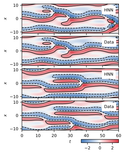
Next, we evaluate the ability of our dynamic model to reproduce key long-time statistical properties of the attractor, focusing on the quantities and that determine the energy production and dissipation in the KSE. We examine predictions both for and for values of either larger or smaller than . The trajectories considered here cover approximately real time units.
Figures 6 and 3, respectively, show the spatial autocorrelation function (averaged over space and time) and the energy balance ( vs. ) of the HNN ROM for and for data, illustrating close agreement of these quantities. These statistics show that long-time trajectories do not diverge from the attractor and that the HNN ROM prediction stays within the envelope of the energy balance, which was the intent of the penalty in the loss for the time-evolution training, Eq. 6. These predictions deteriorate when .
A more detailed representation of the attractor is the joint probability density function (PDF) of the pointwise values of and . Figure 7(a) shows this PDF, on a log scale, as determined from the data. At , the HNN ROM prediction, Fig. 7(b), is very close to the exact PDF. To highlight the effect of the nonlinear autoencoder, we also consider predictions with linear dimension reduction from PCA (i.e. ), and NNs for the dynamics; we denote this approach PCA ROM. At the same dimension, Fig. 7(d) shows that the PCA ROM prediction yields much poorer results. Figure 7(c) shows how the relative difference between the true PDF and the model predictions varies with . For , the predictions are poor for both cases, but for ,the error is small and nearly unchanging for the HNN ROM case, which is unsurprising since . On the other hand, it takes for the PCA ROM to yield a comparable model to the HNN ROM at . This result might be expected based on Whitney’s embedding theorem, which states that any manifold of dimension can be embedded in Guillemin and Pollack 2000.

To investigate the generality of this method, we examine its performance for larger domains, and . For there is one positive Lyapunov exponent (Ding et al. 2016; Edson et al. 2019), whereas the dynamics at and are more chaotic; at these values, Edson et al. (Edson et al. 2019) report four and seven positive Lyapunov exponents, respectively. Data gathering and NN training were performed in the same way as for . Initial trials for the showed poor results, so the capacity of the decoder was increased,as noted in Table 1. Figure 8(a) shows the MSE on a test data set of HNNs with the lowest MSE at various for and . The horizontal axis is centered around the of each domain size inferred from the drop in the MSE. This corresponds to and for and . Increasing dimension still shows a distinct drop in MSE, however it becomes less substantial with increased domain size. The autoencoder performs better has lower MSE than because of the increased capacity.
The results at these domain sizes suggests that there is a linear scaling of with . This observation agrees well with results of Yang et al. (Yang et al. 2009) where they show the number of physical modes (PM) scales linearly with domain size. Figure 8(b) shows (the dimension in the unreduced state space) against the domain size for both our results and their results, along with the extrapolation of their results to smaller domains. The excellent agreement between these results provides additional computational evidence that the dimension of the IM for the KSE scales linearly with .

Finally, we show the attractor recreation with the joint PDFs of and . Figure 9(a) and 9(d) show these for and for trajectories of approximately and real time units, respectively. Model predictions for , Fig. 9(b) and 9(e), and degrees of freedom, Fig. 9(c) and 9(f), are shown for comparison. Unlike with , where models with too few dimensions tended to land on periodic orbits, here, with more degrees of freedom, models with too few dimensions maintain chaos. However, the PDFs for are more diffuse, less accurately recreating the data. In both cases, when the models retain dimensions the joint PDF agrees well with the data, the main discrepancy being a broader tail of the model PDF, i.e. a higher, but still very low, probability of large excursions.
IV Conclusion
We have shown here a framework for data-driven “exact” reduction of a dynamical system onto a low dimensional invariant manifold and time-evolution on that manifold. Translation symmetry and energy conservation, two important features of many systems of interest, are incorporated naturally into the framework. By observing the model reduction error as a function of dimension, the dimension of the invariant manifold can be determined, and once is known, highly accurate model predictions can be obtained. In particular, key statistical quantities in a chaotic system can be well-approximated, indicating that the model dynamics capture the shape of the attractor. In this work, the NNs can be trained on a single processor in a couple days, and time-evolution over time units takes only minutes. At present, it is difficult to predict how network size and training time will scale for more complex problems, especially given that it is not even known in general how scales. Extensions to systems with higher-dimensional dynamics are underway. Systematizing this method could provide a straightforward, data-driven means of approximating the dimension of manifolds and constructing reduced order models, a difficult task for high-dimensional chaotic systems like turbulence.
Acknowledgements.
This work was supported by AFOSR FA9550-18-1-0174 and ONR N00014-18-1-2865 (Vannevar Bush Faculty Fellowship). Code is available at https://github.com/alinot5/KSNN.git.References
- Hopf (1948) E. Hopf, Communications on Pure and Applied Mathematics 1, 303 (1948).
- Foias et al. (1988a) C. Foias, B. Nicolaenko, G. R. Sell, and R. Temam, J. Math. Pure Appl. 67, 197 (1988a).
- Zelik (2013) S. Zelik, Proceedings of the Royal Society of Edinburgh Section A: Mathematics 144, 1245 (2013), arXiv:1303.4457 .
- Foias et al. (1988b) C. Foias, G. R. Sell, and R. Temam, Journal of Differential Equations 73, 309 (1988b).
- Graham et al. (1993) M. D. Graham, P. H. Steen, and E. S. Titi, J Nonlinear Sci 3, 153 (1993).
- Hinton and Salakhutdinov (2006) G. E. Hinton and R. R. Salakhutdinov, Science 313, 504 (2006).
- Goodfellow et al. (2016) I. Goodfellow, Y. Bengio, and A. Courville, Deep Learning (MIT Press, 2016) http://www.deeplearningbook.org.
- Omata and Shirayama (2019) N. Omata and S. Shirayama, AIP Advances 9, 015006 (2019).
- Milano and Koumoutsakos (2002) M. Milano and P. Koumoutsakos, Journal of Computational Physics 182, 1 (2002).
- Otto and Rowley (2019) S. E. Otto and C. W. Rowley, SIAM Journal on Applied Dynamical Systems 18, 558 (2019).
- Lusch et al. (2018) B. Lusch, J. N. Kutz, and S. L. Brunton, Nat Comms 9, 851 (2018).
- Champion et al. (2019) K. Champion, B. Lusch, J. N. Kutz, and S. L. Brunton, ArXiv (2019), 1904.02107v2 .
- Gonzalez and Balajewicz (2018) F. J. Gonzalez and M. Balajewicz, ArXiv (2018), 1808.01346v2 .
- Lee and Carlberg (2019) K. Lee and K. T. Carlberg, Journal of Computational Physics , 108973 (2019).
- Iten et al. (2020) R. Iten, T. Metger, H. Wilming, L. del Rio, and R. Renner, Physical Review Letters 124, 10508 (2020), arXiv:1807.10300 .
- González-García et al. (1998) R. González-García, R. Rico-Martínez, and I. G. Kevrekidis, Computers and Chemical Engineering 22, 10.1016/s0098-1354(98)00191-4 (1998).
- Pathak et al. (2018) J. Pathak, B. Hunt, M. Girvan, Z. Lu, and E. Ott, Phys. Rev. Lett. 120, 024102 (2018).
- Lui and Wolf (2019) H. F. Lui and W. R. Wolf, Journal of Fluid Mechanics 872, 963 (2019).
- Vlachas et al. (2018) P. R. Vlachas, W. Byeon, Z. Y. Wan, T. P. Sapsis, and P. Koumoutsakos, Proceedings of the Royal Society A: Mathematical, Physical and Engineering Sciences 474, 20170844 (2018).
- Wan et al. (2018) Z. Y. Wan, P. Vlachas, P. Koumoutsakos, and T. Sapsis, PLoS ONE 13, e0197704 (2018).
- Titi (1990) E. S. Titi, Journal of Mathematical Analysis and Applications 149, 540 (1990).
- Foias et al. (1988c) C. Foias, M. S. Jolly, I. G. Kevrekidis, G. R. Sell, and E. S. Titi, Physics Letters A 131, 433 (1988c).
- Jolly et al. (1990) M. S. Jolly, I. G. Kevrekidis, and E. S. Titi, Physica D: Nonlinear Phenomena 44 (1990).
- Matthies and Meyer (2003) H. G. Matthies and M. Meyer, Computers and Structures 81, 1277 (2003).
- Kuptsov and Kuptsova (2019) P. V. Kuptsov and A. V. Kuptsova, in Saratov Fall Meeting 2018: Computations and Data Analysis: from Nanoscale Tools to Brain Functions, edited by D. E. Postnov (SPIE, 2019).
- Yang et al. (2009) H. L. Yang, K. A. Takeuchi, F. Ginelli, H. Chaté, and G. Radons, Phys. Rev. Lett. 102, 074102 (2009).
- Ding et al. (2016) X. Ding, H. Chaté, P. Cvitanović, E. Siminos, and K. A. Takeuchi, Phys. Rev. Lett. 117, 024101 (2016).
- Kassam and Trefethen (2005) A.-K. Kassam and L. N. Trefethen, SIAM Journal on Scientific Computing 26, 1214 (2005).
- Cvitanović et al. (2016) P. Cvitanović, R. Artuso, R. Mainieri, G. Tanner, and G. Vattay, Chaos: Classical and Quantum (Niels Bohr Inst., Copenhagen, 2016).
- Budanur et al. (2015a) N. B. Budanur, D. Borrero-Echeverry, and P. Cvitanović, Chaos 25, 10.1063/1.4923742 (2015a).
- Budanur et al. (2015b) N. B. Budanur, P. Cvitanović, R. L. Davidchack, and E. Siminos, Phys. Rev. Lett. 114, 084102 (2015b).
- Willis et al. (2013) A. P. Willis, P. Cvitanović, and M. Avila, Journal of Fluid Mechanics 721, 514 (2013), arXiv:arXiv:1203.3701v1 .
- Strang (2019) G. Strang, Linear algebra and learning from data (Wellesley-Cambridge Press, 2019).
- van der Maaten and Hinton (2008) L. van der Maaten and G. Hinton, Journal of Machine Learning Research 9, 2579 (2008).
- Van Der Maaten et al. (2009) L. Van Der Maaten, E. Postma, and J. Van den Herik, J Mach Learn Res 10, 66 (2009).
- Chollet et al. (2015) F. Chollet et al., Keras, https://keras.io (2015).
- Guillemin and Pollack (2000) V. Guillemin and A. Pollack, Differential Topology (AMS Chelsea Publishing, Providence, Rhode Island, 2000).
- Edson et al. (2019) R. A. Edson, J. E. Bunder, T. W. Mattner, and A. J. Roberts, ANZIAM Journal 61, 270 (2019), arXiv:1902.09651 .