On QCD strings beyond non-interacting modelPreprint: AIP/123-QED
Abstract
We investigate the implications of Nambu-Goto (NG), Lüscher-Weisz (LW) and Polyakov-Kleinert (PK) string actions for the Casimir energy of the QCD flux-tube at one and two loop order at finite temperature. We perform our numerical study on the 4-dim pure SU(3) Yang-Mills lattice gauge theory at finite temperature and coupling . The static quark-antiquark potential is calculated using link-integrated Polyakov loop correlators. At a high temperature-close to the critical point- We find that the rigidity and self-interactions effects of the QCD string to become detectable. The remarkable feature of this model is that it retrieves a correct dependency of the renormalized string tension on the temperature. Good fit to static potential data at source separations fm is obtained when including additional two-boundary terms of (LW) action. On the other-hand, at a lower temperature-near the QCD plateau- We detect signatures of two boundary terms of the Lüscher-Weisz (LW) string action. The (LW) string with boundary action is yielding a static potential which is in a good agreement with the lattice Monte-Carlo data, however, for color source separation as short as fm.
Keywords:
QCD Phemenonlogy, Effective bosonic string, Nambu-Goto action, Polyakov-Kleinert action, Montecarlo methods, Lattice Guage Theorypacs
12.38.Gc, 12.38.Lg, 12.38.AwI Introduction
The formulation of a string theory for hadrons has been an attractive proposal since the phenomenological success in explaining Venziano formula Veneziano 1968 even before the formulation of quantum chromodynamics (QCD). Despite the difficulties encountered in the quantization scheme in a fundamental string theory, the proposal to describe the long-distance dynamics of strong interactions inside the hadrons by a low energy effective string Luscher et al. 1980; Luscher and Weisz 2002 has remained an alluring conjecture.
String formation Fukugita and Niuya 1983; Cea and Cosmai 1994; Cea et al. 2016; Flower and Otto 1985; Otto and Stack 1984; Ambjørn et al. 1984; Bali and Schlichter 1996; Wosiek and Haymaker 1987; Sommer 1987; etd; Giacomo et al. 1990; Bali et al. 1995a is realized in many strongly correlated systems and is not an exclusive property of the QCD color tubes Thuneberg 1987; Alford and Good 2008; Kasamatsu and Tsubota 2007; Nielsen and Olesen 1973; Lo and Wright 2005. The normalization group equations imply that the system flows towards a roughening phase where the transverse string oscillations to the classical world sheet effects becomes measurable and can be verified in numerical simulations of lattice gauge theories (LGT).
In the leading Gaussian approximation of the NG action, the quantum fluctuations of the string bring forth a universal quantum correction to the linearly rising potential well known as the Lüscher term in the mesonic configurations. In the baryon a geometrical Lüscher-like terms Jahn and Forcrand 2004; de Forcrand and Jahn 2005 ought to manifest.
The width due to the quantum delocalizations of the string grows logarithmically Luscher et al. 1981 as the two color sources are pulled apart. The character of logarithmic broadening is expected for the baryonic junction Pfeuffer et al. 2009 as well. Precise lattice measurements of the potential in gauge model are in consistency with the Lüscher subleading term for color source separation commencing from distance fm Luscher and Weisz 2002. The effective description is expected to hold over distance scale Caselle and Grinza 2012 where the effects of the intrinsic thickness Vyas 2010 of the flux tube diminish. Many gauge models have unambiguously identified the Lüscher correction to the potential with unprecedential accuracy Juge et al. 2003; Dass and Majumdar 2008; Caselle et al. 2016; Caselle et al. 2003; Pennanen et al. 1997; Brandt and Meineri 2016.
In addition, the string model predictions for the logarithmic broadening Luscher et al. 1981 of the mean-square width of the string at very low temperatures has been observed in several lattice simulations corresponding to the different gauge groups Caselle et al. 1996; Bonati 2011; Hasenbusch et al. 1994; Caselle et al. 2006; Bringoltz and Teper 2008; Athenodorou et al. 2009; Juge et al. 2003; Hari Dass and Majumdar 2006; Giudice et al. 2007; Luscher and Weisz 2004; Pepe 2010; Bicudo et al. 2017
In the high temperature regime of QCD, the overlap of the string’s excited states spectrum would lead to a new quantum state with different characteristics. The free string approximation implies a decrease in the slop of the potential or in other-words a temperature-dependent effective string tension Cardoso and Bicudo 2012; Kaczmarek et al. 2000. The leading-order correction for the mesonic potential turns into a logarithmic term of the Dedekind function which encompasses the Lüscher term as a zero temperature limiting term Luscher and Weisz 2002; Gao 1989; Pisarski and Alvarez 1982. With respect to the string’s width the logarithmic broadening turns into a linear pattern before the deconfinement is reached from below Allais and Caselle 2009; Gliozzi et al. 2010a; Caselle 2010; Gliozzi et al. 2010b.
Nevertheless, this non-interacting model of the bosonic string derived on the basis of the leading order formulation of NG action poorly describes the numerical data in the intermediate distances at high temperatures. For instance, substantial deviations Bakry et al. 2010,hep-lat/1004.0782; Bakry et al. 2012a; Bakry et al. 2011a; Bakry et al. 2012b from the free string behavior have been found for the lattice data corresponding to temperatures very close to the deconfinement point.
The comparison with the lattice Monte-Carlo data supports the validity of the leading-order approximation at source separations larger than fm Bakry et al. 2010,hep-lat/1004.0782; Bakry et al. 2012a; Bakry et al. 2012b for both the potential and the color-tube width profile. The descripancies casts over source separation distances at which the leading-order string model predictions are valid Luscher and Weisz 2002 at zero temperature. In the baryon Bakry et al. 2015; Bakry et al. 2016; Bakry et al. 2011b, taking into account the length of the Y-string between any two quarks, we found a similar behavior Bakry, Ahmed S. et al. 2016.
The fact that the lattice data substantially deviate from the free string description at the intermediate distances and high temperatures has induced many numerical experiments to verify the validity of higher-order model-dependent corrections for the NG action Caselle et al. 2004a; Caselle et al. 2004b before the string breaks Bali et al. 2006.
In the Nambu-Goto (NG) framework it seems that there is no reason to believe that all orders of the power expansion are relevant to the correct behavior of QCD strings Giudice et al. 2009. For example, a first-order term deviating from the universal behavior has been determined unambiguously in 3D percolation model Giudice et al. 2009, no numerical evidence indicating universal features of the corrections beyond the Lüscher term have been encountered among , and confining gauge models Caselle et al. 2004a. Numerical simulations of different gauge models in different dimensions may culminate in describing both the intermediate and long string behavior with different effective strings Caselle et al. 2004a.
However, the modeling of QCD flux-tubes beyond the free string approximation may suggest considering other possiblities such as string’s resistance to bending. These strings with rigid structure ought to exhibit smooth fluctuations Polyakov 1986; Kleinert 1986a. The idea that QCD strings may be rigid appeared long ago and been extensively scrutinized by Kleinert and German.
The perturbative two loop potential at , the exact potential in the large dimension limit Braaten and Tse 1987; Kleinert 1989, the dynamical generation of the string tension Kleinert 1988a have been studied, for example. The theory has other well-founded thermodynamical characteristics such as the partition function Elizalde et al. 1993, free energy and string tension at finite temperature Viswanathan and Zhou 1988a; German 1991; Nesterenko and Pirozhenko 1997 and the deconfinement transition point Kleinert 1987.
In this effective string theory only the smooth flux-sheets over long distance are favored and the sharply creased surfaces are excluded. This implies peculiar geometrical chracteristics that is being controlled via the extrinsic curvature or shape tensor of the surfaces.
The string’s rigidity can intuitively understood in relevance to the vortex line picture of the string which indicates a repulsive Bettencourt and Rivers 1995 nature among the flux tubes. This interpretation seems consisent with flux network within baryon Bakry et al. 2015; Bakry et al. 2016; Bakry et al. 2011b which indicates that the sharply-creased flux sheets are energtically unfavorable. The strings appears aligning itself, either via temperature change or the color sources location, such that the angles between the three flux tubes are equally divided into Bakry et al. 2015; Bakry et al. 2016; Bakry et al. 2011b.
Reviving interests appeared recently to address the rigidity of the QCD flux-tube in the numerical simulations of the confining potential. In fact, both compact gauge group Caselle et al. 2015a; Caselle et al. 2016 and gauge theories in Brandt 2017 has been reported.
The contribution of the boundary action to the open string partition function come into play to recover the symmetry breaking by the cylindrical boundary condition. Two-variant formulas for the Lorentz-invariant boundary corrections to the static potential have been calculated in both the Wilson and the Polyakov-loop correlators cases Caselle et al. 2015a; Aharony and Field 2011; Aharony and Karzbrun 2009; Aharony and Dodelson 2012
These corrections are hoped to reflect some features of the fine structure of the profile of QCD flux-tube Bakry et al. 2018; Bakry et al. 2017a; Brandt 2017; Brandt 2011; Battelli:2019lkz; Dubovsky et al. 2013 at relatively short distances/low temperatures, larger distances/high temperature Juge et al. 2003 or the excited spectrum of the flux-tubes Juge et al. 2003; Bicudo et al. 2018; Juge et al. 1998. Indeed, detectable effects for the boundary corrections to the static quark potential have been shown viable on mitigating the deviations from predictions of the effective string and numerical outcomes Billo et al. 2012a; Caselle et al. 2015a; Brandt 2017. We report similar findings in regard to the width profile of the QCD flux-tube near the critical point ( ) .
One goal of the present paper is to examine the Lorentz-invariant boundary terms in Lüscher-Weisz (LW) effective string action for open string with Dirichlet boundary condition on a cylinder. The analytic estimate laid out for the static potential resulting from two boundary terms at the order of fourth and six derivative could be compatible with the energy fields set up by a static mesonic configurations.
The pure Yang-Mills theory in four dimensions is the closest approximation to full QCD. Even though, we are lacking detailed understanding for the string behavior at high temperature and short distance scale. In this region the deviations from the free string behavior occurs on scales that is relevant to full QCD before the string breaks Bali et al. 2006. The nature of the QCD strings at finite temperatures can be very relevant to many portrayals involving high energy phenomena Caselle et al. 2015b; Giddings 1989 such as mesonic spectroscopy Bali et al. 2013; Kalashnikova 2002; Grach et al. 2008, glueballs Caselle and Pellegrini 2013; Johnson and Teper 2002 and string fireballs Kalaydzhyan and Shuryak 2014, for example. This calls for a discussion of the validity of string effects beyond the free bosonic Nambu-Goto string which is the target of this report.
The map of the paper is as follows: In section(II), we review the most relevant string model to QCD and discuss the lattice data corresponding to the Casimir energy versus different approximation schemes. In section(III), the numerical investigation is focused on the width profile of the energy density and the predictions of the Nambu-Goto (NG) and Polyakov-Kleinert (PK) strings. Concluding remarks and summary are provided in the last section.
II String actions and Casmir energy
The conjecture Yang-Mills (YM) vacuum admits the formation of a very thin string-like object Nambu 1974; Nambu 1979; Luscher et al. 1980 has originated in the context of the linear rise property of the confining potential between color sources. The intuition is in consistency Olesen 1985 with the dual superconductivity Mandelstam 1976; Bali et al. 1996; Di Giacomo et al. 2000a; Di Giacomo et al. 2000b; Carmona et al. 2001; Caselle et al. 2016; Pisarski and Alvarez 1982 property of the QCD vacuum. The color fields are squeezed into a confining thin string dual to the Abrikosov line by the virtue of the dual Meissner effect.
The formation of the string condensate spontaneously breakdown the transnational and rotational symmetries of the YM-vacuum and entails the manifestation of (D-2) massless transverse Goldstone modes in addition to their interactions Goddard et al. 1973; Low and Manohar 2002.
To establish an effective string description, a string action can be constructed from the derivative expansion of collective string co-ordinates satisfying Poincare and parity invariance. One particular form of this action is the Lüscher and Weisz Luscher et al. 1980; Luscher and Weisz 2002, in the physical gauge Dubovsky et al. 2012; Aharony et al. 2012, which encompasses built-in surface/boundary terms to account for the interaction of an open string with boundaries. The Lüscher and Weisz Luscher and Weisz 2004 (LW) effective action up to four-derivative term read
| (1) |
with the physical gauge which restricts the string fluctuations to transverse directions . The vector maps the region into and couplings , are effective low-energy parameters. Invariance under party transform would keep only even number derivative terms.
The open-closed duality Luscher and Weisz 2004 imposes constraint on the kinematically-dependent couplings
| (2) |
which can be shown Billo et al. 2012b; Aharony and Karzbrun 2009 through a nonlinear realization of Lorentz transform is valid in any dimension . The above condition Eq. (2) implies that all the terms with only first derivatives in the effective string action Eq. (1) coincide with the corresponding one of Nambu-Goto action in the derivative expansion. The Nambu-Goto action is the most simple form of string actions proportional to area of the world-sheet
| (3) |
where is the two-dimensional induced metric on the world sheet embedded in the background . On the quantum level the Weyl invariance of the NG action is broken in four dimensions; however, the anomaly is known to vanish at large distances Olesen 1985.
The boundary term describes the interplay between the effective string with the Polyakov loops Luscher and Weisz 2004 at the fixed ends of the string and is given by
| (4) |
where are the couplings of the boundary terms. Consistency with the open-closed string duality Luscher and Weisz 2004 which implies a vanishing value of the first boundary coupling , the leading-order correction due to second boundary terms with the coupling appears at higher order than the four derivative term in the bulk.
An interesting generalization of the Nambu-Goto string Arvis 1983; Alvarez 1981; Olesen 1985 has been proposed by Polyakov Polyakov 1986 and Kleinert Kleinert 1986b to stabilize the NG action in the context of fluid membranes. The Polyakov-Kleinert string is a free bosonic string with additional Poincare-invariant term proportional to the extrinsic curvature of the surface as a next order operator after NG action Kleinert 1986b; Polyakov 1986. That is, the surface representation of the Polyakov-Kleinert (PK) string depends on the geometrical configuration of the embedded sheet in the space-time. The bosonic free string action is equiped with the extrinsic curvature as a next-order operator after NG action Polyakov 1986; Kleinert 1986a.
The model preserves the fundamental properties of QCD of the ultraviolet (UV) freedom and infrared (IR) confinement properties Polyakov 1986; Kleinert 1986a, and is consistent with the formation of the glueballs Kleinert 1988b; Viswanathan and Zhou 1988b, and a real () potential German and Kleinert 1989a; Nesterenko and Shvetz 1992; Ambjorn et al. 2014 with a possible tachyonic free spectrum Kleinert and Chervyakov 1996 above some critical coupling Viswanathan and Zhou 1988b.
The action of the Polyakov-Kleinert (PK) string with the extrinsic curvature term reads
| (5) |
with defined as
| (6) |
The extrinsic curvature is defined as
| (7) |
where is Laplace operator and is the rigidity parameter. The term satisfies the Poincare and the parity symmetries and can also be considered Caselle et al. 2015a in the general class of (LW) actions (1).
The perturbative expansion German and Kleinert 1989a of the rigidity term Eq. (6) reads
| (8) |
has the leading term is given by
| (9) |
The rigidity parameter is tuned so as to weigh favorably the smooth surface configuration over the creased worldsheets. In non-abelian gauge theories this ratio is expected to remain constant in the continuum limit Caselle et al. 2015a.
In the following, prior to drawing a comparison between the numerical Yang-mills lattice data and the various models of the Casimir energy, we review the corresponding confining potential due to each string action in the remaining of this section.
The Casimir energy is extracted from the string partition function as
| (10) |
The partition function of the NG model in the physical gauge is a functional integrals over all the world sheet configurations swept by the string
| (11) |
For a periodic boundary condition along the time direction such that
| (12) |
with an extent equals to the inverse of the temperature and Dirichlet boundary condition at the sources position given by
| (13) |
the eigenfunctions are given by
| (14) |
and eigenvalues of are given by
| (15) |
The determinant of the Laplacian after function regularization Dietz and Filk 1983 reads
| (16) |
where and is the modular parameter of the cylinder. The path integral Eq. (11) and Eq. (10) yields the static potential for the leading order contribution of the NG action . The partition function and the static potential are respectively given by
| (17) |
| (18) |
where is a UV-cutoff and is the Dedekind function defined on the real axis as
| (19) |
The second term on the right hand side encompasses the Lüscher term of the interquark potential. This term signifies a universal quantum effect which is a characteristic of the CFT in the infrared free-string limit and is independent of the interaction terms of the corresponding effective theory. One can extract the string tension dependency on temperature from the slop of the linear terms in . Considering the modular transform of the Eq. (18) and taking the limit of long string, the renormalized string tension to leading order is given by
| (20) |
Deitz and Filk Dietz and Filk 1983 extracted the next to leading order term Polchinski and Strominger 1991 of the Casimir potential from the explicit calculation of the two-loop approximation using the regularization scheme. The static potential of NG string at second loop order Eq. (3) is given by
| (21) |
with and are the second and forth-order Eisenstein series defined as
| (22) | |||||
respectively. With the modular transform of Eq. (21) and considering the limit of long string, the string tension, which defines the slop of the leading linear term of the potential, as a function of the temperature reads
| (24) |
where denotes the string tension of the string at zero temperature. The coefficient of the next higher-order terms can be induced Arvis 1983; Giudice et al. 2009 from the expansion of NG action and leads to the exact NG string tension given by
| (25) |
The boundary term in Lüscher-Weisz action due to the symmetry breaking by the cylindrical boundary conditions by the Polyakov lines. In Refs. Aharony and Field 2011; Billo et al. 2012b the first and second nonvanishing Lorentz-Invariant boundary terms contribution to the potential have been calculated. The modification to the potential received when considering Dirichlet boundary condition are given by
| (26) |
The contribution to the partition function coming from the action
| (27) |
Expanding around the free action yields
| (28) |
The Lorentzian-Invariance imply , the next two non-vanishing Lorentzian-Invariant terms come at order four and six derivative terms at coupling
| (29) |
and coupling
| (30) |
respectively.
The spectral Green function corresponding to solution of Laplace equation with Dirichelet boundary conditions on cylinder
| (31) |
The correlator , which is the line integral over each of the Polyakov loops
| (32) |
becomes after substituting the spectral Green function Eq. (31),
| (33) |
Making use of the function regularization of the series sum
| (34) |
The correlator Eq. (33) yields the following correction to the static potential from the boundary term at coupling ,
| (35) |
The modular transforms of Eq.(26) and Eq.(35) do not yield a linear term proportional to which changes the slop of the potential.
The static potential for smooth open strings was evaluated in German and Kleinert 1989a; German 1991; Braaten and Tse 1987; Nesterenko and Shvets 1992. Employing function regularization Elizalde et al. 1993 the finite-temperature contribution is calculated in Ref. Viswanathan and Zhou 1988a without subtraction Nesterenko and Pirozhenko 1997 to the first loop. Here we show in more detail the calculation of the determinant of the Laplacian to unambiguously show the formulation of the static potential and link between different forms used in the literature.
The partition functions due to the leading order contribution from NG action and rigidity terms
| (36) |
are given by
| (37) |
With the use of the transformation
| (38) |
the partition function can be decoupled into the leading-order NG partition function Eq. (16) multiplied by the corresponding rigidity contribution which appears as the Jacobian of the transformation
| (39) |
and
| (40) |
The eigenvalues of the trace of the triangle operators can be calculated from the eigenvalue equations corresponding to periodic and Dirichlet boundary condition defined as
| (41) |
The eigen functions and eigenvalues are given by
| (42) |
and
| (43) |
respectively. The traces then read
| (44) |
where is an auxilary parameter. In the following we illustrate the function regularization scheme used for the evaluation of the two summations appearing in the above integral.
The sum over is the Epstein-Hurwitz function Viswanathan and Xiaoan 1988. Using Sommerfeld-Watson transform Polchinski 1986 the summation over in the last expression can be presented as a contor integral in the complex plane as
| (45) |
Solving the above integral with the contor to yields the two terms
| (46) |
The second sum over is also the Epstein-Hurwitz function. However, we proceed in the regularization using different integral representation Nesterenko and Pirozhenko 1997 to bring the final closed form in terms of the standard mathematical functions. Each term in this sum can be transformed into the integral presentation corresponding to Euler-Gamma function Lambiase and Nesterenko 1996.
For general the Epstein-Hurwitz function reads
| (47) |
then with the modular transform of of the Jacobi , appearing in the above sum, the zeta function turns into the integral presentation
| (48) |
The integral in the last term can be presented in terms of sum over the modified Bessel functions Pearce 1949 of the second kind . Employing Eq. (47) in Eq. (48) in the partition function Eq. (48) the resultant expression would read
| (49) |
The potential corresponding to the total partion function is thus
| (50) |
The massless limit corresponding to in the above equation yields the doublet degeneracy of the free bosonic string modes or the well-known doubling of Lüscher term in the zero temperature limit,
| (51) |
Let us define a string model for the quark-antiquark potential with the leading extrinsic curvature term in conjunction with two subsequent orders of the NG perturbative expansion corresponding to the free and the leading self-interacting components
| (52) |
The potential of the rigid string with the next to leading order NG contribution is
| (53) |
The string tension form this model can be calculated from the power expansion of in the large limit and it turns out to be
| (54) |
In the limit of high and low temperatures the series sum in Eq. (54) takes the asymptotic forms
| (55) |
and
| (56) |
At short distances, renormalization corrections to the zero temperature string tension have to be taken into account German and Kleinert 1989a; German 1991. The lattice spacing, however, naturally introduces cutoff-scale which affects the value of the returned fit parameters over large source separation distances.
The free NG string is known to reproduce Luscher and Weisz 2002 the subleading aspects of the QCD string over long distances but low temperatures. The increase in the temperature may result in the onset of the string self-interactions at all distance scales. Moreover, other potential aspects of the confining strings may come into play. These include the geometrical constraints on the string fluctuations which reflects on its rigidity/stiffness structure; or in otherwords, its resistance to transverse bending and the role of the Lorentzian-invariant Aharony and Field 2011; Billo et al. 2012b boundary terms at short distances in particular. Considering such models Caselle et al. 2015a, from the pure formal point of view, would introduce corrections to the static potential on both the linearly rising part in addition to the inverse higher powers in the source separation . The rigidity effects may not be dominant but can not be neglected when discussing static potential of spectrum of excited states Juge et al. 2003.
In the following, we numerically measure the two point Polyakov-loop correlators and explore to what extent each of the above string actions can be a sufficiently good description for the potential between the two static color sources.
III Lattice potential and string phenomenology
| 1 | -5.9003 | 0.000246 | ||
|---|---|---|---|---|
| 2 | -4.7622 | 0.000313 | ||
| 3 | -3.7976 | 0.000499 | ||
| 4 | -3.1342 | 0.000657 | ||
| 5 | -2.5985 | 0.000713 | ||
| 6 | -2.1313 | 0.000725 | ||
| 7 | -1.7064 | 0.000758 | ||
| 8 | -1.3134 | 0.000766 | ||
| 9 | -0.9475 | 0.000772 | ||
| 10 | -0.6092 | 0.000827 | ||
| 11 | -0.2932 | 0.000857 | ||
| 12 | 0.0000 | 0.000899 |
III.1 Simulation setup
At fixed temperature , the Polyakov loop correlators address the free energy of a system of two static color charges coupled to a heatbath Polyakov 1978. Within the transfer matrix formalism Luscher and Weisz 2002 the two point Polyakov-loop correlators are the partition function of the string.
The Monte-Carlo evaluation of the temperature dependent quark–antiquark potential at each is calculated through the expectation value of the Polyakov loop correlators
| (57) |
with the Polyakov loop defined as
| (58) |
Making use of the space-time symmetries of the torus, the above correlator is evaluated at each point of the lattice and then averaged. We perform simulations on large enough lattice sizes to gain high statistics in a gauge-independent manner Bali et al. 1995b in addition to reduce correlations across the boundaries. The two lattices employed in this investigation are of a typical spatial size of with a lattice spacing fm.
We choose to perform our analysis with lattices with temporal extents of , and slices at a coupling of value . The two lattices correspond to temperatures just before the deconfinement point, and near the end of QCD plateau Doi et al. 2005.
| Fit | Fit Parameters, | |||
|---|---|---|---|---|
| Interval | ||||
| [2,11] | 0.041865(6) | -0.42355(4) | 111231. | |
| [3,11] | 0.039894(9) | -0.40838(6) | 17494. | |
| [4,11] | 0.03901(1) | -0.4010(1) | 4903.69 | |
| [5,11] | 0.0385(2) | -0.396(2) | 2142.17 | |
| [6,11] | 0.0381(2) | -0.393(2) | 1083.57 | |
| [7,11] | 0.03766(3) | -0.3889(2) | 487.15 | |
| [8,11] | 0.0371(3) | -0.383(3) | 153.693 | |
| [9,11] | 0.0366(6) | -0.378(6) | 19.567 | |
| [2,11] | 0.036250(8) | -0.35054(5) | 627275. | |
| [3,11] | 0.040406(9) | -0.38757(7) | 11136. | |
| [4,11] | 0.04111(1) | -0.3938(1) | 1786.73 | |
| [5,11] | 0.0410(1) | -0.393(1) | 1694.91 | |
| [6,11] | 0.0407(2) | -0.390(2) | 1093.66 | |
| [7,11] | 0.04033(3) | -0.3862(2) | 525.181 | |
| [8,11] | 0.0398(3) | -0.380(4) | 168.203 | |
| [9,11] | 0.0392(6) | -0.374(6) | 21.832 | |
The gauge configurations were generated using the standard Wilson gauge-action employing a pseudo-heatbath algorithm Fabricius and Haan 1984; Kennedy and Pendleton 1985 updating to the corresponding three subgroup elements Cabibbo and Marinari 1982. Each update step/sweep consists of one heatbath and 5 micro-canonical reflections. The gauge configurations are thermalized following 2000 sweeps. The measurements are taken on 500 bins. Each bin consists of 4 measurements separated by 70 sweeps of updates.
The correlator Eq.(60) is evaluated after averaging the time links Parisi et al. 1983 in Eq.(60)
| (59) |
The temporal links are integrated out analytically by evaluating the equivalent contor integral of Eq.(59) as detailed in Ref. de Forcrand and Roiesnel 1985.
The lattice data of the () potential are extracted from the two point Polyakov correlator
| (60) |
III.2 Temperature scale near critical point
Thermal effects become dominant in the SU(3) Yang-Mills model Cardoso and Bicudo 2012; Doi et al. 2005 under scrutiny if the temperature is scaled down close enough to the critical point . The lattice data corresponding to the measured potential Eq. (60) at this temperature are inlisted in Table. 1.
In the following, we consider examining three possible ansatz of the string potential and draw comparisons between their possibly interesting combinations. The target is to understand the relevance of each model at the selected source separation intervals for this temperature scale.
III.2.1 Nambu-Goto string at leading and next-to-leading orders
The potential data are fitted to theoretical formulas of the NG string potential at the leading and next-to-leading orders Eqs. (18) and Eq. (21), respectively. We set the string tension and the renormalization constant as a free fitting parameters. The same value of the string tension taken as a fit parameter as in Ref. Cardoso and Bicudo 2012 and Kaczmarek et al. 2000 is reproduced with the corresponding function of the static potential Gao 1989; Luscher and Weisz 2002 and fit domain.
Table 2 enlists the returned value of the string tension and for various source separations commencing from and fm and extending to fm. The point at fm is excluded from the fits interval due to the overlap of the heatbath plaquettes which is well-known limitation of the link integration method.
The fit of the numerical data to the leading order approximation Eq. (18) produces similar reduction in the residuals by excluding short distance points. The fits return a minimal of at on fm and on fm. However, the values of are outstandingly higher than the corresponding returned values considering the next-to-leading approximation Eq. (21).
Higher-order terms in the free energy provide fine corrections for the value of the returned free-parameter . This parameter is interpreted as the zero temperature string tension, that is, the value that should be returned at zero or low temperature as in Ref. Koma and Koma 2017.
To appreciate the role played by the string tension we disclose the fit behavior of the lattice data at this temperature scale We systematically inspect the returned values of for an interval of selected values of the string tension . The residuals and normalization constant for the corresponding are inlisted in Table. 2 with plots in Fig. 1.
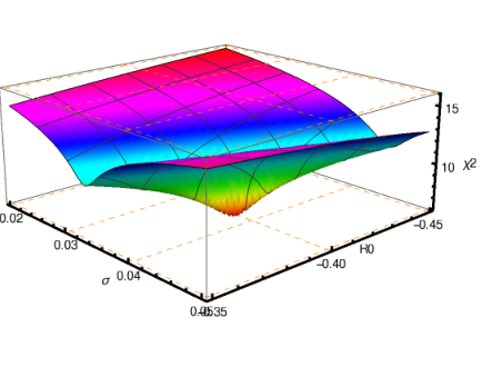
Figure 3-(a) show the stability of the fits and a well-defined global Minimal in the parameter space. The gradual descend of the string tension parameter from 0.045 to 0.041 reduces dramatically the values of (as inlisted in Table 3) till a minimum is reached at for a fit interval from fm. The plot of the static potential owing to the (LO) and the (NLO) of the NG string at three selected values of the string tension is shown in Fig. 1.
The two-dimensional version of Fig 3-(b) depicts how excluding points at short distance, e.g, considering a fit interval , results in a smaller value of with a shifted minimal at as depicted in Fig. 2.
Larger residuals at the (NLO) appear to be stringent at shorter distances fm at string tension value compared to the LO potential ansatz Eq. (21) of the NG string . This suggest that the string’s self-interactions are more relevant to the string configurations swept over long distance scales.
The effective description based only on Nambu-Goto model does not accurately match the potential data. In spite of the fits beyond the free Gaussian approximation, the inclusion of the NLO terms does not provide an acceptable optimization for the potential data. Poor fits persist at both short distance and intermediate distances. The fitted string potential, at its minimal sum of the residuals , produces deviation from the value of the measured value of the zero temperature string tension Koma and Koma 2017.
The fit to the Casimir energy of the self-interacting string returns a value of the zero temperature string tension which deviates at least by of that measured at zero temperature . The pure NG string with its free and next to leading self-interacting pictures does not provide the correct renormalization of the string tension by virtue of the thermal effects.
| Interval | 0.035 | 612.657 | 0.038 | 437.806 | |
| 0.0355 | 292.088 | 0.0385 | 168.529 | ||
| 0.036 | 94.614 | 0.039 | 36.5551 | ||
| 0.0365 | 20.2356 | 0.0395 | 41.4493 | ||
| 0.037 | 68.9527 | 0.04 | 182.793 | ||
| 0.038 | 535.673 | 0.0405 | 460.185 | ||
| 0.0385 | 953.676 | 0.041 | 873.24 | ||
| 0.044 | 13676. | 0.044 | 6180.71 | ||
| 0.045 | 17589.4 | 0.045 | 9019.94 | ||

| Fit | Fit Parameters, =0.9 | ||||
|---|---|---|---|---|---|
| Interval | |||||
| [2,11] | 0.0411327(9) | -0.39693(1) | -0.1746(2) | 2597.5 | |
| [3,11] | 0.04124(1) | -0.39836(1) | -0.202(2) | 2428.1 | |
| [4,11] | 0.04094(2) | -0.3888(4) | 0.20(1) | 1572.9 | |
| [5,11] | 0.0405(2) | -0.35(1) | 2.3(8) | 852.6 | |
| [6,11] | 0.0401(3) | -0.19(7) | 11(4) | 363.1 | |
| [7,11] | 0.03954(5) | 0.47(4) | 52(3) | 99.4 | |
| [8,11] | 0.0389(2) | 2.9(8) | 205(50) | 9.4 | |
| [2,5] | 0.04005(5) | -0.3926(2) | -0.1722(3) | 373.7 | |
| [3,6] | 0.04232(5) | -0.4062(4) | -0.278(4) | 0.049 | |
| [3,7] | 0.0423(4) | -0.4057(3) | -0.274(3) | 2.2 | |
| [3,9] | 0.04189(2) | -0.4032(2) | -0.252(3) | 205.2 | |
| [4,9] | 0.0417(3) | -0.3994(4) | -0.10(2) | 120.5 | |
| [5,10] | 0.04102(3) | -0.368(2) | 1.46(9) | 268.5 | |
| Fit Interval | Fit Parameters, | |||||
|---|---|---|---|---|---|---|
| (LU) | (LU) | (LU) | ||||
| [2,11] | 0.04123(1) | -0.3991(2) | -0.236(5) | 0.023(2) | 2452.4 | |
| [3,11] | 0.04091(2) | -0.332(2) | 2.61(9) | -1.84(6) | 1511.9 | |
| [4,11] | 0.04053(2) | 0.97(5) | 58.1 (2.1) | -44.7(1.6) | 805.8 | |
| [5,11] | 0.0400(3) | 27.7 (12.4) | 1185.4 (520.8) | -948.9 (417.7) | 336.6 | |
| [6,11] | 0.0394(5) | 553.3 (334.4) | 23246.0 (14037.0) | -18790.0 (11352.0) | 89.2 | |
| [2,7] | 0.0423(4) | -0.4090(4) | -0.408(7) | 0.086(3) | 4.8 | |
| [3,8] | 0.04198(4) | -0.393(3) | 0.2(1) | -0.31(8) | 19.4 | |
| [4,9] | 0.04142(4) | 0.12(6) | 22.3 (2.5) | -17.2 (1.9) | 41.3 | |
| Fit Interval | Fit Parameters, | ||||
|---|---|---|---|---|---|
| (LU) | |||||
| (LU) | |||||
| [2,11] | 0.0362498(8) | -0.35054(5) | 0(3.6) | 627275. | |
| [3,11] | 0.040(4) | -0.39(1) | 0(3.7) | 11136 | |
| [4,11] | 0.04245(3) | -0.3756(7) | 0.059(2) | 1148.11 | |
| [5,11] | 0.0435(2) | -0.34(2) | 0.16(5) | 319.657 | |
| [6,11] | 0.0440(2) | -0.30(4) | 0.3(2) | 79.2561 | |
| [7,11] | 0.0442(3) | -0.2(1) | 0.6(7) | 11.592 | |
| [8,11] | 0.044(2) | -0.2(4) | 1(6) | 1.80228 | |
| [2,5] | 0.02677(6) | -0.3095(3) | 0.000291 | 460013. | |
| [3,6] | 0.038(8) | -0.37(2) | 0.002391 | 5774.38 | |
| [3,7] | 0.039(5) | -0.38(2) | 0.002434 | 8395.19 | |
| [4,10] | 0.040(4) | -0.38(1) | 0.002473 | 10933.4 | |
| [4,10] | 0.04214(5) | -0.3879(8) | 0.033753 | 487.035 | |
| [5,10] | 0.04344(4) | -0.360(2) | 0.108(5) | 119.563 | |
| Fit Interval | Fit Parameters, | |||||
|---|---|---|---|---|---|---|
| (LU) | (LU) | |||||
| [2,11] | 4.169(4) | -0.3929(5) | 0.025(1) | -0.199(2) | 2487.2 | |
| [3,11] | 4.343(2) | -0.359(1) | 0.129(3) | -0.533(6) | 501.3 | |
| [4,11] | 4.395(2) | -0.337(2) | 0.244(9) | -1.1(3) | 161.6 | |
| [5,11] | 4.42(2) | -0.32(4) | 0.5(3) | -3(2) | 38.8 | |
| [6,11] | 4.42(8) | -0.353(8) | 1.0(2) | -9(1) | 4.7 | |
| [7,11] | 4.39(4) | -0.48(4) | 3(2.9) | -25(7) | 0.071 | |
| [2,6] | 0.041(1) | -0.39(1) | 0.01(5) | -0.18(7) | 752.6 | |
| [3,7] | 0.0428(2) | -0.400(3) | 0.03(1) | -0.31(3) | 0.74 | |
| [3,9] | 0.04327(4) | -0.385(1) | 0.066(3) | -0.40(1) | 40.9 | |
| [4,10] | 0.04394(3) | -0.355(2) | 0.173(9) | -0.97(4) | 58.9 | |
| [5,10] | 0.04430(3) | -0.343(4) | 0.31(3) | -2.6(2) | 14.7 | |
| Fit Interval | Fit Parameters, | |||||
|---|---|---|---|---|---|---|
| (LU) | (LU) | |||||
| [2,11] | 0.0409(5) | -0.390(2) | 0.01(3) | -0.067(7) | 4460.22 | |
| [3,11] | 0.04327(2) | -0.354(1) | 0.109(2) | -0.323(4) | 558.3 | |
| [4,11] | 0.04393(2) | -0.312(2) | 0.23(8) | -0.89(3) | 154.9 | |
| [5,11] | 0.04422(2) | -0.248(7) | 0.45(3) | -2.6(1) | 36.02 | |
| [6,11] | 0.04415(9) | -0.11(3) | 1.1(2) | -7.9(9) | 4.44 | |
| [2,6] | 0.0409(9) | -0.390(4) | 0.01(6) | -0.06(1) | 3835.6 | |
| [3,8] | 0.0427(1) | -0.391(2) | 0.032(5) | -0.205(9) | 13.5 | |
| [4,10] | 0.0439(4) | -0.335(3) | 0.162(8) | -0.71(3) | 56.3 | |
| [5,10] | 0.0443(3) | -0.284(9) | 0.30(3) | -2.0(2) | 14.0 | |
| Fit Interval | Fit Parameters, | |||||||
|---|---|---|---|---|---|---|---|---|
| (LU) | (LU) | (LU) | ||||||
| [2,11] | 0.043519, 0.0000183 | -0.36374, 0.000937 | -0.140876, 0.0032 | -0.903213, 0.013 | 0.222968, 0.00464167 | 437.185 | ||
| [3,11] | 0.0439943, 0.0000204 | -0.404129, 0.00240 | 0.258954, 0.0100 | -4.24603, 0.188 | 2.25785, 0.120102 | 145.932 | ||
| [4,11] | 0.0442363, 0.0000234 | -1.36259, 0.0873 | 0.502746, 0.038 | -47.2974, 3.9 | 34.353, 3.07522 | 34.16 | ||
| [5,11] | 0.0441876, 0.0000808 | -13.6639, 2.41 | 1.03577, 0.206 | -568.27, 102.6 | 689.797, 82.3587 | 3.96 | ||
| [2,8] | 0.0432653, 0.0000787 | -0.395082, 0.00194 | 0.0545925, 0.00554004 | -0.569233, 0.0288 | 0.123925, 0.00867162 | 5.41 | ||
| [3,8] | 0.0437036, 0.000155 | -0.401344, 0.00342 | -0.0855039, 0.0161917 | -1.42324, 0.399 | 0.628589, 0.23702 | 0.9 | ||
| [3,9] | 0.043877, 0.000071 | -0.401914, 0.0030 | 0.120593, 0.0111493 | -2.10003, 0.285 | 1.02458, 0.173838 | 7.4 | ||
| [4,9] | 0.0442943, 0.000106759 | -0.78807, 0.146409 | 0.198267, 0.0383622 | -19.6914, 6.71211 | 14.3284, 5.07934 | 0.7 | ||
| [4,10] | 0.0443398, 0.0000340 | -1.08879, 0.109 | 0.330004, 0.0378015 | -34.0812, 4.99 | 25.1703, 3.7973 | 12.5 | ||
III.2.2 Boundary terms in Lüscher-Weisz action
Effects such as the interaction of the string with the Ployakov lines at the boundaries may be relevant to the discrepancies in the effective string description at the short and intermediate string length. The contribution to the Casmir energy due to the two next-to-leading nonvanshing term in Lüscher-Weisz action Eq. (1) does not not affect the slop of the linearly rising part of the potential. However, the effects are received as inverse powers in and are given by of Eq (63).
Since the leading nonvanshing boundary terms appear at the order of four derivative term Eq. (4) in Lüscher-Weisz action Eq. 1, It may be more convenient to discuss the corresponding effects (26) in conjunction with the NLO form of the potential of the NG action Eqs. 21 with the renormalization of the string tension included.
For the purpose of the discussion of the numerical data of the static meson potential, We define the following possible combinations of LO and NLO Nambu-Goto static potential with boundary terms,
| (61) | ||||
| (62) | ||||
| (63) |
where subscripted denotes either the LO NG static potential or the NLO Eq. (3). The potential data are fitted to the static potential with a two possibly interesting combinations of the boundary terms and given by Eq. (61) and Eq. (63), respectively. The inspection of each boundary term allows for understanding of the relevance of each boundary parameters to the fit arrangement. The corresponding returned values of and fit parameters are enlisted in Table 4, 8 and 5, considering various fit intervals. The fit to the static potential of the model Eq. (61) returns values for the parameter which appear to vary dramatically with the considered range. The values of are still high when considering the entire fit-interval fm. Even though, none trivial improvements in the values of are retrieved as shown in Table. 4 compared to that obtained by merely considering the NG string potential Eqs. (21) (Table. 3). The fits to the static potential with the boundary term produce acceptable value for shorter fit intervals commencing from fm.
With the interchange of the term in place of in the string model Eq. (61), the fits are not surprisingly good. However, the interesting observation is that the fits at shorter distances commencing from fm upto fm, for both models and , are remarkably good with a returned (Table 5).
Inspection of Tables 4 and 5 indicates that fits to the NLO form of (NG) string with boundary term produce very close value of as the pure NG string . The same observation holds for the fits to and . Acceptable value of are returned over the fit interval fm.
Despite of the reductions in the minima of , the string models with boundary terms have no significantly different behavior with respect to the string tension parameter. This is consistent with the modular transforms where the inverse of the cyliner’s modular parameter does not produce terms linear in . Therof, the boundary corrections to the static potential do not contribute to the renormalization of the string tension.
III.2.3 Rigidity terms in Polyakov-Kleinert action
Establishing a precise string description of the potential data and a correct thermodynamic behavior for the string tension at high temperature have been a long withstanding issues in many investigated gauge models. The consideration of the boundary terms solely does not provide an optimal fits and other possible string properties may be questioned in this context. The possible rigidity/stiffness/self-repulsion of QCD flux tube; or the resistance to sharp transverse-bending should manifest by the onset of the excited fluctuations at high temperatures.
In order to unambiguously appreciate the changes on the fits when the rigidity of the string is taken into account, we discuss the modified static potential of rigid string in conjunction with both the leading and the next-to-leading approximations to NG action and Eqs. (64), separately.
More variants of string models can be attained by including other combinations of the rigid terms such as,
| (64) | ||||
| (65) | ||||
| (66) | ||||
| (67) |
the above compilations are particular choices of terms from the most general formalism Lüscher-Weisz action.
We proceed in the fit analysis of the static potential data without fixing the value of the string tension. The rigidity factor, which weighs the extrinsic curvature tensor, and the ultraviolet cutoff are taken as a free fit parameters as well. Table. 6 summarizes values of obtained from fits to Eq. (64). We remark the following points:
Figure 5 plots the returned values versus both the string tension and rigidity. The plot indicates the quality of the fit in the parameteric space , the oscillatory nature of when the rigidity is included and attainment of the global minima of at .
Drawing comparison between the returned in Table. 2 and Table 6 reveals significant improvement in the fit behavior with the rigidity term of the string model Eq. (64) over the pure NG string potential given by Eq. (18) and (21).
The residuals are reduced on the fit interval fm, the returned indicate good values for fm. Remarkably, the value of the returned string tension on the interval fm and on the interval fm is shifted above the value obtained from considering fits to merely the static potential of the pure NG string. The fit to Eq. (64) results in a value of the string tension which, within the numerical uncertainities, is equivalent to that reproduced at zero temperature measurements Koma and Koma 2017.
The consideration of the two-parameter rigid string model with the next-to-leading order NG potential of Eq. (64) results in a smaller compared to the fit with the two parameter string models of formula Eq. (61). Nevertheless, the fit with boundary action models (Table. 5)compares to the rigid string when considering larger parametric space,i.e., the three parameter model of Eqs. (63).
The plot in Fig. 6(a) is the fit of the static potential of the rigid string for the fit intervals over the given in Table 6. A descending sequence of the values of rigidity parameter are returned. The values of decreases from to as one includes smaller distances into the fit range over intermediate distances to fm.
Large uncertainties in the rigidity parameter are returned from the fits with the decrease of minimal source separation of the fit range . This is perhaps owing to higher-order terms in the perturbative expansion of the extrinsic curvature in the rigid string action.
The renormalization of the string tension has been explicitly given by German German and Kleinert 1989b; German 1991 long ago. The misfortune that we are lacking an ansatz for the potential for the two-loop static quark-antiquark German and Kleinert 1989a; German and Kleinert 1989b; German 1991 at finite temperature scales and dimension. We evaluate the thermodynamic properties of this string gas at two-loop orders and examine the effects on the relatively short distance physics in a separate report Bakry et al. 2017b.
Despite of the outstanding match between the static potential curve with and the data over the range , the plot in Fig. 6(a) exhibits palpable deviations if short distances fm are not included in the fit interval.
Nevertheless, the reduction in the residual from the fits to Eq. (64) and the subsequent retrieve of the correct normalization of the string tension grasp a clue that the rigid properties are nontrivial ingredient in a faithful representation of the physics of the QCD flux-tube.
As discussed above, the boundary corrections to the static potential are mitigating the short distance mismatch with the data; whereas, the rigidity term evidently returns acceptable values of and string tension over long distances. An optimization of both models is expected, thereof, to provide a prospect for an extended distance scale of validity.
The models given by Eq. (65), Eq. (66) and Eq. (67) define selected compilations grasping both aspects of the rigidity and boundary effects. Tables. 9, 8 and 7 enlist the parameters and returned from the fits of the numerical data of the static potential to these models, respectively.
Inspection of the above mentioned tables reveals that the two models given by the interchanging the two boundary terms and in Eq. (65), Eq. (66) are yielding almost comparable values of for each given fit interval.
However, the model encompassing both of the boundary terms Eq. (65) provide the best fit for the targeted distance which is the intermediate distance scale [5,11], . Interestingly, the fit over short distances interval in the second panel of Table. 9 is as well indicating a good for most fit intervals. The plot of the static potential in Figs. 6(a), Fig. 6(b) and Fig. 7 respectively illustrates the subsequent diminish of the errors as the boundary terms are included to rigid model.
The panel of Fig. 8 congregates subfigures each show the variation in the parametric subspace versus the below bound of the fit interval whereas the last point has kept fixed at fm.
The returned zero-temperature string tension unless otherwise the rigidity is considered is decreasing with the increase of lower bound of the fit to achieve acceptable reduction of . The remarkable feature is that the contrary of this behavior is observed when we string models with rigidity are considered.
The rigidity parameter appears to assume stable values in the range fm. At fm, the large uncertainities are suppressed owing to the additional of boundary terms of couplings and .
The optimal is attained at fm for the rigid string model with two boundary terms of Eq. (67). The increase in is almost dramatic for all other models fm. However, good indicating the long distance behavior of effective bosonic strings are obtained from distances and decreases according to a certain selection from the extended parametric space to fm.
III.3 Temperature scale near the Plateau
The analysis of the pure gluonic configuration near the end of QCD plateau is very interesting since a small change in the temperature could produce essential different effects on the properties of the confining force. It ought to be instructive to extend the above reported analysis to the lower temperature scale where the thermal fluctuations are expected to be milder.
In the following we question the string self-interaction and the rigidity together with the boundary terms at each selected source separation intervals. Our target is to illuminate which terms in the interaction potential which persist to provide a good match with the numerical data regardless of the temperature scale in addition to the fit ansatz which nolonger have palpable effects on the fit behavior with the decrease of the temperature.
| 1 | -5.09326 | 0.000697444 | ||
|---|---|---|---|---|
| 2 | -4.75149 | 0.00095430 | ||
| 3 | -4.26808 | 0.00151333 | ||
| 4 | -3.72477 | 0.0025312 | ||
| 5 | -3.17865 | 0.00419748 | ||
| 6 | -2.65406 | 0.0067545 | ||
| 7 | -2.1536 | 0.0106855 | ||
| 8 | -1.67372 | 0.0169562 | ||
| 9 | -1.21469 | 0.0269818 | ||
| 10 | -0.781636 | 0.0424626 | ||
| 11 | -0.378375 | 0.0654182 | ||
| 12 | 0.0 | 0.0986779 |
| Fit | Fit Parameters, | |||
|---|---|---|---|---|
| Interval | ||||
| [2,11] | 0.02520(8) | -0.4000(2) | 21875.7 | |
| [3,11] | 0.0392(1) | -0.4586(5) | 795.844 | |
| [4,11] | 0.0435(2) | -0.482(1) | 18.6047 | |
| [5,11] | 0.045(3) | -0.49(2) | 00 | |
| [3,6] | 0.0373(2) | -0.4523(5) | 399.716 | |
| [3,7] | 0.0381(1) | -0.4553(5) | 566.884 | |
| [3,10] | 0.0391(1) | -0.4583(4) | 779.503 | |
| [4,10] | 0.0435(2) | -0.4816(9) | 18.5844 | |
| Fit | Fit Parameters, | |||
|---|---|---|---|---|
| Interval | ||||
| [2,11] | 0.0240(2) | -0.3208(8) | 340026 | |
| [3,11] | 0.0325(2) | -0.4084(6) | 4609.75 | |
| [4,11] | 0.0422(2) | -0.463(1) | 119.701 | |
| [5,11] | 0.0449(3) | -0.481(2) | 2.60999 | |
| Fit Interval | Fit Parameters, | |||||
|---|---|---|---|---|---|---|
| (LU) | (LU) | (LU) | ||||
| (a) | ||||||
| [2,5] | 0.0400(2) | -0.4689(9) | -0.138(1) | 0.0 | 50.9115 | |
| [2,11] | 0.0422(1) | -0.4767(6) | -0.148(1) | 0.0 | 197.566 | |
| [3,11] | 0.0452(2) | -0.489(1) | -0.607(9) | 0.0 | 5.91231 | |
| (b) | ||||||
| [2,5] | 0.0376637, 0.000209043 | -0.456079, 0.000749928 | 0.0 | -0.0481111,0.000478584 | 107.329 | |
| [3,7] | 0.0444179, 0.000296234 | -0.486774, 0.00141769 | 0.0 | -0.213006, 0.00896163 | 1.93 | |
| [2,11] | 0.040609, 0.000129929 | -0.466179, 0.000499672 | 0.0 | -0.0536944,0.000366839 | 451.37 | |
| [3,11] | 0.0445357, 0.000226426 | -0.487308, 0.00111589 | 0.0 | -0.215779, 0.00766315 | 2.96961 | |
| (c) | ||||||
| [2,11] | 0.0451733, 0.00025135 | -0.496249, 0.00150301 | -0.436979, 0.0205995 | 0.104738, 0.00747759 | 1.37428 | |
| [3,11] | 0.0450192, 0.000425963 | -0.494044, 0.00514882 | -0.327809, 0.24461 | 0.0244465, 0.17942 | 1.17367 | |
| Fit Interval | Fit Parameters, | |||||
|---|---|---|---|---|---|---|
| (LU) | (LU) | (LU) | ||||
| (a) | ||||||
| [2,11] | 0.0393(2) | -0.4521(7) | -0.3189(7) | 0.0 | 1005.75 | |
| [2,5] | 0.0332(3) | -0.427(1) | -0.3077(8) | 0.0 | 259.723 | |
| [3,11] | 0.0452(2) | -0.489(1) | -0.607(9) | 0.0 | 5.91231 | |
| (b) | ||||||
| [2,11] | 0.0357542, 0.000149607 | -0.427408, 0.000648593 | 0.0 | -0.119262, 0.000259866 | 2447.1 | |
| [2,5] | 0.0262228, 0.000337028 | -0.387406, 0.00151795 | 0.0 | -0.115406, 0.000226769 | 688.624 | |
| [3,6] | 0.0429852, 0.00039019 | -0.470346, 0.0019032 | 0.0 | -0.424624, 0.00898908 | 6.57496 | |
| [3,7] | 0.0436562, 0.000301773 | -0.473489, 0.00150711 | 0.0 | -0.436586, 0.00787107 | 13.9662 | |
| [3,11] | 0.0442668, 0.000228102 | -0.476414, 0.00117044 | 0.0 | -0.448646, 0.00685283 | 23.7994 | |
| (c) | ||||||
| [2,11] | 0.0456057, 0.000249587 | -0.495268, 0.0015125 | -0.901874, 0.0186775 | 0.217754, 0.00695054 | 1.91735 | |
| [3,11] | 0.0459421, 0.000418268 | -0.50015, 0.00509954 | -1.14027, 0.238561 | 0.394536, 0.176489 | 0.912238 | |
| Fit Interval | Fit Parameters, | ||||
|---|---|---|---|---|---|
| (LU) | |||||
| (a) | |||||
| [3,11] | 0.0392(1) | -0.4586(4) | 0.000139251 | 795.844;2 | |
| [4,11] | 0.0436(2) | -0.4816(9) | 0.000190263 | 18.6047 | |
| [5,11] | 0.045 | -0.5(2) | 0.747119 | ||
| (b) | |||||
| [3,11] | 0.0326(1) | -0.4085(7) | 0.000334052 | 4609.75 | |
| [4,11] | 0.0422(2) | -0.464(1) | 0.000259934 | 23.94 | |
| [5,11] | 0.0449(1) | -0.481(2) | 0.00349991 | 2.61 | |
| [6,11] | 0.0463(6) | -0.46(6) | 0.138479 | 0.312231 | |
| Fit Interval | Fit Parameters, | |||||||
|---|---|---|---|---|---|---|---|---|
| (LU) | (LU) | |||||||
| 2-11 | 0.0423778, 0.0055167 | -0.476726, 0.0409872 | -0.0175304, 0.56730 | -0.159085, 0.620026 | 0.0 | 188.181; | ||
| 3-11 | 0.0452433, 0.000546988 | -0.489922, 0.0148488 | -0.0415493, 0.0793197 | -0.335264, 0.13425 | 0.0 | 1.12352; | ||
| 2-7 | 0.04(1) | -0.44(9) | 0.0165(1.0) | -0.326 (1.3) | 0.0 | 707.179 | ||
| 2-11 | 0.039(6) | -0.45(4) | 0.0170071 (0.54) | -0.33 (0.6) | 0.0 | 979.948 | ||
| 3-11 | 0.045(6) | -0.48(4) | 0.0192 (0.6) | -0.614308(0.6) | 0.0 | 5.9 | ||
III.3.1 The pure Nambu-Goto action
A large value of is returned for fits of color sources separations commencing from . For separations distance fm the NG string description is showing increasingly significant deviations from the LGT data due to the short distance physics and the one dimensional idealization of NG string. In Refs. Caselle and Grinza 2012; Vyas 2010 the intrinsic thickness of the flux-tube has been discussed.
As Table 11 depicts, Excluding the point fm dramatically decreases the returned value of for both the leading order and the next to leading approximation Eqs.(18) and Eqs. (21), respectively. The returned values of the string tension parameter quickly reaches stability even by the exclusion of further points at short distances fm and fm from the fit range. At this temperature, the string tension settles at a stable value of measured in lattice units.
The measured value of at making use of the fits of LO and NLO approximations are the same within the standard deviation of the measurements. We take this value of the string tension as a reference value for the zero-temperature string tension measured also in Koma and Koma 2017. The numerical data for the potential match both the free leading-order NG string and the NLO self-interacting form of Eq.(18)Eq.(21). Approximately the same difference in the value of the string tension is retrieved for fit domains involving short to large separation distances.
Considering the fit of the same data of potential to the two-loop expression of the NG string Eq. (21), the value of does not apprise mismatches for source separation distances commencing from fm. As shown in Table. 12, for different fit ranges with a fixed end point at fm, the fit return acceptable values of with subtle changes in the free fit parameter . The absence of the mismatch between Eq. (21) and the numerical data at this temperature scale does not rule out the validity at this temperature scale.
This points out to the minor role of the higher order modes at the end of the QCD plateau . The pale out of the thermal effects together with a flat plateau region at this temperature is present as well in the string tension measurements Cardoso and Bicudo 2012 and the more recent Monte-Carlo measurements Koma and Koma 2017 which reproduces the same value of of the zero temperature string tension.
It is worth noting, on the otherhand, that the NLO terms alone esclates the fit on intervals apprising an increase in the values by around 6 times larger. The enclosure of the fourth derivative term of the NLO term in the NG action appears, thereof, neither to alter the poor parameterisation behavior nor to indicate significant changes on the value of the string tension shown in Table. 12.
III.3.2 Boundary terms in Lüscher-Weisz action
The values of returned from the fits to and Eq. (61) are enlisted in Table 14. The consideration of the boundary terms or persist to provide good values over short distance intervals fm. The same observation holds at the other temperature . These are well-known deviations from the free bosonic string over short distance even at zero temperature as well. This may suggest a role to the boundary terms for the deviation from the free non-interacting model over short distances fm.
However, the possible fit ansatz , or at NLO in NG string and , or at leading order does not produce good for any fit interval involving fm. Moreover, the first three fit ansatz involving the string self-interaction seem to escalate the fit over this short distance and temperature. The minimal residuals of the fits over the interval fm is provided by the ansatz which produces .
Figure 10 illustrates the fitted potential curves and the recieved small residuals over short distances as fm when the boundary term included into both LO and NLO NG string potentials. The potential curves are scaled by the square of the separation distance to magnify the long distances fits and the corresponding residuals. The plot exhibits the large value of the residuals and deviations over long distances when the point at fm is included into the fit intervals. These deviations are much less compared to the deviations over the same fit interval considering the pure NG string without boundary terms.
III.3.3 Rigidity terms in Polyakov-Kleinert action
Unlike the relative reduction in the square of the residuals at over all distances, very small values of the rigidity parameter is returned at this temperature . The inclusure of the rigidity terms as well as self-interactions at this temperature do not return any sigficant improvement in the fit behavior at short distances at this temperature scale.
Effects such as the string’s rigidity and self-interactions seem to become noticeable at higher temperatures and energies, the question should be posed here is whether these terms with the returned values at higher temperature are consistent at .
In Table we inlisted the returned values at the intermediate distances fm the self-interactions and rigidity do not escalates the fits. At the temperature and string tension value of , Fig(12-a) shows the two solid curves which are the best fits over intervals and with good values , respectively. The fit parameters are given
| (68) |
III.4 String tension
A discussion concerning the order of the phase transition and the value of the temperature at the critical point would be out of the scope of the present discussion. However, a correct string tension dependancy on the temperature entails that at higher temperature would fall into the same theoretical curve fixed by the plateau value of . This is equivalent to say that that all fits to the potential are returning the same value of measured at zero temperature.
In Fig 12 each theoretical curve is a plot corresponding to the respective order in the NG power expansion. Each of these curves is well defined by the plateau value of and endows the string tension dependency on the temperature. Usually, this envolves a measurement extracted from the lattice data through the slop of the linearly rising potential at low-enough temperature.
The perturbative string tension up to the fourth power in the temperature is layed out through Eq.(20) and Eq.(24). The exact temperature-dependent NG string tension is given by Eq. (25). A probable role of more higher-order terms of the power expansion of NG string action may be discussed in the context of the string tension dependency on the temperature.
At the leading order NG string-tension the lattice data point at produces at the fixed parameter , which fits well into the LO of NG string Eq. (20) curve as depicted in Fig. 12. However, at the temperature the string tension yields a value for the same fixed parameter . This value deviates by from that returned from the fit of LO potential of NG string for fits over the largest interval fm.
These deviations at reduce to at NLO Eq. (24) compared to that retrieved from the fits over the same interval. The data point largly deviates from LO of NG string curve as shown in Fig. 12. Moreover, very small correction are received from the term proportional to the six power in the temperature. At the fourth and sixth order the string tension is and , respectively.
The deviations of the theoretical lines from the plateau value at indicate that all orders in NG action do not provide the correct behavior of the temperature-dependent string tension in the present four-dimensional Yang-Mills model. In addition to that, the boundary corrections Eq. (26) and Eq. (35) do not contribute to the renormalization of the string tension, since the modular transform of the potential does not produce terms linearly proprtional to the string length .
Nevertheless, the extrinsic curvature terms in PK action do redefine the temperature-dependence of the string tension. The corrections to the NG string tension are uniquely determined by the value of the rigidity parameter.
In Tables 6, the enlisted parameters of the rigid string model at show returned average value of for fits over both intervals fm and fm. Similarly, in Table 7 where the rigid string fit ansatz includes boundary correction Eq. (65) a stable value is returned over fm and fm.
The string tension dependency on the temperature in rigid string model is given by the series expansion Eq. 54, with the asymptotic forms given by Eq. (56) and Eq. (55) at low and high temperatures, respectively.
Figure. 13 compares the fourth power NG string tension at next to leading order given by Eq.(24) and the corresponding rigid string-tension given by Eq. (55) versus the temperature for the returned .
The rigid string is showing a more flat region at the end of the plateau region rather than the pure NG string. This observation has been reported in model independent calculations of Ref. Cardoso and Bicudo 2012. For rigidity parameter the string tension at at both temperature scale and . It would be desirable to include more lattice data Cardoso and Bicudo 2012 at lower and higher temperature to well-establish the flatness of QCD transition curve, which we report in the future.
IV Summary and Concluding Remarks
In this work, we compared the static quark-antiquark potential of effective bosonic string model of confinement beyond free Nambu-Goto approximation to the Mont-Carlo lattice data Bakry et al. Lattice 2017. The study mainly targets the color source separation fm to fm, where it is well-known that the free string poorly describe the string tension and quark-antiquark potential in the vicinity of the critical point.
The Nambu-Goto (NG) action at two-loop order have been set into comparison with the corresponding Yang-Mills lattice data in four dimensions. The theoretical predictions laid down by the effects of boundary terms in Lüscher-Weisz (LW) action and extrinsic curvature in Polyakov-Kleinert (PK) action have been also considered.
Both the LO and the NLO approximations of Nambu-Goto string show a good fit behavior for the data corresponding to the potential near the end of the QCD plateau region, namely, at . The fit returns almost the same parameterization behavior with negligible differences for the measured zero temperature string tension . The returned value of this fit paramter is in agreement with the measurements at zero temperature Koma and Koma 2017.
We detect signatures of two boundary terms of the Lüscher-Weisz (LW) string action. The (LW) string with boundary action is yielding a static potential which is in a good agreement with the static potential lattice data as well, however, for color source separation as short as fm.
However, at higher temperature near the deconfinement point the fits to the Nambu-Goto string model considering either LO or NLO approximation poorly describes the lattice data of the static potential data for the fit region span the distances under scrutiny fm.
Nevertheless, the fits show reduction of the residuals for the next-to-leading order approximation of the NG string on each corresponding fit interval. In both LO and NLO of NG string good is attained by the exclusion of the data points at short distances, i.e., fm.
The effective description based only on Nambu-Goto model does not accurately describe the potential data which occur as a deviation from the standard value of the string tension and the static potential data. The fit to the Casimir energy of the self-interacting string returns a value of the zero temperature string tension which deviates by of that measured at and zero temperature. This motivated discussing other effects such as the interaction with the boundaries and stiffness of the flux-tube.
The inclusion of leading boundary term of Lüscher-Weisz action in the approximation scheme reduces the residuals of the at all the considered source separations, however, deviations from the value of the zero temperature string tension do not diminish.
The fit of the static potential considering boundary terms of LW action and contributions from the extrinsic curvature of PK action show a significant improvement compared to that considering merely the ordinary Nambu-Goto string for the intermediate and asymptotic color source separation distances . The fits reproduce an acceptable value of and a zero temperature string tension measured at or at Koma and Koma 2017, thus, indicating a correct temperature dependence of the string tension.
The following enlists intervals over which the optimal value of is returned from the fit of the corresponding string model:
- •
- •
Acknowledgements.
We are thankful to S. Brandt, C. Bonati, M. Casselle, Ph. de Forcrand and T. Filk for their very useful comments. This work has been funded by the Chinese Academy of Sciences President’s International Fellowship Initiative grants No.2015PM062 and No.2016PM043, the Recruitment Program of Foreign Experts, the Polish National Science Centre (NCN) grant 2016/23/B/ST2/00692, NSFC grants (Nos. 11035006, 11175215, 11175220) and the Hundred Talent Program of the Chinese Academy of Sciences (Y101020BR0).References
- Veneziano (1968) G. Veneziano, “Construction of a crossing - symmetric, Regge behaved amplitude for linearly rising trajectories,” Nuovo. Cim. A57, 190–197 (1968).
- Luscher et al. (1980) M. Luscher, K. Symanzik, and P. Weisz, “Anomalies of the free loop wave equation in the WKB approximation,” Nucl. Phys. B173, 365 (1980).
- Luscher and Weisz (2002) Martin Luscher and Peter Weisz, “Quark confinement and the bosonic string,” JHEP 07, 049 (2002), arXiv:hep-lat/0207003 .
- Fukugita and Niuya (1983) M. Fukugita and T. Niuya, “The distribution of chromoelectric flux in su (2) lattice gauge theory,” Physics Letters B 132, 374 – 378 (1983).
- Cea and Cosmai (1994) P. Cea and L. Cosmai, “On The Meissner effect in SU(2) lattice gauge theory,” LATTICE 93: 11th International Symposium on Lattice Field Theory Dallas, Texas, October 12-16, 1993, Nucl. Phys. Proc. Suppl. 34, 219–221 (1994), arXiv:hep-lat/9311023 [hep-lat] .
- Cea et al. (2016) Paolo Cea, Leonardo Cosmai, Francesca Cuteri, and Alessandro Papa, “Flux tubes at finite temperature,” JHEP 06, 033 (2016), arXiv:1511.01783 [hep-lat] .
- Flower and Otto (1985) Jon W. Flower and Steve W. Otto, “The field distribution in su(3) lattice gauge theory,” Physics Letters B 160, 128 – 132 (1985).
- Otto and Stack (1984) Steve W. Otto and John D. Stack, “The SU(3) Heavy Quark Potential with High Statistics,” Phys. Rev. Lett. 52, 2328 (1984).
- Ambjørn et al. (1984) J. Ambjørn, Poul Olesen, and C. Peterson, “Three-dimensional lattice gauge theory and strings,” Nuclear Physics B 244, 262–276 (1984).
- Bali and Schlichter (1996) Gunnar S. Bali and Christoph Schlichter, “The Physics of Strong Quark Binding from Lattice Simulations,” Progress of Theoretical Physics Supplement 122, 67–73 (1996), http://oup.prod.sis.lan/ptps/article-pdf/doi/10.1143/PTPS.122.67/5446003/122-67.pdf .
- Wosiek and Haymaker (1987) J. Wosiek and Richard W. Haymaker, “Space structure of confining strings,” Phys. Rev. D 36, 3297–3300 (1987).
- Sommer (1987) Rainer Sommer, “Chromoflux distribution in lattice qcd,” Nuclear Physics B 291, 673 – 691 (1987).
- (13) “Evidence for flux tubes from cooled qcd configurations,” .
- Giacomo et al. (1990) Adriano Di Giacomo, Michele Maggiore, and Štefan Olejník, “Confinement and chromoelectric flux tubes in lattice qcd,” Nuclear Physics B 347, 441 – 460 (1990).
- Bali et al. (1995a) G. S. Bali, K. Schilling, and C. Schlichter, “Observing long color flux tubes in SU(2) lattice gauge theory,” Phys. Rev. D51, 5165–5198 (1995a), arXiv:hep-lat/9409005 [hep-lat] .
- Thuneberg (1987) E. V. Thuneberg, “Ginzburg-landau theory of vortices in superfluid he-b,” Phys. Rev. B 36, 3583–3597 (1987).
- Alford and Good (2008) Mark G. Alford and Gerald Good, “Flux tubes and the type-i/type-ii transition in a superconductor coupled to a superfluid,” Phys. Rev. B 78, 024510 (2008).
- Kasamatsu and Tsubota (2007) K. Kasamatsu and M. Tsubota, “Quantized vortices in atomic Bose-Einstein condensates,” ArXiv e-prints (2007), arXiv:0709.1042 [cond-mat.other] .
- Nielsen and Olesen (1973) H.B. Nielsen and P. Olesen, “Vortex-line models for dual strings,” Nuclear Physics B 61, 45 – 61 (1973).
- Lo and Wright (2005) Amy S. Lo and Edward L. Wright, “Signatures of cosmic strings in the cosmic microwave background,” (2005), arXiv:astro-ph/0503120 .
- Jahn and Forcrand (2004) Oliver Jahn and Philippe De Forcrand, “Baryons and confining strings,” Nucl. Phys. B - Proc. Suppl. 129-130, 700 – 702 (2004), lattice 2003.
- de Forcrand and Jahn (2005) Ph. de Forcrand and Oliver Jahn, “The baryon static potential from lattice QCD,” Nucl. Phys. A755, 475–480 (2005), arXiv:hep-ph/0502039 .
- Luscher et al. (1981) M. Luscher, G. Munster, and P. Weisz, “How Thick Are Chromoelectric Flux Tubes?” Nucl. Phys. B180, 1–12 (1981).
- Pfeuffer et al. (2009) Melanie Pfeuffer, Gunnar S. Bali, and Marco Panero, “Fluctuations of the baryonic flux-tube junction from effective string theory,” Phys. Rev. D 79, 025022 (2009).
- Caselle and Grinza (2012) Michele Caselle and Paolo Grinza, “On the intrinsic width of the chromoelectric flux tube in finite temperature LGTs,” JHEP 1211, 174 (2012), arXiv:1207.6523 [hep-th] .
- Vyas (2010) Vikram Vyas, “Intrinsic Thickness of QCD Flux-Tubes,” (2010), arXiv:1004.2679 [hep-th] .
- Juge et al. (2003) K. Jimmy Juge, Julius Kuti, and Colin Morningstar, “Fine structure of the QCD string spectrum,” Phys. Rev. Lett. 90, 161601 (2003), arXiv:hep-lat/0207004 [hep-lat] .
- Dass and Majumdar (2008) N.D. Hari Dass and Pushan Majumdar, “Continuum limit of string formation in 3d su(2) lgt,” Phys. Lett. B 658, 273 – 278 (2008).
- Caselle et al. (2016) Michele Caselle, Marco Panero, and Davide Vadacchino, “Width of the flux tube in compact U(1) gauge theory in three dimensions,” JHEP 02, 180 (2016), arXiv:1601.07455 [hep-lat] .
- Caselle et al. (2003) M. Caselle, M. Panero, P. Provero, and M. Hasenbusch, “String effects in Polyakov loop correlators,” Nucl. Phys. Proc. Suppl. 119, 499–501 (2003), arXiv:hep-lat/0210023 .
- Pennanen et al. (1997) P. Pennanen, Anthony M. Green, and Christopher Michael, “Flux-tube structure and beta-functions in SU(2),” Phys. Rev. D56, 3903–3916 (1997), arXiv:hep-lat/9705033 .
- Brandt and Meineri (2016) Bastian B. Brandt and Marco Meineri, “Effective string description of confining flux tubes,” Int. J. Mod. Phys. A31, 1643001 (2016), arXiv:1603.06969 [hep-th] .
- Caselle et al. (1996) M. Caselle, F. Gliozzi, Ulrika Magnea, and S. Vinti, “Width of long colour flux tubes in lattice gauge systems,” Nucl. Phys. B460, 397–412 (1996), arXiv:hep-lat/9510019 .
- Bonati (2011) Claudio Bonati, “Finite temperature effective string corrections in (3+1)D SU(2) lattice gauge theory,” Phys.Lett. B703, 376–378 (2011), arXiv:1106.5920 [hep-lat] .
- Hasenbusch et al. (1994) Martin Hasenbusch, Mihai Marcu, and Klaus Pinn, “High precision renormalization group study of the roughening transition,” Physica A: Statistical Mechanics and its Applications 208, 124 – 161 (1994).
- Caselle et al. (2006) Michele Caselle, Martin Hasenbusch, and Marco Panero, “High precision Monte Carlo simulations of interfaces in the three-dimensional ising model: A Comparison with the Nambu-Goto effective string model,” JHEP 03, 084 (2006), arXiv:hep-lat/0601023 [hep-lat] .
- Bringoltz and Teper (2008) Barak Bringoltz and Michael Teper, “Closed k-strings in SU(N) gauge theories : 2+1 dimensions,” Phys. Lett. B663, 429–437 (2008), arXiv:0802.1490 [hep-lat] .
- Athenodorou et al. (2009) Andreas Athenodorou, Barak Bringoltz, and Michael Teper, “On the spectrum of closed k = 2 flux tubes in D=2+1 SU(N) gauge theories,” JHEP 05, 019 (2009), arXiv:0812.0334 [hep-lat] .
- Hari Dass and Majumdar (2006) N. D. Hari Dass and Pushan Majumdar, “String-like behaviour of 4-D SU(3) Yang-Mills flux tubes,” JHEP 10, 020 (2006), arXiv:hep-lat/0608024 [hep-lat] .
- Giudice et al. (2007) Pietro Giudice, Ferdinando Gliozzi, and Stefano Lottini, “Quantum broadening of k-strings in gauge theories,” JHEP 01, 084 (2007), arXiv:hep-th/0612131 [hep-th] .
- Luscher and Weisz (2004) Martin Luscher and Peter Weisz, “String excitation energies in SU(N) gauge theories beyond the free-string approximation,” JHEP 07, 014 (2004), arXiv:hep-th/0406205 [hep-th] .
- Pepe (2010) M. Pepe, “String effects in Yang-Mills theory,” Proceedings, 28th International Symposium on Lattice field theory (Lattice 2010): Villasimius, Italy, June 14-19, 2010, PoS LATTICE2010, 017 (2010), arXiv:1011.0056 [hep-lat] .
- Bicudo et al. (2017) P. Bicudo, N. Cardoso, and M. Cardoso, “Pure gauge QCD flux tubes and their widths at finite temperature,” (2017), arXiv:1702.03454 [hep-lat] .
- Cardoso and Bicudo (2012) N. Cardoso and P. Bicudo, “Lattice qcd computation of the su(3) string tension critical curve,” Phys. Rev. D 85, 077501 (2012).
- Kaczmarek et al. (2000) Olaf Kaczmarek, Frithjof Karsch, Edwin Laermann, and Martin Lutgemeier, “Heavy quark potentials in quenched qcd at high temperature,” Phys. Rev. D 62, 034021 (2000).
- Gao (1989) Mingshen Gao, “Heavy quark potential at finite temperature from a string picture,” Phys. Rev. D40, 2708 (1989).
- Pisarski and Alvarez (1982) Robert D. Pisarski and Orlando Alvarez, “Strings at finite temperature and deconfinement,” Phys. Rev. D 26, 3735–3737 (1982).
- Allais and Caselle (2009) A. Allais and M. Caselle, “On the linear increase of the flux tube thickness near the deconfinement transition,” JHEP 01, 073 (2009), arXiv:0812.0284 [hep-lat] .
- Gliozzi et al. (2010a) F. Gliozzi, M. Pepe, and U.-J. Wiese, “The Width of the Confining String in Yang-Mills Theory,” Phys.Rev.Lett. 104, 232001 (2010a), arXiv:1002.4888 [hep-lat] .
- Caselle (2010) M. Caselle, “Flux tube delocalization at the deconfinement point,” JHEP 08, 063 (2010), arXiv:1004.3875 [hep-lat] .
- Gliozzi et al. (2010b) F. Gliozzi, M. Pepe, and U. J. Wiese, “Linear broadening of the confining string in Yang-Mills theory at low temperature,” (2010b), arXiv:1010.1373 [hep-lat] .
- Bakry et al. (2010,hep-lat/1004.0782) A. S. Bakry et al., “String effects and the distribution of the glue in static mesons at finite temperature,” Phys. Rev. D 82, 094503 (2010,hep-lat/1004.0782).
- Bakry et al. (2012a) Ahmed S. Bakry, Derek B. Leinweber, and Anthony G. Williams, “Bosonic stringlike behavior and the Ultraviolet filtering of QCD,” Phys.Rev. D85, 034504 (2012a), arXiv:1011.1380 [hep-lat] .
- Bakry et al. (2011a) Ahmed S. Bakry, Derek B. Leinweber, and Anthony G. Williams, “The thermal delocalization of the flux tubes in mesons and baryons,” Proceedings, CSSM Workshop on T(r)opical QCD 2010: Cairns, Australia, September 26-October 1, 2010, AIP Conf. Proc. 1354, 178–183 (2011a).
- Bakry et al. (2012b) Ahmed S. Bakry, Derek B. Leinweber, and Anthony G. Williams, “Gluonic fields as unraveled with Polyakov lines and predicted by bosonic strings,” Proceedings, 30th International Symposium on Lattice Field Theory (Lattice 2012): Cairns, Australia, June 24-29, 2012, PoS LATTICE2012, 271 (2012b).
- Bakry et al. (2015) Ahmed S. Bakry, Xurong Chen, and Peng-Ming Zhang, “Y-stringlike behavior of a static baryon at finite temperature,” Phys. Rev. D91, 114506 (2015), arXiv:1412.3568 [hep-lat] .
- Bakry et al. (2016) Ahmed S. Bakry, Xurong Chen, and Peng-Ming Zhang, “The confining baryonic Y-strings on the lattice,” Proceedings, 11th Conference on Quark Confinement and the Hadron Spectrum (Confinement XI): St. Petersburg, Russia, September 8-12, 2014, AIP Conf. Proc. 1701, 030001 (2016).
- Bakry et al. (2011b) Ahmed S. Bakry, Derek B. Leinweber, and Anthony G. Williams, “Gluonic profile of static baryon at finite temperature and the Y baryonic string,” Proceedings, 29th International Symposium on Lattice field theory (Lattice 2011): Squaw Valley, Lake Tahoe, USA, July 10-16, 2011, PoS LATTICE2011, 256 (2011b).
- Bakry, Ahmed S. et al. (2016) Bakry, Ahmed S., Chen, Xurong, and Zhang, Peng-Ming, “Confining potential of y-string on the lattice at finite t,” EPJ Web Conf. 126, 05001 (2016).
- Caselle et al. (2004a) M. Caselle, M. Hasenbusch, and M. Panero, “Short distance behavior of the effective string,” JHEP 05, 032 (2004a), arXiv:hep-lat/0403004 [hep-lat] .
- Caselle et al. (2004b) M. Caselle, M. Pepe, and A. Rago, “Static quark potential and effective string corrections in the (2+1)-d SU(2) Yang-Mills theory,” JHEP 10, 005 (2004b), arXiv:hep-lat/0406008 [hep-lat] .
- Bali et al. (2006) Gunnar S Bali, Thomas Dussel, Thomas Lippert, Hartmut Neff, Zdravko Prkacin, et al., “String breaking,” Nucl.Phys.Proc.Suppl. 153, 9–16 (2006), arXiv:hep-lat/0512018 [hep-lat] .
- Giudice et al. (2009) Pietro Giudice, Ferdinando Gliozzi, and Stefano Lottini, “The Confining string beyond the free-string approximation in the gauge dual of percolation,” JHEP 03, 104 (2009), arXiv:0901.0748 [hep-lat] .
- Polyakov (1986) A. Polyakov, “Fine structure of strings,” Nuclear Physics B 268, 406 – 412 (1986).
- Kleinert (1986a) H. Kleinert, “The Membrane Properties of Condensing Strings,” Phys. Lett. B174, 335–338 (1986a).
- Braaten and Tse (1987) Eric Braaten and Sze-Man Tse, “The Static Potential for Smooth Strings in the Large Limit,” Phys. Rev. D36, 3102 (1987).
- Kleinert (1989) H. Kleinert, “Exact Temperature Behavior of Strings With Extrinsic Curvature Stiffness for Infinity: Thermal Deconfinement Transition,” Phys. Rev. D40, 473–490 (1989).
- Kleinert (1988a) H. Kleinert, “Dynamical Generation of String Tension and Stiffness in Strings and Membranes,” Phys. Lett. B211, 151–155 (1988a).
- Elizalde et al. (1993) E. Elizalde, S. Leseduarte, and S. D. Odintsov, “Partition functions for the rigid string and membrane at any temperature,” Phys. Rev. D48, 1757–1767 (1993), arXiv:hep-th/9304071 [hep-th] .
- Viswanathan and Zhou (1988a) K. S. Viswanathan and Xiao-An Zhou, “FREE ENERGY AND THE STATIC POTENTIAL FOR OPEN SMOOTH STRINGS,” Int. J. Mod. Phys. A3, 2195–2206 (1988a).
- German (1991) G. German, “Some developments in Polyakov-Kleinert string with extrinsic curvature stiffness,” Mod. Phys. Lett. A6, 1815–1823 (1991).
- Nesterenko and Pirozhenko (1997) V. V. Nesterenko and I. G. Pirozhenko, “Justification of the zeta function renormalization in rigid string model,” J. Math. Phys. 38, 6265–6280 (1997), arXiv:hep-th/9703097 [hep-th] .
- Kleinert (1987) H. Kleinert, “Thermal Deconfinement Transition for Spontaneous Strings,” Phys. Lett. B189, 187–190 (1987).
- Bettencourt and Rivers (1995) L. M. A. Bettencourt and R. J. Rivers, “Interactions between u(1) cosmic strings: An analytical study,” Phys. Rev. D 51, 1842–1853 (1995).
- Caselle et al. (2015a) Michele Caselle, Marco Panero, Roberto Pellegrini, and Davide Vadacchino, “A different kind of string,” JHEP 01, 105 (2015a), arXiv:1406.5127 [hep-lat] .
- Brandt (2017) Bastian B. Brandt, “Spectrum of the open QCD flux tube and its effective string description I: 3d static potential in SU(N = 2, 3),” JHEP 07, 008 (2017), arXiv:1705.03828 [hep-lat] .
- Aharony and Field (2011) Ofer Aharony and Matan Field, “On the effective theory of long open strings,” JHEP 01, 065 (2011), arXiv:1008.2636 [hep-th] .
- Aharony and Karzbrun (2009) Ofer Aharony and Eyal Karzbrun, “On the effective action of confining strings,” JHEP 06, 012 (2009), arXiv:0903.1927 [hep-th] .
- Aharony and Dodelson (2012) Ofer Aharony and Matthew Dodelson, “Effective String Theory and Nonlinear Lorentz Invariance,” JHEP 02, 008 (2012), arXiv:1111.5758 [hep-th] .
- Bakry et al. (2018) A. S. Bakry, X. Chen, M. Deliyergiyev, A. Galal, A. Khalaf, and P. M. Pengming, “Stiff self-interacting strings at high temperature QCD,” Proceedings, 35th International Symposium on Lattice Field Theory (Lattice 2017): Granada, Spain, June 18-24, 2017, EPJ Web Conf. 175, 12004 (2018).
- Bakry et al. (2017a) A. Bakry, X. Chen, M. Deliyergiyev, A. Galal, S. Xu, and P. M. Zhang, “Stiff self-interacting string near QCD deconfinement point,” (2017a), arXiv:1707.02962 [hep-lat] .
- Brandt (2011) Bastian B. Brandt, “Probing boundary-corrections to Nambu-Goto open string energy levels in 3d SU(2) gauge theory,” JHEP 02, 040 (2011), arXiv:1010.3625 [hep-lat] .
- Dubovsky et al. (2013) Sergei Dubovsky, Raphael Flauger, and Victor Gorbenko, “Evidence from Lattice Data for a New Particle on the Worldsheet of the QCD Flux Tube,” Phys. Rev. Lett. 111, 062006 (2013), arXiv:1301.2325 [hep-th] .
- Bicudo et al. (2018) Pedro Bicudo, Marco Cardoso, and Nuno Cardoso, “Colour fields of the quark-antiquark excited flux tube,” Proceedings, 35th International Symposium on Lattice Field Theory (Lattice 2017): Granada, Spain, June 18-24, 2017, EPJ Web Conf. 175, 14009 (2018), arXiv:1803.04569 [hep-lat] .
- Juge et al. (1998) K. J. Juge, J. Kuti, and C. J. Morningstar, “Bag picture of the excited qcd vacuum with static q source,,” Nucl. Phys. B - Proc. Suppl. 63, 543 – 545 (1998), proc. of the XVth Intern. Symp. on LFT.
- Billo et al. (2012a) Marco Billo, Michele Caselle, and Roberto Pellegrini, “New numerical results and novel effective string predictions for Wilson loops,” JHEP 01, 104 (2012a), [Erratum: JHEP04,097(2013)], arXiv:1107.4356 [hep-th] .
- Anber et al. (2015) Mohamed M. Anber, Erich Poppitz, and Tin Sulejmanpasic, “Strings from domain walls in supersymmetric Yang-Mills theory and adjoint QCD,” Phys. Rev. D92, 021701 (2015), arXiv:1501.06773 [hep-th] .
- Caselle et al. (2015b) Michele Caselle, Alessandro Nada, and Marco Panero, “Hagedorn spectrum and thermodynamics of SU(2) and SU(3) Yang-Mills theories,” JHEP 07, 143 (2015b), [Erratum: JHEP11,016(2017)], arXiv:1505.01106 [hep-lat] .
- Giddings (1989) Steven B. Giddings, “Strings at the hagedorn temperature,” Physics Letters B 226, 55 – 61 (1989).
- Bali et al. (2013) Gunnar Bali, Luca Castagnini, Sara Collins, Francis Bursa, Luigi Del Debbio, Biagio Lucini, and Marco Panero, “The meson spectrum in large-N QCD,” Proceedings, 10th Conference on Quark Confinement and the Hadron Spectrum (Confinement X): Munich, Germany, October 8-12, 2012, (2013), [PoSConfinementX,278(2012)], arXiv:1302.1502 [hep-lat] .
- Kalashnikova (2002) Yu. S. Kalashnikova, “Open questions of meson spectroscopy: Lattice, data, phenomenology,” in Quarks. Proceedings, 12th International Seminar on High Energy Physics, Quarks’2002, Novgorod, Russia, June 1-7, 2002 (2002).
- Grach et al. (2008) I. L. Grach, I. M. Narodetskii, M. A. Trusov, and A. I. Veselov, “Heavy baryon spectroscopy in the QCD string model,” in Particles and nuclei. Proceedings, 18th International Conference, PANIC08, Eilat, Israel, November 9-14, 2008 (2008) arXiv:0811.2184 [hep-ph] .
- Caselle and Pellegrini (2013) Michele Caselle and Roberto Pellegrini, “Finite-Temperature Behavior of Glueballs in Lattice Gauge Theories,” Phys. Rev. Lett. 111, 132001 (2013), arXiv:1304.4757 [hep-lat] .
- Johnson and Teper (2002) Robert W. Johnson and Michael J. Teper, “String models of glueballs and the spectrum of SU(N) gauge theories in (2+1)-dimensions,” Phys. Rev. D66, 036006 (2002), arXiv:hep-ph/0012287 [hep-ph] .
- Kalaydzhyan and Shuryak (2014) Tigran Kalaydzhyan and Edward Shuryak, “Self-interacting QCD strings and string balls,” Phys. Rev. D90, 025031 (2014), arXiv:1402.7363 [hep-ph] .
- Nambu (1974) Yoichiro Nambu, “Strings, Monopoles and Gauge Fields,” Phys. Rev. D10, 4262 (1974), [,310(1974)].
- Nambu (1979) Yoichiro Nambu, “Qcd and the string model,” Phys. Lett. B 80, 372 – 376 (1979).
- Olesen (1985) P. Olesen, “Strings and QCD,” Phys. Lett. B160, 144–148 (1985).
- Mandelstam (1976) S. Mandelstam, “Vortices and quark confinement in nonabelian gauge theories,” Phys. Rept. 23, 245–249 (1976).
- Bali et al. (1996) G. S. Bali, V. Bornyakov, M. Muller-Preussker, and K. Schilling, “Dual superconductor scenario of confinement: A Systematic study of Gribov copy effects,” Phys. Rev. D54, 2863–2875 (1996), arXiv:hep-lat/9603012 .
- Di Giacomo et al. (2000a) A. Di Giacomo, B. Lucini, L. Montesi, and G. Paffuti, “Colour confinement and dual superconductivity of the vacuum. I,” Phys. Rev. D61, 034503 (2000a), arXiv:hep-lat/9906024 .
- Di Giacomo et al. (2000b) A. Di Giacomo, B. Lucini, L. Montesi, and G. Paffuti, “Colour confinement and dual superconductivity of the vacuum. II,” Phys. Rev. D61, 034504 (2000b), arXiv:hep-lat/9906025 .
- Carmona et al. (2001) J. M. Carmona, Massimo D’Elia, A. Di Giacomo, B. Lucini, and G. Paffuti, “Color confinement and dual superconductivity of the vacuum. III,” Phys. Rev. D64, 114507 (2001), arXiv:hep-lat/0103005 .
- Goddard et al. (1973) P. Goddard, J. Goldstone, C. Rebbi, and C.B. Thorn, “Quantum dynamics of a massless relativistic string,” Nuclear Physics B 56, 109 – 135 (1973).
- Low and Manohar (2002) Ian Low and Aneesh V. Manohar, “Spontaneously broken space-time symmetries and Goldstone’s theorem,” Phys. Rev. Lett. 88, 101602 (2002), arXiv:hep-th/0110285 [hep-th] .
- Dubovsky et al. (2012) Sergei Dubovsky, Raphael Flauger, and Victor Gorbenko, “Effective String Theory Revisited,” JHEP 09, 044 (2012), arXiv:1203.1054 [hep-th] .
- Aharony et al. (2012) Ofer Aharony, Matan Field, and Nizan Klinghoffer, “The effective string spectrum in the orthogonal gauge,” JHEP 04, 048 (2012), arXiv:1111.5757 [hep-th] .
- Billo et al. (2012b) M. Billo, M. Caselle, F. Gliozzi, M. Meineri, and R. Pellegrini, “The Lorentz-invariant boundary action of the confining string and its universal contribution to the inter-quark potential,” JHEP 05, 130 (2012b), arXiv:1202.1984 [hep-th] .
- Arvis (1983) J. F. Arvis, “The Exact Potential in Nambu String Theory,” Phys. Lett. 127B, 106–108 (1983).
- Alvarez (1981) Orlando Alvarez, “The Static Potential in String Models,” Phys. Rev. D24, 440 (1981).
- Kleinert (1986b) H. Kleinert, “The membrane properties of condensing strings,” Physics Letters B ¡HT¿174¡/HT¿, 335 – 338 (1986b).
- Kleinert (1988b) H. Kleinert, “GLUEBALLS FROM SPONTANEOUS STRINGS,” Phys. Rev. D37, 1699–1701 (1988b).
- Viswanathan and Zhou (1988b) K. S. Viswanathan and Xiao-an Zhou, “CLOSED SMOOTH STRINGS ON A TORUS,” Phys. Rev. D37, 974 (1988b).
- German and Kleinert (1989a) G. German and H. Kleinert, “Perturbative Two Loop Quark Potential of Stiff Strings in Any Dimension,” Phys. Rev. D40, 1108–1119 (1989a).
- Nesterenko and Shvetz (1992) V. V. Nesterenko and N. R. Shvetz, “The casimir energy of the rigid string with massive ends,” Zeitschrift für Physik C Particles and Fields 55, 265–269 (1992).
- Ambjorn et al. (2014) J. Ambjorn, Y. Makeenko, and A. Sedrakyan, “Effective QCD string beyond the Nambu-Goto action,” Phys. Rev. D89, 106010 (2014), arXiv:1403.0893 [hep-th] .
- Kleinert and Chervyakov (1996) H. Kleinert and A. Chervyakov, “Evidence for negative stiffness of QCD strings,” (1996), arXiv:hep-th/9601030 [hep-th] .
- Dietz and Filk (1983) K. Dietz and T. Filk, “Renormalization of string functionals,” Phys. Rev. D 27, 2944–2955 (1983).
- Polchinski and Strominger (1991) Joseph Polchinski and Andrew Strominger, “Effective string theory,” Phys. Rev. Lett. 67, 1681–1684 (1991).
- Nesterenko and Shvets (1992) V. V. Nesterenko and N. R. Shvets, “The Casimir energy of the rigid string with massive ends,” Sov. J. Nucl. Phys. 55, 1112–1116 (1992), [Yad. Fiz.55,2004(1992)].
- Viswanathan and Xiaoan (1988) K. S. Viswanathan and Zhou Xiaoan, “Closed smooth strings on a torus,” Phys. Rev. D 37, 974–980 (1988).
- Polchinski (1986) Joseph Polchinski, “Evaluation of the one loop string path integral,” Comm. Math. Phys. 104, 37–47 (1986).
- Lambiase and Nesterenko (1996) G. Lambiase and V. V. Nesterenko, “Quark mass correction to the string potential,” Phys. Rev. D54, 6387–6398 (1996), arXiv:hep-th/9510221 [hep-th] .
- Pearce (1949) J.H. Pearce, “Divergent series. by g.h. hardy. pp. xvi, 396. 30s. 1949. (geoffrey cumberlege, oxford university press),” The Mathematical Gazette 33, 217–218 (1949).
- Polyakov (1978) A. M. Polyakov, “Thermal properties of gauge fields and quark liberation,” Physics Letters B 72, 477 – 480 (1978).
- Bali et al. (1995b) Gunnar S. Bali, Christoph Schlichter, and Klaus Schilling, “Observing long color flux tubes in su(2) lattice gauge theory,” Phys. Rev. D 51, 5165–5198 (1995b).
- Doi et al. (2005) T. Doi, N. Ishii, M. Oka, and H. Suganuma, “The lattice qcd simulation of the quark-gluon mixed condensate at finite temperature and the phase transition of qcd,” Nucl. Phys. B - Proc. Suppl. 140, 559 – 561 (2005).
- Fabricius and Haan (1984) K. Fabricius and O. Haan, “Heat bath method for the twisted Eguchi-Kawai model,” Phys. Lett B143, 459 (1984).
- Kennedy and Pendleton (1985) A. D. Kennedy and B. J. Pendleton, “Improved heat bath method for Monte Carlo calculations in lattice gauge theories,” Phys. Lett B156, 393–399 (1985).
- Cabibbo and Marinari (1982) N. Cabibbo and E. Marinari, “A new method for updating SU(N) matrices in computer simulations of gauge theories,” Phys. Lett. B 119, 387–390 (1982).
- Parisi et al. (1983) G. Parisi, R. Petronzio, and F. Rapuano, “A measurement of the string tension near the continuum Limit,” Phys. Lett. B128, 418 (1983).
- de Forcrand and Roiesnel (1985) P. de Forcrand and C. Roiesnel, “Refined methods for measuring large-distance correlations,” Phys. Lett. B 151, 77–80 (1985).
- Koma and Koma (2017) Yoshiaki Koma and Miho Koma, “Precise determination of the three-quark potential in SU(3) lattice gauge theory,” Phys. Rev. D95, 094513 (2017), arXiv:1703.06247 [hep-lat] .
- German and Kleinert (1989b) G. German and H. Kleinert, “Two Loop String Tension of Stiff Strings at Finite Temperature in Any Dimension,” Phys. Lett. B220, 133–136 (1989b).
- Bakry et al. (2017b) A. S. Bakry, M. A. Deliyergiyev, A. Galal, M. N. Khalil, and A. G. Williams, “Two-loop potential of open rigid-strings at finite temperature,” (2017b), arXiv:1709.09446 [hep-th] .
- Bakry et al. (Lattice 2017) A. Bakry, X. Chen, M. Deliyergiyev, A. Galal, Khalaf, and P. M. Zhang, “Stiff self interacting string in the high temperature phase of qcd, talk given at 35th international symposium on lattice field theory : Granada, spain, june 18-24, 2017 .” (Lattice 2017).