Predefined-time Terminal Sliding Mode Control of
Robot Manipulators^footnoteinfo

Chang-Duo Liang Email: liangchangduo93@163.com Ming-Feng Ge^∗ Email: fmgabc@163.com Zhi-Wei Liu Email: zwliu@hust.edu.cn Yan-Wu Wang Email: wangyw@hust.edu.cn Hamid Reza Karimi Email: hamidreza.karimi@polimi.it

Abstract

In this paper, we present a new terminal sliding mode control to achieve predefined-time stability of robot manipulators. The proposed control is developed based on a novel predefined-time terminal sliding mode (PTSM) surface, on which the states are forced to reach the origin in a predefined time, i.e., the settling time is independent to the initial condition and can be explicitly user-defined via adjusting some specific parameters called the predefined-time parameters. It is also demonstrated that the proposed control can provide satisfactory steady-state performance in the case of both external disturbances and parametric uncertainties. Besides, we present a formal systemic analysis method to derive the sufficient conditions for guaranteeing the predefined-time convergence of the closed-loop system. Finally, the effectiveness and performance of the presented control scheme are illustrated through both theoretical comparisons and numerical simulations.

keywords

Predefined-time stability, predefined-time terminal sliding mode (PTSM) surface, robot manipulator.

^†^†thanks: [^†^†address: School of Mechanical Engineering and Electronic Information, China University of Geosciences, Wuhan 430074, China ^†^†address: School of Artificial Intelligence and Automation, Huazhong University of Science and Technology, Wuhan 430074, China^†^†address: Key Laboratory of Image Processing and Intelligent Control, Ministry of Education, Huazhong University of Science and Technology, Wuhan 430074, China^†^†address: Department of Mechanical Engineering, Politecnico di Milano, 20156 Milan, Italy

footnoteinfo]This work was supported by the National Natural Science Foundation of China under Grant 61703374, and the Fundamental Research Founds for National University, China University of Geosciences (Wuhan) under Grant 1910491B05.
^∗ Corresponding author: Ming-Feng Ge.

, , , ,

1 Introduction

In the past decades, the stabilization problems of nonlinear systems have been a magnet for large research attention due to its wide potential applications [1, 2, 3]. These results were mainly focused on first-, second-order nonlinear systems and Lipschitz-type systems. Thus, they cannot be directly applied to regulate the robot manipulators, whose dynamics are generally described as the Euler-Lagrange system. This system has been recognized as a practical model to describe various rigid bodies, such as surface vehicles [4], networked robotic systems [5, 6], and teleoperation systems [7].

Therefore, increasing efforts have been devoted to the stabilization of robot manipulators and other Euler-Lagrange systems [8, 9, 10, 11]. In these systems, the parametric uncertainties and external disturbances are inevitably involved within the dynamics and generally have negative impacts on system stabilization. To eliminate these impacts, there have arisen many control techniques, including the parameter-adaptive sliding mode control [6, 8], neural-network-based sliding mode control [10, 11], to name a few. It has been illustrated from the above-mentioned literatures that the sliding mode control is an effective way to deal with such class of robust stabilization problems due to its capability of disturbance rejection.

Most of the existing sliding mode control schemes are designed based on the linear sliding mode (LSM) surface, on which the states converge to the origin exponentially as time approaches infinity [5, 6]. Then, in order to achieve finite-time stability of the states, the terminal sliding mode control technique has been presented based on terminal sliding mode (TSM) surface, which can force the states to approach the origin in a finite time [12, 13, 14]. The obtained finite time is related to the initial condition, detailedly, it generally increases if the value of the initial states rises, which thus prevents the applications of the finite-time TSM control in the case of large initial values. Thus, more recent researches focused on deriving the uniform boundedness of the settling time regardless of the initial conditions, being referred to as fixed-time stability [15, 16]. Although the fixed-time schemes can generally provide faster convergence speed comparing with the finite-time ones, the obtained fixed time generally has a complicated relationship with several system/control parameters, and cannot be easily user-defined. However, it is of great significance to define the settling time in advance for task planning of practical engineering applications. Therefore, to predefine the settling time, a novel concept named predefined-time stability has been introduced to describe a new type of stability, in which the settling time for the convergence of the states can be explicitly user-defined through the adjustment of some predefined-time parameters [17, 18, 19, 20].

As a consequence, the prescribed-time (i.e., predefined-time) stability of first-order integrator has been presented in [21] by introducing a time-varying scaling function. Wang, et al, [7] have investigated the adaptive fault-tolerant prescribed-time control for teleoperation systems by employing a specific time-varying piece-wise function. Due to the employment of the LSM surface, the practical predefined-time tracking problems (i.e., the tracking errors converge to a bounded set) of robotic manipulator has been solved in [17]. All in all, the zero-error predefined-time stabilization problem for robot manipulators has not been well addressed, due to the lack of an applicable predefined-time terminal sliding mode (PTSM) surface, on which the states will be forced towards the origin within a predefined time.

Motivated by the above discussions, a newly-designed PTSM surface is proposed to handle the predefined-time stabilization problem of robot manipulators with both external disturbances and parametric uncertainties. The main contribution of this paper is to solve the zero-error predefined-time stabilization problem of robot manipulators, different from the results presented in [17], which can only achieve practical predefined-time stability of the states, i.e., the states converge to a bounded neighborhood of the origin in a predefined time. We present a new PTSM to replace the LSM used in [17] to solve such a challenging problem. It is also illustrated from both numerical simulations and theoretical comparisons that the presented PTSM control schemes can provide satisfactory performance (i.e., the cost of the control input, the steady-state performance) and can be easily extended to develop controllers for effectively regulating other higher-order nonlinear systems in a predefined time.

The remaining parts are organized as follows. Section 2 provides the relative preliminaries. The newly-designed PTSM surface and the predefined-time stability are presented in Section 3. The predefined-time stabilization problem of robot manipulators is analyzed in Section 4. The numerical simulation results are included in Section 5. Finally, conclusions are summarized in Section 6.

Notations: $\mathbb{R}$ denotes the real number field, and $\mathbb{R}^{n}$ represents the $n$ -dimensional Euclidean space. $\lambda_{\min}(\cdot)$ symbolizes the minimum eigenvalue of the corresponding matrix. $\circ$ denotes the Hadamard product, detailedly, given $x=[x_{1},x_{2},\ldots,x_{n}]^{T}$ and $y=[y_{1},y_{2},\ldots,y_{n}]^{T}$ , one has $x\circ y=[x_{1}y_{1},x_{2}y_{2},\ldots,x_{n}y_{n}]^{T}$ . Besides, some operate modes are defined as follows, ${\rm sig}(x)^{k}=[{\rm sgn}(x_{1})|x_{1}|^{k},{\rm sgn}(x_{2})|x_{2}|^{k},\ldots,{\rm sgn}(x_{n})|x_{n}|^{k}]^{T}$ , and ${\left[\kern-1.49994pt\left[x\right]\kern-1.49994pt\right]^{k}}=[x_{1}^{k},x_{2}^{k},\ldots,x_{n}^{k}]^{T}$ , where $k$ is a positive constant.

2 Preliminaries

2.1 Conventional terminal sliding mode surface

The conventional TSM surfaces for deriving finite-time stability [14] and fixed-time stability [15, 16] are usually respectively designed as

		$\displaystyle s=\dot{x}+b_{1}{\rm sig}(x)^{\nu}$		(2.1)
		$\displaystyle s=\dot{x}+a_{1}x+b_{1}{\rm sig}(x)^{\nu},$		(2.2)

and

\displaystyle s=\dot{x}+a_{2}x^{\frac{m_{1}}{n_{1}}}+b_{2}x^{\frac{m_{2}}{n_{2}}},

(2.3)

where $x\in\mathbb{R}$ , $a_{1},b_{1}>0$ , $0<\nu<1$ , $a_{2},b_{2}>0$ , $m_{1},n_{1},m_{2}$ and $n_{2}$ are positive odd integers with $m_{1}>n_{1}$ and $m_{2}<n_{2}$ .

Remark 1.

According to the definitions of finite-time stability [22] and fixed-time stability [16, Lemma 2], it can be derived that $x$ converges to the origin in finite-time and fixed-time after reaching the sliding surface (i.e., $s=0$ ), and the settling time functions are respectively given as follows:

		$\displaystyle\mathcal{T}\leq\frac{1}{b_{1}(1-\nu)}\|x(t_{0})\|^{1-\nu},$		(2.4)
		$\displaystyle\mathcal{T}\leq\frac{1}{a_{1}(1-\nu)}\ln\frac{a_{1}\|x(t_{0})\|^{1-\nu}+b_{1}}{b_{1}},$		(2.5)
		$\displaystyle\mathcal{T}\leq\frac{n_{1}}{a_{2}(m_{1}-n_{1})}+\frac{n_{2}}{b_{2}(n_{2}-m_{2})}.$		(2.6)

Remark 2.

Using the conventional TSM, it is noteworthy that the settling time functions are extremely complicated. Then, it becomes difficult to derive the desired uniform settling time by adjusting the control parameters, which thus motivates us to explore a novel PTSM surface to solve the above problem.

2.2 Lemmas

Some useful lemmas are given as follows.

Lemma 1.

[17] For given system $\dot{x}=f(t,x)$ , if there exists a positive-definite Lyapunov function $V(x)$ such that

\displaystyle\dot{V}(x)\leq-\frac{\pi}{{\rho{{\mathcal{T}}_{c}}}}\left({{V^{1-\frac{\rho}{2}}}(x)+{V^{1+\frac{\rho}{2}}}(x)}\right),

(2.7)

where $\mathcal{T}_{c}>0$ and $0<\rho<1$ , then the origin is a globally predefined-time stable equilibrium of the considered system with $\mathcal{T}_{c}$ being the predefined time, namely, $x$ and $\dot{x}$ converges to zero within $t\leq\mathcal{T}_{c}$ .

Lemma 2.

[23] Consider the differential system $\dot{x}=-\phi(t)x$ , $x(0)=x_{0}$ , and chose

\phi(t)=\frac{\dot{\varepsilon}(t)}{1-\varepsilon(t)+\epsilon},

(2.8)

where $0<\epsilon\ll 1$ , and $\varepsilon(t)$ is the time base generator (TBG) which satisfying the following properties:

(i)

$\varepsilon(t)\in C^{p}$ on $(0,+\infty)$ , where $p\in\mathbb{N}$ and $p\geq 2$ , i.e., $\varepsilon(t)$ is continuous and at least second-order derivable on $(0,+\infty)$ ;
(ii)

$\varepsilon(0)=0$ , $\varepsilon(\mathcal{T}_{c})=1$ , $\dot{\varepsilon}(0)=\dot{\varepsilon}(\mathcal{T}_{c})=0$ , and $\varepsilon(t)=1$ , $\dot{\varepsilon}(t)=0$ when $t>\mathcal{T}_{c}$ , where $0<\mathcal{T}_{c}<+\infty$ is a predefined time instant.
(iii)

$\varepsilon(t)$ is non-decreasing on $[0,\mathcal{T}_{c}]$ .

Then the state $x$ reaches $\frac{\epsilon}{1+\epsilon}x_{0}$ at $\mathcal{T}_{c}$ which is regardless of the initial condition.

3 The predefined-time terminal sliding mode surface and the predefined-time stability

3.1 The design of the PTSM surface

In this subsection, we are going to propose a PTSM surface, under which the upper bound of the settling time appears explicitly as a predefined-time parameter in the control design. The PTSM with predefined-time convergence is described as

s=\dot{x}+\frac{{{(1+{x^{2}})}^{\frac{3}{2}}}}{{\mathcal{T}_{s}(1-\gamma)}}{\rm sig}{\left({\frac{x}{{\sqrt{1+{x^{2}}}}}}\right)^{\gamma}},

(3.9)

where $x,\dot{x}\in\mathbb{R}$ , $\mathcal{T}_{s}>0$ , and $0<\gamma<1$ .

Theorem 1.

Designing PTSM surface as (3.9), the achievement of $s=0$ guarantees that the predefined-time convergence to the origin of the states with $\mathcal{T}_{s}$ being the predefined-time parameter, namely, once the PTSM surface is reached, $x$ and $\dot{x}$ converge to zero within $t\leq\mathcal{T}_{s}$ .

Proof.

Once $s=0$ is derived, one has

\dot{x}=-\frac{{{(1+{x^{2}})}^{\frac{3}{2}}}}{{{{\mathcal{T}}_{s}}(1-\gamma)}}{\rm sig}{\left({\frac{x}{{\sqrt{1+{x^{2}}}}}}\right)^{\gamma}}.

(3.10)

In the case that $\boldsymbol{x\geq 0}$ , the above differential system turns to be

\dot{x}=-\frac{{{(1+{x^{2}})}^{\frac{3}{2}}}}{{{{\mathcal{T}}_{s}}(1-\gamma)}}{\left({\frac{x}{{\sqrt{1+{x^{2}}}}}}\right)^{\gamma}}.

(3.11)

Construct the Lyapunov function candidate as $V(x)={\left({x}/{\sqrt{1+{x^{2}}}}\right)^{1-\gamma}}$ , which is obviously positive-definite. It then follows that

\displaystyle\dot{V}(x)

\displaystyle=\frac{{(1-\gamma)\dot{x}}}{{{(1+{x^{2}})}^{\frac{3}{2}}}}{\left({\frac{x}{{\sqrt{1+{x^{2}}}}}}\right)^{-\gamma}}=-\frac{1}{{{{\mathcal{T}}_{s}}}}.

(3.12)

Then, based on Lyapunov stability, the states converge to zero in finite time, and the settling time function is given as $\mathcal{T}\leq V(x(t_{0})){\mathcal{T}_{s}}$ . Note that $0\leq x/\sqrt{1+x^{2}}<1$ on $x\in[0,+\infty)$ . It follows that $0\leq V(x(t_{0}))<1$ , and thus one has $\mathcal{T}\leq\mathcal{T}_{s}$ which does not depend on the initial value of $x$ . The same conclusion can be derived by similar analysis in the case that $\boldsymbol{x<0}$ . This completes the proof.

3.2 Predefined-time stability for second-order systems

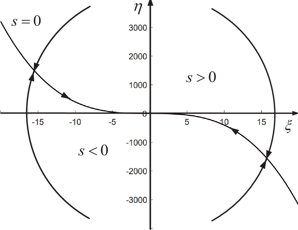
Refer to caption — Figure 1: The phase plot of the system.

In this subsection, the predefined-time stabilization problem for the uncertain second-order system is first analyzed. Consider the uncertain second-order system described as

\left\{\begin{array}[]{l}\dot{\xi}(t)=\eta(t),\\ \dot{\eta}=\tau(t)+f(t,\xi(t),\eta(t)),\end{array}\right.

(3.13)

where $\xi,\eta\in\mathbb{R}^{n}$ are the state vectors, $\tau(t)$ is the control input, and $f(t,\xi(t),\eta(t))$ denotes the uncertain term including the parametric uncertainties and external disturbances. A reasonable assumption on $f(t,\xi(t),\eta(t))$ is presented as follows.

Assumption 1.

The uncertain term $f(t,\xi(t),\eta(t))$ are bounded, i.e., there exists a positive scalar $\overline{\sigma}_{f}$ such that $\|f(t,\xi(t),\eta(t))\|\leq\overline{\sigma}_{f}$ .

Definition 1.

The main problem considered here is to design proper control input $\tau(t)$ such that system (3.13) is predefined-time stable, namely, there exists an predefined-time parameter $\mathcal{T}_{f}$ in the control design such that

\left\{\begin{array}[]{l}\mathop{\lim}\limits_{t\to{{\mathcal{T}}_{f}}}\xi(t)=0,\\ \mathop{\lim}\limits_{t\to{{\mathcal{T}}_{f}}}\eta(t)=0,\end{array}\right.

(3.14)

and $\xi(t)=0$ , $\eta(t)=0$ when $t\geq\mathcal{T}_{f}$ .

Firstly, the PTSM surface is designed as

s=\eta+\!\frac{{{{\left[\kern-3.00003pt\left[{{\textbf{1}_{n}}\!+\!{{\left[\kern-1.49994pt\left[\xi\right]\kern-1.49994pt\right]}^{2}}}\right]\kern-3.00003pt\right]}^{\frac{3}{2}}}}}{{{{\mathcal{T}}_{s}}(1-\gamma)}}\!\circ{\rm sig}{\left({\xi\circ\!{{\left[\kern-3.00003pt\left[{{\textbf{1}_{n}}\!+\!{{\left[\kern-1.49994pt\left[\xi\right]\kern-1.49994pt\right]}^{2}}}\right]\kern-3.00003pt\right]}^{-\frac{1}{2}}}}\right)^{\gamma}},

(3.15)

where $\mathcal{T}_{s}>0$ and $0<\gamma<1$ . The control input for (3.13) is designed as $\tau=\tau_{eq}+\tau_{s}$ , where $\tau_{eq}$ , $\tau_{s}$ respectively represent the equivalent control law and the nonlinear hitting control law, and are concretely presented as follows:

		$\displaystyle{\tau_{eq}}=-\frac{{3\xi\!\circ\!{{\left[\kern-3.00003pt\left[{{\textbf{1}_{n}}\!+\!{{\left[\kern-1.49994pt\left[\xi\right]\kern-1.49994pt\right]}^{2}}}\right]\kern-3.00003pt\right]}^{\frac{1}{2}}}\!\!\circ\eta}}{{{{\mathcal{T}}_{s}}(1-\gamma)}}\circ{\rm sig}{\left({\xi\!\circ\!{{\left[\kern-3.00003pt\left[{{\textbf{1}_{n}}\!+\!{{\left[\kern-1.49994pt\left[\xi\right]\kern-1.49994pt\right]}^{2}}}\right]\kern-3.00003pt\right]}^{-\frac{1}{2}}}}\right)^{\gamma}}$
		$\displaystyle\;\hskip 20.00003pt-\frac{{\gamma\eta}}{{{{\mathcal{T}}_{s}}(1-\gamma)}}\circ{\left[\kern-3.50006pt\left[{\left\|\xi\right\|\circ\!{{\left[\kern-3.00003pt\left[{{\textbf{1}_{n}}\!+\!{{\left[\kern-1.49994pt\left[\xi\right]\kern-1.49994pt\right]}^{2}}}\right]\kern-3.00003pt\right]}^{-\frac{1}{2}}}}\right]\kern-3.50006pt\right]^{\gamma-1}},$		(3.16)
		$\displaystyle{\tau_{s}}=-\frac{\pi}{{\rho{{\mathcal{T}}_{c}}}}\left({1+{{\left\\|s\right\\|}^{2\rho}}}\right)\frac{s}{{{\left\\|s\right\\|}^{\rho}}}-{\rm K}_{f}{\rm sgn}(s),$		(3.17)

where $\mathcal{T}_{c}>0$ , $0<\rho<1$ and ${\rm K}_{f}$ is a diagonal positive-definite gain matrix.

Substituting the designed control input $\tau$ into (3.13) and differentiating $s$ along (3.13) yield the following closed-loop system,

\dot{s}=-\frac{\pi}{{\rho{{\mathcal{T}}_{c}}}}\left({1+{{\left\|s\right\|}^{2\rho}}}\right)\frac{s}{{{\left\|s\right\|}^{\rho}}}-{\rm K}_{f}{\rm sgn}(s)+f(t,\xi(t),\eta(t)).

(3.18)

Further, we focus on the stability analysis of (3.18), and the corresponding theorem is presented as follows.

Theorem 2.

Utilizing the designed control input (3.16) and (3.17) for the considered uncertain system (3.13), if

		$\displaystyle\mathcal{T}_{c}>0,\hskip 10.00002pt\mathcal{T}_{s}>0,$		(3.19)
		$\displaystyle\lambda_{\min}({\rm K}_{f})\geq\overline{\sigma}_{f},$		(3.20)

then (3.13) is predefined-time stable with the predefined-time parameter being $\mathcal{T}_{f}=\mathcal{T}_{c}+\mathcal{T}_{s}$ , namely $\xi$ , $\eta$ converge to the origin within $t\leq\mathcal{T}_{f}$ .

Proof.

Construct the Lyapunov function candidate for (3.18) as $V(s)=\frac{1}{2}s^{T}s$ . It then follows that

$\displaystyle V(s)=$	$\displaystyle-\!\frac{\pi}{{\rho{{\mathcal{T}}_{c}}}}\!\!\left(\!{{{\left\\|s\right\\|}^{2\!-\!\rho}}\!\!+\!{{\left\\|s\right\\|}^{2\!+\!\rho}}}\!\right)\!-\!{s^{T}}{{\rm K}_{f}}{\rm{sgn}}(s)\!+\!{s^{T}}f$
$\displaystyle\leq$	$\displaystyle-\!\frac{\pi}{{\rho{{\mathcal{T}}_{c}}}}\!\!\left(\!{{{\left\\|s\right\\|}^{2\!-\!\rho}}\!\!+\!{{\left\\|s\right\\|}^{2\!+\!\rho}}}\!\right)\!\!-\!\left({{\lambda_{\min}}({\rm K}_{f})\!-\!\left\\|{f}\right\\|}\right)\!\left\\|s\right\\|$
$\displaystyle\leq$	$\displaystyle-\frac{\pi}{{\rho{{\mathcal{T}}_{c}}}}\!\!\left({{V^{1-\frac{\rho}{2}}}(s)+{V^{1+\frac{\rho}{2}}}(s)}\right),$	(3.21)

where $\rho\in(0,1)$ is predefined right after (3.17), (3.20) has been utilized to derive the above inequality. It thus follows from Lemma 1 that $s$ converge to the origin within predefined time $\mathcal{T}_{c}$ . Then, based on the the employment of the PTSM surface and the results in Theorem 1, one can eventually obtain that $\xi$ and $\eta$ converge to zero within $t\leq\mathcal{T}_{f}=\mathcal{T}_{c}+\mathcal{T}_{s}$ . This completes the proof

Remark 3.

The phase plot of system (3.13) using the designed algorithm is shown in Fig.1. For any chosen initial values, the trajectory $\xi(t)$ will touch the PTSM surface $s=0$ , and then converge to the origin along the PTSM surface monotonically within a predefined time.

4 Predefined-time tracking control for robot manipulators

In this section, based on the aforementioned predefined-time stability of the uncertain second-order system, we will further study the predefined-time stabilization problem of robot manipulators. To be specific, the main objective is to design proper PTSM control schemes to actuate the robot manipulator to track the desired trajectory.

4.1 System and problem formulation

The dynamics of the robot manipulator with $n$ degrees of freedoms (DOFs) can be described by the following Euler-Lagrange system,

M(q){\ddot{q}}+C(q,\dot{q}){\dot{q}}+g(q)=\tau(t)+d(t),

(4.22)

where $q$ , $\dot{q}\in\mathbb{R}^{n}$ stands for the generalized-joint coordinates and velocities, $M(q)=M_{0}(q)+\Delta M(q)\in\mathbb{R}^{n\times n}$ denotes the inertia matrix, $C(q,\dot{q})=C_{0}(q,\dot{q})+\Delta C(q,\dot{q})\in\mathbb{R}^{n\times n}$ represents the Coriolis-centrifugal matrix, $g(q)=g_{0}(q)+\Delta g(q)\in\mathbb{R}^{n}$ symbolizes the gravitational torque, $d(t)$ denotes the external disturbance, $\tau(t)$ is the torque input to be designed. Besides, $M_{0}(q)$ , $C_{0}(q,\dot{q})$ and $g_{0}(q)$ are the nominal terms with respect to $M(q)$ , $C(q,\dot{q})$ and $g(q)$ which can be used in the control design. $\Delta M(q)$ , $\Delta C(q,\dot{q})$ and $\Delta g(q)$ denote the dynamical uncertainties. Then (4.22) can be rewritten as the following form:

M_{0}(q){\ddot{q}}+C_{0}(q,\dot{q}){\dot{q}}+g_{0}(q)=\tau(t)+d(t)+h(t),

(4.23)

where $h(t)=-\Delta M(q){\ddot{q}}-\Delta C(q,\dot{q}){\dot{q}}-\Delta g(q)$ denotes the uncertain term aroused by the dynamical uncertainties. Besides, a reasonable assumption is given as follows.

Assumption 2.

The external disturbance $d(t)$ imposed on system (4.22) is upper-bounded, namely, there exists positive $\overline{\sigma}_{d}$ such that $\|d(t)\|\leq\overline{\sigma}_{d}$ .

Some properties of (4.22) are presented as follows.

Property 1.

$M(q)$ and $M_{0}(q)$ are symmetric and positive definite. Besides, $\dot{M}(q)-2C(q,\dot{q})$ and $\dot{M}_{0}(q)-2C_{0}(q,\dot{q})$ are skew symmetric, namely, for any given $\delta\in\mathbb{R}^{n}$ , it can be derived that $\delta^{T}[\dot{M}(q)-2C(q,\dot{q})]\delta=0$ and $\delta^{T}[\dot{M}_{0}(q)-2C_{0}(q,\dot{q})]\delta=0$ .

Property 2.

$M(q)$ , $C(q,\dot{q})$ , and $g(q)$ are bounded for all possible $q$ , i.e., $\|M(q)\|\leq\overline{\sigma}_{m}$ , $\|C(q,\dot{q})\|\leq\overline{\sigma}_{c}\|\dot{q}\|$ , and $\|g(q)\|\leq\overline{\sigma}_{g1}+\overline{\sigma}_{g2}\|q\|$ , where $\overline{\sigma}_{m}$ , $\overline{\sigma}_{c}$ , $\overline{\sigma}_{g1}$ , and $\overline{\sigma}_{g2}$ are positive constants.

On the other hand, the desired trajectory is denoted by ${\rm col}(q_{r},\omega_{r},\alpha_{r})$ , where $q_{r}$ , $\omega_{r}$ , and $\alpha_{r}\in\mathbb{R}^{n}$ denote the desired generalized-joint coordinate, velocity, and acceleration of the referenced trajectory, i.e., ${{\dot{q}}_{r}}={\omega_{r}}$ , ${{\dot{\omega}}_{r}}={\alpha_{r}}$ . A mild assumption on the acceleration of the referenced trajectory is presented as follows.

Assumption 3.

The acceleration of the referenced trajectory is bounded, namely $\|\alpha_{r}\|\leq\overline{\sigma}_{\alpha}$ , where $\overline{\sigma}_{\alpha}$ is a positive constant.

Definition 2.

The zero-error predefined-time stabilization problem for robot manipulators is solved if there exists an predefined-time parameter $\mathcal{T}_{f}$ in the control design such that

\left\{\begin{array}[]{l}\mathop{\lim}\limits_{t\to{{\mathcal{T}}_{f}}}\|e\|=0,\\ \mathop{\lim}\limits_{t\to{{\mathcal{T}}_{f}}}\|\dot{e}\|=0,\end{array}\right.

(4.24)

and $\|e\|=0$ , $\|\dot{e}\|=0$ for $t\geq\mathcal{T}_{f}$ , where $e=q-q_{d}$ and $\dot{e}=\dot{q}-\omega_{d}$ denote the errors states. Especially, the practical predefined-time stabilization problem is solved if

\left\{\begin{array}[]{l}\mathop{\lim}\limits_{t\to{{\mathcal{T}}_{f}}}\|e\|\leq\delta_{1},\\ \mathop{\lim}\limits_{t\to{{\mathcal{T}}_{f}}}\|\dot{e}\|\leq\delta_{2},\end{array}\right.

(4.25)

and $\|e\|\leq\delta_{1}$ , $\|\dot{e}\|\leq\delta_{2}$ for $t\geq\mathcal{T}_{f}$ , where $\delta_{1}$ , $\delta_{2}>0$ can be adjusted by appropriate control parameters.

4.2 Control design and stability analysis

Based on Property 2 and Assumption 2, it can be derived that $\|M_{0}(q)\|\leq\overline{\sigma}_{m0}$ , and $\|h(t)\|\leq\overline{\sigma}_{1}+\overline{\sigma}_{2}\|q\|+\overline{\sigma}_{3}\|\dot{q}\|^{2}$ , where $\overline{\sigma}_{m0}$ , $\overline{\sigma}_{1}$ , $\overline{\sigma}_{2}$ , and $\overline{\sigma}_{3}$ are positive constants. Design the PTSM vector as

s=\dot{e}+\frac{{{{\left[\kern-3.00003pt\left[{{\textbf{1}_{n}}\!+\!{{\left[\kern-1.49994pt\left[e\right]\kern-1.49994pt\right]}^{2}}}\right]\kern-3.00003pt\right]}^{\frac{3}{2}}}}}{{{{\mathcal{T}}_{s}}(1-\gamma)}}\!\circ{\rm sig}{\left({e\circ\!{{\left[\kern-3.00003pt\left[{{\textbf{1}_{n}}\!+\!{{\left[\kern-1.49994pt\left[e\right]\kern-1.49994pt\right]}^{2}}}\right]\kern-3.00003pt\right]}^{-\frac{1}{2}}}}\right)^{\gamma}},

(4.26)

where $\mathcal{T}_{s}>0$ , and $0<\gamma<1$ . For simplification, $M_{0}$ , $C_{0}$ , and $g_{0}$ are applied to respectively denote $M_{0}(q)$ , $C_{0}(q,\dot{q})$ , and $g_{0}(q)$ in the following presentation. Then the PTSM controller $\tau(t)=\tau_{eq}+\tau_{s}$ is presented as follows:

		$\displaystyle{\tau_{eq}}=-{M_{0}}\!\!\left[\!\frac{{3e\!\circ\!{{\left[\kern-3.00003pt\left[\!{{\textbf{1}_{n}}\!+\!{{\left[\kern-1.49994pt\left[e\right]\kern-1.49994pt\right]}^{2}}}\!\right]\kern-3.00003pt\right]}^{\frac{1}{2}}}\!\!\circ\!\dot{e}}}{{{{\mathcal{T}}_{s}}(1-\gamma)}}\!\circ\!{\rm sig}{{\left(\!\!{x\!\circ\!{{\left[\kern-3.00003pt\left[\!{{\textbf{1}_{n}}\!+\!{{\left[\kern-1.49994pt\left[e\right]\kern-1.49994pt\right]}^{2}}}\!\right]\kern-3.00003pt\right]}^{-\frac{1}{2}}}}\!\right)}^{\gamma}}\right.$
		$\displaystyle\hskip 20.00003pt\;\left.+\frac{{\gamma\dot{e}}}{{{{\mathcal{T}}_{s}}(1\!-\!\gamma)}}\!\circ\!{{\left[\kern-3.50006pt\left[\!{\left\|e\right\|\!\circ\!{{\left[\kern-3.00003pt\left[{{\textbf{1}_{n}}\!+\!{{\left[\kern-1.49994pt\left[e\right]\kern-1.49994pt\right]}^{2}}}\right]\kern-3.00003pt\right]}^{-\frac{1}{2}}}}\!\right]\kern-3.50006pt\right]}^{\gamma\!-\!1}}\right]\!+\!{C_{0}}\dot{q}\!+\!{g_{0}},$		(4.27)
		$\displaystyle{\tau_{s}}=-\frac{\pi}{{\rho{{\mathcal{T}}_{c}}}}\left({\hat{\sigma}_{m0}^{1-\frac{\rho}{2}}+\hat{\sigma}_{m0}^{1+\frac{\rho}{2}}{{\left\\|s\right\\|}^{2\rho}}}\right)\frac{s}{{{\left\\|s\right\\|}^{\rho}}}-C_{0}s$
		$\displaystyle\hskip 20.00003pt-\left[{\left({{{\overline{\sigma}}_{1}}\!+\!{{\overline{\sigma}}_{2}}\left\\|q\right\\|\!+\!{{\overline{\sigma}}_{3}}{{\left\\|{\dot{q}}\right\\|}^{2}}}\right){I_{\rm{n}}}\!+\!{{\rm K}_{d}}}\right]{\mathop{\rm sgn}}(s),$		(4.28)

where $\hat{\sigma}_{m0}=\frac{1}{2}\overline{\sigma}_{m0}$ , $\mathcal{T}_{c}>0$ , $0<\rho<1$ , and ${\rm K}_{d}$ is a diagonal positive-definite gain matrix. Then, substituting (4.27) and (4.28) into (4.23) yields the following closed-loop system,

	$\displaystyle\dot{s}=$	$\displaystyle\!-M_{0}^{-1}\!\left\{\frac{\pi}{{\rho{{\mathcal{T}}_{c}}}}\left(\!{\hat{\sigma}_{m0}^{1-\frac{\rho}{2}}\!\!+\!\hat{\sigma}_{m0}^{1+\frac{\rho}{2}}{{\left\\|s\right\\|}^{2\rho}}}\!\right)\!\frac{s}{{{\left\\|s\right\\|}^{\rho}}}\!-\!d(t)\!-\!h(t)\right.$
		$\displaystyle\!+\!C_{0}s\!+\!\!\left.\left[{\left({{{\overline{\sigma}}_{1}}\!+\!{{\overline{\sigma}}_{2}}\!\left\\|q\right\\|\!+\!{{\overline{\sigma}}_{3}}\!{{\left\\|{\dot{q}}\right\\|}^{2}}}\right)\!{I_{n}}\!+\!{{\rm K}_{d}}}\right]{\mathop{\rm sgn}}(s)\!\right\}\!-\!\alpha_{r}$		(4.29)

Theorem 3.

Suppose that Assumptions 2 and 3 hold. Utilizing the PTSM controller (4.27) and (4.28) for (4.22), if

		$\displaystyle\mathcal{T}_{c}>0,\hskip 10.00002pt\mathcal{T}_{s}>0,$		(4.30)
		$\displaystyle\lambda_{\min}({{\rm K}_{d}})\geq\overline{\sigma}_{d}+\overline{\sigma}_{m0}\overline{\sigma}_{\alpha},$		(4.31)

then the zero-error predefined-time stabilization problem for the robot manipulator can be addressed within $t\leq\mathcal{T}_{c}+\mathcal{T}_{s}$ .

Proof.

Construct $V(s)=\frac{1}{2}s^{T}M_{0}s$ as the Lyapunov function for (4.29). According to Property 1, $V(s)$ is positive-definite. Then, differentiating $V(s)$ along (4.29) yields that

$\displaystyle\dot{V}(s)$	$\displaystyle=s^{T}M_{0}\dot{s}+\frac{1}{2}s^{T}\dot{M}_{0}s$
	$\displaystyle\leq\!\!-\frac{\pi}{{\rho{{\mathcal{T}}_{c}}}}\!\!\left(\!{\hat{\sigma}_{m0}^{1-\frac{\rho}{2}}{{\left\\|s\right\\|}^{2-\rho}}\!\!+\!\hat{\sigma}_{m0}^{1+\frac{\rho}{2}}{{\left\\|s\right\\|}^{2+\rho}}}\!\right)\!\!+\!\frac{1}{2}s^{T}(\dot{M}_{0}\!-\!2C_{0})s$
	$\displaystyle\!\hskip 10.00002pt-\left({{{\overline{\sigma}}_{1}}+{{\overline{\sigma}}_{2}}\left\\|q\right\\|+{{\overline{\sigma}}_{3}}{{\left\\|{\dot{q}}\right\\|}^{2}}+{\lambda_{\min}}({{\rm{K}}_{d}})}\right)\left\\|s\right\\|$
	$\displaystyle\!\hskip 10.00002pt+\left({\left\\|{h(t)}\right\\|+\left\\|{d(t)}\right\\|+\left\\|M_{0}\right\\|\left\\|{{\alpha_{d}}}\right\\|}\right)\left\\|s\right\\|$
	$\displaystyle\!\leq-\frac{\pi}{{\rho{{\mathcal{T}}_{c}}}}\left({\hat{\sigma}_{m0}^{1-\frac{\rho}{2}}{{\left\\|s\right\\|}^{2-\rho}}+\hat{\sigma}_{m0}^{1+\frac{\rho}{2}}{{\left\\|s\right\\|}^{2+\rho}}}\right)$
	$\displaystyle\!\hskip 10.00002pt-\left({{\lambda_{\min}}({{\rm{K}}_{d}})-\overline{\sigma}_{d}-\overline{\sigma}_{m0}\overline{\sigma}_{\alpha}}\right)\left\\|s\right\\|$
	$\displaystyle\!\leq-\frac{\pi}{{\rho{{\mathcal{T}}_{c}}}}\left({\hat{\sigma}_{m0}^{1-\frac{\rho}{2}}{{\left\\|s\right\\|}^{2-\rho}}+\hat{\sigma}_{m0}^{1+\frac{\rho}{2}}{{\left\\|s\right\\|}^{2+\rho}}}\right),$	(4.32)

where $\rho\in(0,1)$ is predefined right after (4.28), Properties 1-2 and (4.31) has been applied to obtain the above inequality. Note that $V(s)\leq\hat{\sigma}_{m0}\|s\|^{2}$ due to that $\|M_{0}(q)\|\leq 2\hat{\sigma}_{m0}$ . It then follows that

\dot{V}(s)\leq-\frac{\pi}{{\rho{{\mathcal{T}}_{c}}}}\left({{V^{1-\frac{\rho}{2}}}(s)+{V^{1+\frac{\rho}{2}}}(s)}\right).

(4.33)

Thus, based on Lemma 1 and the analysis in Theorem 1, it can be derived that the tracking errors $e$ and $\dot{e}$ converge to the origin within the predefined time $t\leq\mathcal{T}_{f}=\mathcal{T}_{s}+\mathcal{T}_{c}$ . This completes the proof.

Remark 4.

Note that the tracking errors in [17] finally converge to a bounded set within the setting time, due to the adoption of the linear sliding surface. Thus, it is of great significance to design the PTSM surface (3.9), based on which the PTSM controller is proposed to successfully solve the zero-error predefined-time tracking problem for robot manipulators.

Remark 5.

Inspired by [23], we further give the following TBG-based controller to address the practical predefined-time tracking problem for robot manipulators: $\tau=\tau_{eq}+\tau_{s}$ , where $\tau_{eq}$ is designed as same as (4.27) and $\tau_{s}$ is designed as

	$\displaystyle{\tau_{s}}=$	$\displaystyle-\left[{\left({{{\overline{\sigma}}_{1}}+{{\overline{\sigma}}_{2}}\left\\|q\right\\|+{{\overline{\sigma}}_{3}}{{\left\\|{\dot{q}}\right\\|}^{2}}}\right){I_{\rm{n}}}+{{\rm{K}}_{d}}}\right]{\mathop{\rm sgn}}(s)-{C_{0}}s$
		$\displaystyle-\frac{{{\hat{\sigma}}_{m0}}{\dot{\varepsilon}(t)}}{{1-\varepsilon(t)+\epsilon}}s,$		(4.34)

where $\varepsilon(t)$ is the TBG, $\hat{\sigma}_{m0}$ is the same as that in (4.28), $0<\epsilon\ll 1$ , and ${\rm K}_{d}$ is a diagonal positive-definite gain matrix.

Corollary 1.

Suppose that Assumptions 2 and 3 hold. Utilizing the TBG-based controller (4.27) and (4.34) for (4.22), if $\varepsilon(t)$ is give as in Lemma 2, and

		$\displaystyle\mathcal{T}_{c}>0,\hskip 10.00002pt\mathcal{T}_{s}>0,$
		$\displaystyle\lambda_{\min}({\rm K}_{d})\geq\overline{\sigma}_{d}+\overline{\sigma}_{m0}\overline{\sigma}_{\alpha},$		(4.35)

where $\mathcal{T}_{c}$ is the control parameter in $\varepsilon(t)$ , then the practical predefined-time stabilization problem of the robot manipulator can be addressed within $t\leq\mathcal{T}_{c}+\mathcal{T}_{s}$ .

Proof.

Substituting (4.27) and (4.34) into (4.22), and differentiating $s$ along (4.22) yield below closed-loop system:

	$\displaystyle\dot{s}=$	$\displaystyle-M_{0}^{-1}\left\{\frac{{{\hat{\sigma}}_{m0}}{\dot{\varepsilon}(t)}}{{1-\varepsilon(t)+\epsilon}}s-d(t)-h(t)+{C_{0}}s\right.$
		$\displaystyle\left.+\left[{\left({{{\overline{\sigma}}_{1}}+{{\overline{\sigma}}_{2}}\left\\|q\right\\|+{{\overline{\sigma}}_{3}}{{\left\\|{\dot{q}}\right\\|}^{2}}}\right){I_{\rm{n}}}+{{\rm{K}}_{d}}}\right]{\rm{sgn}}(s)\right\}-{\alpha_{r}}.$		(4.36)

Select $V(s)=\frac{1}{2}s^{T}M_{0}s$ . It then follows that

$\displaystyle\dot{V}(s)$	$\displaystyle={s^{T}}{M_{0}}\dot{s}+\frac{1}{2}{s^{T}}{{\dot{M}}_{0}}s$
	$\displaystyle\leq-\frac{{{{\hat{\sigma}}_{m0}}\dot{\varepsilon}(t)}}{{1\!-\!\varepsilon(t)\!+\!\epsilon}}{\left\\|s\right\\|^{2}}\!-\!\left({{\lambda_{\min}}({{\rm{K}}_{d}})\!-\!{{\overline{\sigma}}_{d}}\!-\!{{\overline{\sigma}}_{m0}}{{\overline{\sigma}}_{\alpha}}}\right)\left\\|s\right\\|$
	$\displaystyle\leq-\frac{{\dot{\varepsilon}(t)}}{{1-\varepsilon(t)+\epsilon}}V(s).$	(4.37)

Based on Lemma 2, it can be derived that $V(s)$ converges to a bounded set $\Omega=\{V(s)|V(s)\leq\frac{\epsilon}{1+\epsilon}V(s(0))\}$ at $\mathcal{T}_{c}$ . It then follows from $V(s)\geq\frac{\lambda_{\min}(M_{0})}{2}\|s\|^{2}$ that ${\lim_{t\to{{\mathcal{T}}_{c}}}}\left\|s\right\|\leq\delta$ , where $\delta=\sqrt{\frac{2\epsilon}{{{\lambda_{\min}}({M_{0}})(1+\epsilon)}}V(s(0))}$ . As is shown in Fig.2, the error vectors will converge to a bounded neighborhood of the origin, which is related with $\delta$ , in a predefined time $\mathcal{T}_{s}$ . To be specific, the less $\delta$ , the higher tracking performance we derive. Besides, it is noteworthy that $\delta$ can be adjusted by selecting proper $\epsilon$ . Then, we can choose a small enough parameter $\epsilon$ to derive satisfactory tracking performance. Thus, it can be concluded that the practical predefined-time stabilization problem of robot manipulators is addressed with the predefined time being $\mathcal{T}_{c}+\mathcal{T}_{s}$ . This completes the proof.

Remark 6.

Redesign the nonlinear hitting control law $\tau_{s}$ as

	$\displaystyle\tau_{s}=$	$\displaystyle-{C_{0}}s-\left[{\left({{{\overline{\sigma}}_{1}}+{{\overline{\sigma}}_{2}}\left\\|q\right\\|+{{\overline{\sigma}}_{3}}{{\left\\|{\dot{q}}\right\\|}^{2}}}\right){I_{\rm{n}}}+{{\rm K}_{d}}}\right]{\mathop{\rm sgn}}(s)$
		$\displaystyle-\alpha{\hat{\sigma}_{m0}^{\frac{m_{1}+n_{1}}{2n_{1}}}}{s^{\frac{{{m_{1}}}}{{{n_{1}}}}}}-\beta{\hat{\sigma}_{m0}^{\frac{m_{2}+n_{2}}{2n_{2}}}}{s^{\frac{{{m_{2}}}}{{{n_{2}}}}}},$		(4.38)

where $\hat{\sigma}_{m0}$ is the same as that in (4.28), $\alpha,\beta>0$ , $m_{1},n_{1},m_{2}$ and $n_{2}$ are positive integers with $m_{1}>n_{1}$ and $m_{2}<n_{2}$ . The main results thus can degrade into fixed-time convergence, and the corresponding corollary is given as follows.

Corollary 2.

Suppose that Assumptions 2 and 3 hold. Utilizing the TSM controller (4.27) and (4.38) for (4.22), if (4.31) hold and $\mathcal{T}_{s}>0$ , then $e_{i}$ and $\dot{e}_{i}$ converge to zero in fixed-time, and the settling time function is given as

\displaystyle\mathcal{T}\leq\mathcal{T}_{s}+\frac{2n_{1}}{{\alpha\left({{m_{1}}-{n_{1}}}\right)}}+\frac{{{n_{2}}+{m_{2}}}}{{\beta\left({{n_{2}}-{m_{2}}}\right)}}.

(4.39)

Proof.

Substituting (4.27) and (4.38) into (4.22) yields the following closed-loop system,

	$\displaystyle\dot{s}=$	$\displaystyle-\!M_{0}^{-1}\!\left\{\!\alpha{\hat{\sigma}_{m0}^{\frac{m_{1}+n_{1}}{2n_{1}}}}\!\!{s^{\frac{{{m_{1}}}}{{{n_{1}}}}}}\!\!+\!\beta{\hat{\sigma}_{m0}^{\frac{m_{2}+n_{2}}{2n_{2}}}}\!\!{s^{\frac{{{m_{2}}}}{{{n_{2}}}}}}\!\!-\!d(t)\!-\!h(t)\!+\!{C_{0}}s\right.$
		$\displaystyle\left.+\!\left[{\left({{{\overline{\sigma}}_{1}}+{{\overline{\sigma}}_{2}}\left\\|q\right\\|+{{\overline{\sigma}}_{3}}{{\left\\|{\dot{q}}\right\\|}^{2}}}\right){I_{\rm{n}}}+{{\rm{K}}_{d}}}\right]{\rm{sgn}}(s)\right\}-{\alpha_{r}}.$		(4.40)

Construct the Lyapunov function as $V(s)=\frac{1}{2}s^{T}M_{0}s$ . Then, differentiating $V(s)$ along (4.40) yields that

$\displaystyle\dot{V}(s)\leq$	$\displaystyle-\alpha\hat{\sigma}_{m0}^{\frac{{{m_{1}}+{n_{1}}}}{{2{n_{1}}}}}{\left\\|s\right\\|^{\frac{{{m_{1}}+{n_{1}}}}{{{n_{1}}}}}}-\beta\hat{\sigma}_{m0}^{\frac{{{m_{2}}+{n_{2}}}}{{2{n_{2}}}}}{\left\\|s\right\\|^{\frac{{{m_{2}}+{n_{2}}}}{{{n_{2}}}}}}$
	$\displaystyle-\left({{\lambda_{\min}}({{\rm{K}}_{d}})-{{\overline{\sigma}}_{d}}-{{\overline{\sigma}}_{m0}}{{\overline{\sigma}}_{\alpha}}}\right)\left\\|s\right\\|$
$\displaystyle\leq$	$\displaystyle-\alpha{V^{\frac{{{m_{1}}+{n_{1}}}}{{2{n_{1}}}}}}(s)-\beta{V^{\frac{{{m_{2}}+{n_{2}}}}{{2{n_{2}}}}}}(s).$	(4.41)

Thus, it can be concluded that $s$ converges to the origin within $t\leq\frac{2n_{1}}{{\alpha\left({{m_{1}}-{n_{1}}}\right)}}+\frac{{{n_{2}}+{m_{2}}}}{{\beta\left({{n_{2}}-{m_{2}}}\right)}}$ . It follows that $e$ and $\dot{e}$ converge to zero within $t\leq\mathcal{T}_{s}+\frac{2n_{1}}{{\alpha\left({{m_{1}}-{n_{1}}}\right)}}+\frac{{{n_{2}}+{m_{2}}}}{{\beta\left({{n_{2}}-{m_{2}}}\right)}}$ . This completes the proof.

5 Simulation Examples

In this section, several simulation experiments are conducted to verify the effectiveness of the main results.

5.1 Simulation for the uncertain second-order system

We first conduct simulation experiment on uncertain second-order system to verify the predefined-time stability presented in Theorem 2.

Example 1.

The designed PTSM controller (3.16) and (3.17) is used to stabilize the uncertain second-order system (3.13). Choose the state vectors $\xi,\eta\in\mathbb{R}^{2}$ , and the control parameters as $\gamma=0.5$ , $\rho=0.4$ , $\mathcal{T}_{s}=4$ , $\mathcal{T}_{c}=6$ , and ${\rm K}_{f}=10$ . Besides, the uncertain term $f(t,\xi(t),\eta(t))$ is selected as a random function bounded by $5$ . Ten groups of initial value $\xi(0)$ and $\eta(0)$ are randomly chosen in $[-15,15]$ .

Simulation Results: The simulation results are shown in Figs.3 and 4. It can be observed in Fig 3 that the states $\xi$ and $\eta$ converge to the origin within the predefined time $\mathcal{T}_{f}=\mathcal{T}_{s}+\mathcal{T}_{c}=10s$ for any given initial values. Similarly, Fig. 4 shows the predefined-time convergence of the PTSM vector $s$ .

5.2 Simulations for the robot manipulators

In this subsection, we select the 2-DOF robot manipulator to verify the effectiveness of the main results in Theorem 3 and Corollary 1. The specific dynamics is presented as follows:

\displaystyle\left[\!\!{\begin{array}[]{*{20}{c}}{M_{11}}&{M_{12}}\\ {M_{21}}&{M_{22}}\end{array}}\!\!\right]\!\left[\!\!\begin{array}[]{l}{{\ddot{q}}_{1}}\\ {{\ddot{q}}_{2}}\end{array}\!\!\right]\!+\!\left[\!\!{\begin{array}[]{*{20}{c}}{C_{11}}&{C_{12}}\\ {C_{21}}&{C_{22}}\end{array}}\!\!\right]\!\left[\!\!\begin{array}[]{l}{{\dot{q}}_{1}}\\ {{\dot{q}}_{2}}\end{array}\!\!\right]\!+\!\left[\!\!\begin{array}[]{l}{g_{1}}\\ {g_{2}}\end{array}\!\!\right]\!=\!\left[\!\!\!\begin{array}[]{l}{\tau_{1}}\\ {\tau_{2}}\end{array}\!\!\right]\!+\!\left[\!\!\begin{array}[]{l}{d_{1}}(t)\\ {d_{2}}(t)\end{array}\!\!\right],

where $M_{11}=p_{i1}+2{p_{2}}\cos(q_{2})$ , $M_{12}=M_{21}=p_{3}+p_{2}\cos(q_{2})$ , $M_{22}=p_{3}$ , $C_{11}=-{p_{2}}\sin({q_{2}}){\dot{q}_{2}}$ , $C_{12}=-{p_{2}}\sin(q_{2})(\dot{q}_{1}+\dot{q}_{2})$ , $C_{21}={p_{2}}\sin(q_{2}){\dot{q}_{1}}$ , $C_{22}=0$ , $g_{1}=g{p_{4}}{\cos(q_{1})}+g{p_{5}}{\cos(q_{1}+q_{2})}$ , $g_{2}=g{p_{5}}{\cos(q_{1}+q_{2})}$ , $p_{1}=m_{1}{r_{1}^{2}}+m_{2}(l_{1}^{2}+r_{2}^{2})+I_{1}+I_{2}$ , $p_{2}=m_{2}{l_{1}}{r_{2}}$ , $p_{3}=m_{2}{r_{2}^{2}}+I_{2}$ , $p_{4}=m_{1}r_{1}+m_{2}l_{1}$ , $p_{5}=m_{2}r_{2}$ , $I_{1}=\frac{1}{3}{m_{1}}l_{1}^{2}$ , $I_{2}=\frac{1}{3}{m_{2}}l_{2}^{2}$ , $g=9.8m/s^{2}$ is the gravitational constant, $m,l,r$ are the physical parameters, which are selected as $m=[2.8,1.8]^{T}{\rm kg}$ , $l=[3.8,2.8]^{T}{\rm m}$ , and $r=\frac{1}{2}l$ . Besides the estimated value of the corresponding physical parameters are given as $\hat{m}=[2.75,1.85]^{T}{\rm kg}$ , $\hat{l}=[3.86,2.74]^{T}{\rm m}$ , and $\hat{r}=\frac{1}{2}\hat{l}$ . On the other hand, the trajectory of the referenced trajectory is chosen as

\left\{\begin{array}[]{l}{q_{r}}={[7+5\sin(t),-7-5\cos(t)]^{T}},\\ {{\dot{q}}_{r}}={[5\cos(t),5\sin(t)]^{T}}.\end{array}\right.

(5.42)

Example 2.

The PTSM controller (4.27) and (4.28) is used for system (4.22) to solve the zero-error predefined-time tracking problem. The control parameters are selected as $\gamma=0.5$ , $\rho=0.5$ , $\overline{\sigma}_{1}=14$ , $\overline{\sigma}_{2}=12$ , $\overline{\sigma}_{3}=10$ , ${\rm K}_{d}=25I_{2}$ , and $\overline{\sigma}_{m0}=5$ to make the corresponding assumptions and sufficient conditions hold. Besides, the external disturbance is selected as a random function bounded by $5$ . Besides, we select $\mathcal{T}_{s}=4$ , $\mathcal{T}_{c}=6$ , and $\mathcal{T}_{s}=1$ , $\mathcal{T}_{c}=1$ to respectively carry out the simulation experiment with the initial values chosen randomly in $[-5,5]$ .

Example 3.

The TBG-based controller (4.27) and (4.34) is used for system (4.22) to solve the practical predefined-time tracking problem. The TBG $\varepsilon(t)$ is selected as follows to make the conditions in Lemma 2 hold,

\varepsilon(t)=\left\{\begin{array}[]{l}\frac{{10}}{{{6^{6}}}}{t^{6}}-\frac{{24}}{{{6^{6}}}}{t^{5}}+\frac{{15}}{{{6^{4}}}}{t^{4}},\;\;t\in\left[{0,{{\mathcal{T}}_{c}}}\right],\\ 1,\qquad\qquad\qquad\qquad t\in\left({{{\mathcal{T}}_{c}},+\infty}\right),\end{array}\right.

where $\mathcal{T}_{c}=6$ . Besides, select $\epsilon=0.1$ , $\mathcal{T}_{s}=4$ , and the remain settings are given as the same as that in Example 2.

Simulation Results: The simulation results are shown in Figs.5-9. To be specific, Figs.5-6 and Figs.7-8 respectively show that the predefined-time tracking control for the 2-DOF manipulator can be realized by employing both the PTSM controller (4.27), (4.28) and the TBG-based controller (4.27), (4.34). Besides, it can be seen from the tracking errors shown in Figs.6 and 8 that using the PTSM controller (4.27), (4.28) derives higher tracking performance than using the TBG-based controller (4.27), (4.34), which is consistent with the main results that using (4.27), (4.28) and (4.27), (4.34) respectively solve the zero-error and practical predefined-time tracking problems for the robot manipulator. Next, comparisons of the total energy consumed by using the three different control algorithms in this paper have been made based on a metric of $E=\int_{0}^{10}{\left\|{\tau(t)}\right\|}dt$ , and the results is shown in Fig.9, from which we can derive that the TBG-based controller can effectively reduce the energy consumption. In conclusion, the main results presented in Theorems 1-3 are theoretically correct.

6 Conclusion

This paper has presented a novel PTSM surface to design a new control scheme for stabilizing the tracking errors of the robot manipulator to the origin in a predefined time. The sufficient conditions on the control parameters for guaranteeing zero-error predefined-time stability of the closed-loop system have been derived by carrying out the formal systemic analysis. It is observed from the comparison studies that the PTSM control scheme provides better tracking performance while the TBG-based ones consumes less energy. Finally, the simulation results have shown the satisfactory steady-error performance. Future work will be focused on the predefined-time stabilization problem of robot manipulators in task space.

References

[1] X. Liu, X. Su, P. Shi, C. Shen, and Y. Peng, “Event-triggered sliding mode control of nonlinear dynamic systems.” Automatica, to be published, doi: 10.1016/j.automatica.2019.108738.
[2] F. Li, C. Du, C. Yang, L. Wu, and W. Gui, “Finite-time asynchronous sliding mode control for Markovian jump systems.” Automatica, to be published, doi: doi.org/10.1016/j.automatica.2019.108503.
[3] H. Li, P. Shi, and D. Yao, “Adaptive sliding-mode control of Markov jump nonlinear systems with actuator faults.” IEEE Transactions on Automatic Control, vol. 62, no. 4, pp. 1933-1939, 2016. 62(4), 1933-1939.
[4] N. Wang, H. R. Karimi, H. Li, and S. Su, “Accurate trajectory tracking of disturbed surface vehicles: a finite-time control approach.” IEEE/ASME Transactions on Mechatronics, to be published, doi: 10.1109/TMECH.2019.2906395.
[5] M. F. Ge, Z. W. Liu, G. Wen, X. Yu, and T. Huang, “Hierarchical controller-estimator for coordination of networked Euler-Lagrange systems.” IEEE Transactions on Cybernetics, to be published. doi: 10.1109/TCYB.2019.2914861.
[6] C. D. Liang, L. Wang, X. Y. Yao, Z. W. Liu, and M. F. Ge, “Multi-target tracking of networked heterogeneous collaborative robots in task space.” Nonlinear Dynamics, vol. 97, no. 2, pp. 1159-1173, 2019.
[7] Z. Wang, B. Liang, Y. Sun, and T. Zhang, “Adaptive fault-tolerant prescribed-time control for teleoperation systems with position error constraints.” IEEE Transactions on Industrial Informatics, to be published, doi: 10.1109/TII.2019.2951329.
[8] Z. Meng, D. V. Dimarogonas, and K. H. Johansson, “Leader-follower coordinated tracking of multiple heterogeneous Lagrange systems using continuous control.” IEEE Transactions on Robotics, vol. 30, no. 3, pp. 739-745, 2013.
[9] T. F. Ding, M. F. Ge, Z. W. Liu, Y. W. Wang, and H. R. Karimi, “Discrete-communication-based bipartite tracking of networked robotic systems via hierarchical hybrid control.” IEEE Transactions on Circuits and Systems I: Regular Papers, to be published, doi: 10.1109/TCSI.2019.2961804.
[10] Y. Sun, L. Chen, G. Ma, and C. Li, “Adaptive neural network tracking control for multiple uncertain Euler-Lagrange systems with communication delays.” Journal of the Franklin Institute, vol. 354, no. 7, pp. 2677-2698, 2017.
[11] W. He, Y. Chen, and Z. Yin, “Adaptive neural network control of an uncertain robot with full-state constraints.” IEEE Transactions on Cybernetics, vol. 46 no. 3, pp. 620-629, 2015.
[12] Z. Meng, W. Ren, and Z. You, “Distributed finite-time attitude containment control for multiple rigid bodies.” Automatica, vol. 46, no. 12, pp. 2092-2099, 2010.
[13] Y. Feng, X. Yu, and Z. Man, “Non-singular terminal sliding mode control of rigid manipulators.” Automatica, vol. 38, no. 12, pp. 2159-2167, 2002.
[14] S. Yu, X. Yu, B. Shirinzadeh, and Z. Man, “Continuous finite-time control for robotic manipulators with terminal sliding mode.” Automatica, vol. 41, no. 11, pp. 1957-1964, 2005.
[15] Z. Zuo, “Nonsingular fixed-time consensus tracking for second-order multi-agent networks.” Automatica, vol. 54, pp. 305-309, 2015.
[16] Z. Zuo, “Non-singular fixed-time terminal sliding mode control of non-linear systems.” IET Control Theory & Applications, vol. 9, no. 4, pp. 545-552, 2014.
[17] A. J. Munoz-Vazquez, J. D. Sanchez-Torres, E. J. Rodriguez, and A. Loukianov, “Predefined-time robust stabilization of robotic manipulators.” IEEE/ASME Transactions on Mechatronics, to be published, doi:10.1109/TMECH.2019.2906289.
[18] A. J. Munoz-Vazquez, J. D. Sanchez-Torres, S. Gutierrez-Alcala, E. Jimenez-Rodriguez, and A. G. Loukianov, “Predefined-time robust contour tracking of robotic manipulators.” Journal of the Franklin Institute, vol. 356, no. 5, pp. 2709-2722, 2019.
[19] J. D. Sanchez-Torres, M. Defoort, and A. J. Munoz-Vazquez, (2019). “Predefined-time stabilisation of a class of nonholonomic systems.” International Journal of Control, to be published, doi: 10.1080/00207179.2019.1569262.
[20] R. Aldana-Lopez, D. Gomez-Gutierrez, M. Defoort, J. D. Sanchez-Torres, and A. J. Munoz-Vazquez, “A class of robust consensus algorithms with predefined-time convergence under switching topologies.” International Journal of Robust and Nonlinear Control, vol. 29, no. 17, pp. 6179-6198, 2019.
[21] Y. Wang, Y. Song, D. J. Hill, and M. Krstic, “Prescribed-time consensus and containment control of networked multiagent systems.” IEEE Transactions on Cybernetics, vol. 49, no. 4, pp. 1138-1147, 2018.
[22] Y. Hong, J. Huang, and Y. Xu, “On an output feedback finite-time stabilization problem.” IEEE Transactions on Automatic Control, vol. 46, no. 2, pp. 305-309, 2001.
[23] B. Ning, Q. L. Han, and Z. Zuo, “Practical fixed-time consensus for integrator-type multi-agent systems: A time base generator approach.” Automatica, vol. 105, pp. 406-414, 2019.

$\displaystyle\dot{V}(s)$	$\displaystyle=s^{T}M_{0}\dot{s}+\frac{1}{2}s^{T}\dot{M}_{0}s$
	$\displaystyle\leq\!\!-\frac{\pi}{{\rho{{\mathcal{T}}_{c}}}}\!\!\left(\!{\hat{\sigma}_{m0}^{1-\frac{\rho}{2}}{{\left\\|s\right\\|}^{2-\rho}}\!\!+\!\hat{\sigma}_{m0}^{1+\frac{\rho}{2}}{{\left\\|s\right\\|}^{2+\rho}}}\!\right)\!\!+\!\frac{1}{2}s^{T}(\dot{M}_{0}\!-\!2C_{0})s$
	$\displaystyle\!\hskip 10.00002pt-\left({{{\overline{\sigma}}_{1}}+{{\overline{\sigma}}_{2}}\left\\|q\right\\|+{{\overline{\sigma}}_{3}}{{\left\\|{\dot{q}}\right\\|}^{2}}+{\lambda_{\min}}({{\rm{K}}_{d}})}\right)\left\\|s\right\\|$
	$\displaystyle\!\hskip 10.00002pt+\left({\left\\|{h(t)}\right\\|+\left\\|{d(t)}\right\\|+\left\\|M_{0}\right\\|\left\\|{{\alpha_{d}}}\right\\|}\right)\left\\|s\right\\|$
	$\displaystyle\!\leq-\frac{\pi}{{\rho{{\mathcal{T}}_{c}}}}\left({\hat{\sigma}_{m0}^{1-\frac{\rho}{2}}{{\left\\|s\right\\|}^{2-\rho}}+\hat{\sigma}_{m0}^{1+\frac{\rho}{2}}{{\left\\|s\right\\|}^{2+\rho}}}\right)$
	$\displaystyle\!\hskip 10.00002pt-\left({{\lambda_{\min}}({{\rm{K}}_{d}})-\overline{\sigma}_{d}-\overline{\sigma}_{m0}\overline{\sigma}_{\alpha}}\right)\left\\|s\right\\|$
	$\displaystyle\!\leq-\frac{\pi}{{\rho{{\mathcal{T}}_{c}}}}\left({\hat{\sigma}_{m0}^{1-\frac{\rho}{2}}{{\left\\|s\right\\|}^{2-\rho}}+\hat{\sigma}_{m0}^{1+\frac{\rho}{2}}{{\left\\|s\right\\|}^{2+\rho}}}\right),$	(4.32)

Predefined-time Terminal Sliding Mode Control of Robot Manipulatorsfootnoteinfo

Abstract

keywords

1 Introduction

2 Preliminaries

2.1 Conventional terminal sliding mode surface

Remark 1.

Remark 2.

2.2 Lemmas

Lemma 1.

Lemma 2.

3 The predefined-time terminal sliding mode surface and the predefined-time stability

3.1 The design of the PTSM surface

Theorem 1.

Proof.

3.2 Predefined-time stability for second-order systems

Assumption 1.

Definition 1.

Theorem 2.

Proof.

Remark 3.

4 Predefined-time tracking control for robot manipulators

4.1 System and problem formulation

Assumption 2.

Property 1.

Property 2.

Assumption 3.

Definition 2.

4.2 Control design and stability analysis

Theorem 3.

Proof.

Remark 4.

Remark 5.

Corollary 1.

Proof.

Remark 6.

Corollary 2.

Proof.

5 Simulation Examples

5.1 Simulation for the uncertain second-order system

Example 1.

5.2 Simulations for the robot manipulators

Example 2.

Example 3.

6 Conclusion

References

Predefined-time Terminal Sliding Mode Control of
Robot Manipulators^footnoteinfo