Emission tomography with a multi-bang assumption on attenuation
Abstract
We consider the problem of joint reconstruction of both attenuation and source density in emission tomography in two dimensions. This is sometimes called the Single Photon Emission Computed Tomography (SPECT) identification problem, or referred to as attenuation correction in SPECT. Assuming that takes only finitely many values and we are able to characterise singularities appearing in the Attenuated Radon Transform , which models emission tomography data. Using this characterisation we prove that both and can be determined in some circumstances. We also propose a numerical algorithm to jointly compute and from based on a weakly convex regularizer when only takes values from a known finite list, and show that this algorithm performs well on some synthetic examples.
1 Introduction
In this paper we consider the problem of emission tomography in which we seek to recover both attenuation and radiation source density based on passive radiation measurements. We will only consider the problem in two dimensions, and use the photon transport equation for the forward model. Assume that and are compactly supported functions on and let be a bounded set containing the supports. Then the photon transport equation is
| (1) |
where is the photon flux through the point in a unit direction and
where is the unit outward pointing normal to the boundary at . Intuitively the differential equation in (1) states that photons are created by a source with density and then move along straight lines while being attenuated at a rate given by . The boundary condition in (1) requires that we have no radiation entering the domain . The photon transport equation can be solved (for example by method of characteristics as in [atrt]) to find the solution which satisfies
| (2) |
where denotes rotated in the anticlockwise direction by and is the beam transform of defined as
We define the Attenuated Radon Transform(AtRT)[atrt] of with attenuation to be the integral on the right hand side of (2), and denote this . The basic question we investigate in this paper is whether it is possible to determine both of and from .
When is fixed, the mapping is known to be analytically invertible under certain mild conditions, and when these hold a closed form solution for the inverse is known, see [inversion, Identification2, Identification3]. The problem of recovering both and from the AtRT is sometimes known as the Single Photon Emission Computed Tomography (SPECT) identification problem [Ident, Identification1], and one particular result, given in [Quinto], shows non-uniqueness for radial and . That is, there are different pairs of and depending only on distance to the origin which give the same AtRT. The issue persists for maps which are also “close” to being radial, as shown in [GourionNoll], and numerical investigations in [Phil] also show evidence of non-uniqueness in other situations. One should also note that if , then it is trivially clear that can be anything and still .
Despite these negative results, under some additional hypotheses determination of and from can still be possible. In medical imaging literature there has been quite a lot of work aimed towards numerical methods for what is more typically called “attenuation correction” in that context (e.g. [attcorr1, attcorr2, attcorr3] and many others), although for practical applications of SPECT the standard method is to obtain the attenuation through a separate transmission CT scan. Some studies have also attempted to make use of scattered photons for attenuation identification in SPECT ([scatter1, scatter2]) although the forward model must be enriched to include the scattering, and so the mathematical problem is different. There are not many positive theoretical results concerning recovery of both and from emission data alone. In the case when in (2) is replaced by a constant times the transform is called the exponential Radon transform, and in [Identification1] it is shown that can be determined from the exponential Radon transform when is unknown, but not radial. A linearisation of the problem is studied from a microlocal point of view in [Ident], and used to establish some results for the nonlinear problem as well. A range characterisation of for given originally found in [inversion] and further explored in [Novikovrange] was used in [BalJollivet] to analyse recovery of both and . Perhaps closest to the results of the present paper is the work in [Bukgeimstar] which shows that unique recovery of and is possible when is a multiple of the characteristic function of a star shaped region. In this work we assume that takes on only finitely many values, and refer to such as multi-bang. As detailed below, we are able to show unique recovery of such from in some cases.
Recently the authors of [MB, MBorig] introduced a convex multi-bang regularization technique intended to allow reconstructions of images in which there are only certain known values, and our line of research leading to the present paper was originally inspired by this technique. There are many applications where the multi-bang regularization technique might be useful, particularly in many forms of medical imaging, e.g. SPECT imaging[GourionNoll] and X-ray Imaging[limrays]. The convex multi-bang technique of [MB, MBorig] was applied numerically to the problem of recovering multi-bang and from in [Phil] with mixed results, and in the present paper we modified the method to use a weakly convex (rather than convex) multi-bang regularization combined with Total Variation(TV) to promote the joint recovery of multi-bang and from the AtRT . We implement this by alternating updates between and using [alternating] to prove convergence. The update is the most computationally intensive step due to the nonlinearity and using recent work by [Guo, weakconvex] we apply a variant of the Alternating Direction Method of Multipliers(ADMM) with a non-convex multi-bang regularizer, which we show lends itself to promoting multi-bang solutions.
The novel contributions of this paper are summarised as follows. The precise and rigorous versions of the theoretical results, which include a few other technical assumptions, are presented later in the paper.
- 1.
Theorem 1. Assuming that is multi-bang, is non-negative, and with some additional assumptions about the regularity of the boundaries of the regions of constant , we can characterise the singularities occurring in as a result of the jumps in .
- 2.
- 3.
We propose a numerical algorithm for joint recovery of multi-bang and for limited projection data, and demonstrate its utility with some numerical examples.
Our proofs for Theorems 1 and 2 are based on a careful analysis of the singularities which occur in arising from the jumps of , as well as a result that if is known outside of a convex region, then determines uniquely also outside this convex region (see Lemma 8). We prove this latter result by reducing it to the problem considered in [Bukgeim, Theorem 3.1], although other proofs using for example analytic microlocal analysis as in [FSU] should also be possible.
The rest of the paper is structured as follows. Section 2 gives the theoretical results of the paper introducing some necessary definitions in subsection 2.1, stating and proving Theorem 1 as well as some related results in subsection 2.2, and stating and proving Theorem 2 in subsection 2.3. Section 3 describes the numerical methods used and section 4 gives a number of numerical examples. The final section concludes the work in the paper and suggests avenues for further research.
2 Identification problem theoretical results
2.1 Problem set-up and definitions
We first recall from the introduction that the AtRT, is defined by the formula
| (3) |
Throughout this section we will assume that and that is multi-bang. Note that corresponds to the line tangent to with distance from the origin (this is slightly different from the standard parametrisation of lines in the Radon transform in which is normal to the line), and is an integral along that line. We will always parametrise by the angle such that and .
We now introduce the precise definition of multi-bang.
Definition 1.
(Multi-bang) We say that is multi-bang if there exists a finite set , called the admissible set, and a collection of disjoint bounded open sets with smooth boundaries possibly having corners such that
| (4) |
Here is the characteristic function of the set , and we assume that for all the interior of the closure of is equal to . We also assume that any line only intersects the boundaries finitely many times.
The final hypothesis about lines intersecting the boundaries only finitely many times is added for technical reasons, and can probably be removed although we haven’t proven this. It is also worthwhile to point out that for the theoretical results in section 2 we do not require knowledge of the set of admissible values , although we do assume knowledge of the admissible values for the numerical algorithm.
As we will see below in section 2.3, we will be able to determine certain points on the boundaries of the sets in Definition 1 from . The set of points which we can determine will be denoted , which we now define.
Definition 2.
As we might expect from microlocal analysis (e.g. see [Ident]) the jumps in along the boundaries of lead to singularities in at points corresponding to lines which are either tangent to the boundaries , or pass through corners of . We introduce the following definition for these lines. Note that in this definition we consider lines passing through a corner of that are also tangent to one of the branches of the corner to be tangent to (so there would always be at least two lines passing through a corner that are also tangent).
Definition 3.
() Suppose that is multi-bang with sets as in Definition 1 and is as in Definition 2. We define to be the subset of such that the line corresponding of is either tangent to or passes through a corner of for some . We further define to be the same set with the added requirement that if the line is tangent, then the tangency must be at a point where has nonzero curvature. Finally, we define subsets of which are the set of lines tangent at a point where the curvature is non-zero, and the set of lines passing through corners. (Note that and may not be disjoint.)
For Theorem 2 we will also require an additional definition which describes precisely what we meant when we said the regions of constant are constructed using a sequence of nested convex sets.
Definition 4.
(Nicely multi-bang) We say that is nicely multi-bang if is multi-bang and can furthermore be written in the form
| (5) |
where the sets are all convex, bounded, open with smooth boundary possibly having corners and nested in the sense that
Here means that is contained in a compact set that is contained in .
In the next section we will state and prove Theorem 1 as well as some other related results.
2.2 Theorem 1 and related results
We start the section with the statement of Theorem 1.
Theorem 1.
Suppose that is non-negative and is multi-bang with sets as given in Definition 1. The theorem has two parts corresponding to and .
- 1.
Suppose and the line tangent to a boundary at is not tangent to a boundary anywhere else. If this tangent line is given by with and the ray intersects the set , then has a singularity of order at , and is the unique point on the line such that
(Recall that .)
- 2.
Suppose that lies on a corner of a boundary for a component of and is also a corner for only one other component of some . If corresponds to any line passing through that passes through no other corners, is not tangent to any of the boundaries and the ray passes through the set , then has a jump across .
Remark 1.
We comment that while we have chosen Theorem 1 to summarise the results in this section in a concise manner, in fact the lemmas we prove taken together can provide stronger statements and more information than given in Theorem 1 concerning the singularities of when is multi-bang. In particular Lemmas 1 and 5, and Corollary 1 are not reflected in the statement of Theorem 1.
We now begin establishing lemmas and a corollary which will lead to the proof of Theorem 1. For the first lemma we look at the regularity of in the complement of , which is actually not directly related to Theorem 1. .
Lemma 1.
Suppose that , is multi-bang, and . Then the mapping is continuous at .
Proof.
Since the line tangent to with distance from the origin is neither tangent to one of the boundaries where jumps, nor passing through a corner of one of these boundaries. W.L.O.G we can rotate the axis so that the line corresponding to lies on the -axis and . Then we have
| (6) |
For , recall that
By assumption, the line given by only crosses the jumps of finitely many times and let us label the ordered values of for which these crossings occur (when the line is parametrised as ) as . Since these functions are differentiable in a neighbourhood of . Next we introduce the functions
| (7) |
Note that for all , is continuous with bounded first derivative in a neighbourhood of which is also continuous when . Using these functions we have
| (8) |
where for each , is one of the admissible values or possibly zero (in particular and are always zero). We thus see that also has bounded derivatives in a neighbourhood of that are continuous except when for some , and differentiating this with respect to gives
Since as well, we can therefore differentiate under the integral sign in (6) to get
| (9) |
Since and the derivatives are all continuous, we see that in fact is also continuous with respect to at which completes the proof.
∎
We now begin to consider what can happen to at lines in . First we consider .
Lemma 2.
Suppose that , is multi-bang, and passes though exactly one corner and is not tangent to any boundary . Then is bounded near .
Suppose additionally that the corner point occurs at , is a corner for different components of the regions , and the boundaries of these regions make angles with where the orientation is chosen so that is at a positive angle. Also suppose that the jump in across the boundary with angle in the direction of increasing angle is (see figure 1 and caption). Then there is a jump in across given by
| (10) |
Proof.
We use the same set-up and notation as in the proof of Lemma 1, although by translating if necessary we also assume W.L.O.G. that the corner occurs at the origin. Unlike in Lemma 1 there may be a different number of boundary crossings when and , and so we introduce corresponding functions giving the crossing points where the are defined for and the are defined for . As in Lemma 1 these will all have bounded derivatives up to (this is because the line given by is not tangent to any boundary). We also introduce the corresponding defined as in (7) but only for and respectively. The formula (8) still holds with added in appropriate places, and we can still see that is continuous for close to zero. For the derivative we have for , where is the sign of ,
| (11) |
Since these derivatives are all bounded (but not necessarily continuous at ) we still have (9) for , and we see that is bounded thus proving the first statement of the theorem. It remains to analyse the jump at .
Let us first consider the jump in across . The only terms contributing to this jump in (11) will be those with where as since the others correspond to boundaries which do not have corners along and the line is not tangent to any of the boundaries. Let us reindex the indices corresponding to such using a new index as . Then the jump in is given by
Using (9) we find that the jump of across will be
Taking into account the rotation and translation used at the beginning we see that this corresponds with (10) and so completes the proof. ∎
Next we consider which requires a bit more work.
Lemma 3.
Suppose that , is multi-bang, and that is such that the line corresponding to is only tangent to a boundary at one point given by which is not also a corner. Furthermore, suppose that on the convex side of the point of tangency, on the concave side, the curvature of at the point of tangency is , and is orthogonal to and pointing into the convex side. Then
| (12) |
where is the sign of .
Proof.
After possibly rotating as in the proof of Lemma 1 and reflecting across the -axis we can assume that , and . We further assume W.L.O.G. by translating if necessary that the single point of tangency is the origin. This means that locally near the origin the boundary will be given as a graph in the form
| (13) |
where is a strictly positive function and .
For sufficiently small we then follow the same reasoning as in the proof of Lemma 1 and so obtain (for ) the equation (8). The difference from Lemma 1 is that in the current case the derivatives of the ’s corresponding to the point of tangency will blow up as . There will be two such ’s which both go to as , one positive and one negative which we label respectively as , and differentiating (13) we can show that
| (14) |
Now we have (9) which holds for sufficiently small, and all the terms in this will be bounded as except those that involve derivatives of . Thus when we multiply by and take the limit the only terms that will possibly remain are
The term on the right on the first line is zero by (14) and using the fact the integrand is continuous, while using (14) another time we can evaluate the term on the second line to get
Taking into account the rotation, translation and reflection at the beginning of the proof, this corresponds with (12) and so completes the proof. ∎
Remark 2.
Note that Lemma 3 precisely characterises the leading order singularity of the derivative at . It is possible to obtain a similar formula and characterisation for some smooth parts of the boundary where the curvature is zero with some higher order derivative which does not vanish at . In this case we would use in place of (13) where and . The order of the singularity in as is then rather than .
Remark 3.
It is possible to combine the methods of proof of the previous lemmas to characterise the singularities at corresponding to lines both tangent to the boundaries at multiple places and/or passing through through multiple corners, but to simplify the statements we have not done this explicitly.
At this point we note that these first three lemmas already show how we can determine some information about multi-bang from . First of all, Lemma 1 shows that if is not continuous in at a point , then the corresponding line must either be tangent to or passing through a corner of the boundary of one of the regions . If is bounded near , but has a jump in at this point, then the line must be passing through a corner from Lemma 2. If blows up as , then the line must be tangent to one of the boundaries by Lemma 3. This already gives most of the information required to prove Theorem 1 except for the part about the derivative with respect to . For this we include one additional lemma studying the derivative with respect to variation in the angle rather than as in the previous lemmas.
Lemma 4.
Proof.
As in the previous lemmas by rotating, translating and possibly reflecting about the x-axis we assume W.L.O.G. that , and the point of tangency is at the origin (i.e. ). We also assume that and for the moment consider only the case . Note that the line corresponding to is precisely the line through tangent to , and we will change the parametrisation of this line in the integral definition of the AtRT so that always corresponds with . After doing all of this we have
| (16) |
Now we use the same notation as in the previous lemmas and label the ordered values of along the line , for and sufficiently small, at which the line intersects one of the boundaries as . Two of the will correspond to the point of tangency and these will satisfy as . Combining (13) with the geometric relations
| (17) |
we can show by taking derivatives with respect to , and some computation, that
| (18) |
In the case that we will still have when is sufficiently small corresponding to the two intersections near the tangent point, but and for all . In this case we can show in a similar manner to the case that
| (19) |
We next define functions in a similar way to before (compare with (7)) as
| (20) |
for . As before
also for . In the case we still have versions of the previous formula for , but it will change depending on the sign of . We will also write for those corresponding to .
Now let us take the derivative of (16) in the case when if or if . We then have
| (21) |
First consider the case . In this case when we multiply by and take the limit as , using (19) we see that the limit is zero. Since , this proves the result when . Now consider when . In this case we multiply by and take the limit as . The only terms that are not bounded in (21) for close to zero are those that involve derivatives of . We therefore have
Applying (18) to this we finally obtain
Taking into account the translations, rotation and reflection from the beginning of the proof this formula agrees with (15), and so completes the proof. ∎
Before giving the proof of Theorem 1 we record a corollary of the proof of Lemma 4 which looks at one case in which at the point of tangency of a line to the boundary of an , the curvature of the boundary is zero. This corollary will be useful for the proof of Theorem 2 later.
Corollary 1.
Proof.
The proof follows the same outline as the proofs of Lemma 3 and 4, but in (13) we have . Because of this (14) and (18) respectively change to
Following the proofs through the rest of the way with this change, and using the fact that the integrals appearing at the end do not vanish, proves the corollary. ∎
Proof of Theorem 1. For the first item in Theorem 1 we note that if the hypotheses are satisfied, then by Lemma 3 equation (12) holds, and since the ray intersects , the integral on the right side of (12) is not zero. Therefore has a singularity of order at . Similarly Lemma 4 implies that (15) will hold and this limit will only be zero when . This proves the first part.
The second part follows similarly from Lemma 2, although we note the under the given hypotheses in (2) and . Thus we have a jump in if
This will always be true at a corner since there would be equality only if for an integer , but that would mean we are not at a corner.
∎
To finish this section we prove one more lemma concerning what can happen if there is a flat section of a boundary of one of the . This will be used in the proof of Theorem 2.
Lemma 5.
Assume that is multi-bang and is non-negative. Suppose that the line given by intersects the boundary of one of the in a line segment of length given by , and that there are no corners for any of the other regions contained in the interior of this line segment. Assume also that the ray intersects the set . Then is discontinuous at .
Proof.
We follow the same method as the proofs of Lemma 2 using the notation and as before. The difference here is that some of these will converge to the endpoints and of the line segment as . These will lead to a jump in given by (8) at when . This jump will then lead to a jump in if satisfies the given hypothesis. ∎
We next proceed to the statement and proof of Theorem 2 as well as some related results.
2.3 Theorem 2 and related results
In this section we state and prove Theorem 2.
Theorem 2.
Suppose that is nicely multi-bang (see Definition 4) and is non-negative. Also assume that
- 1.
for all the line tangent to a boundary at passes through the set , and
- 2.
for all there is a line passing through that also passes through the set .
Then and are uniquely determined by .
We prove Theorem 2 throughout this section in a series of lemmas. The initial step in the proof of Theorem 2 is to show that under the given hypotheses we can determine the set of points where jumps. We will do this now.
Lemma 6.
Proof.
We first note that by Lemmas 1 and 2 and Corollary 1 the set of such that for near is not bounded gives the set of lines which are tangent to some boundary , possibly missing some of the lines which intersect a boundary in a line segment. We can get rid of all of the corresponding to lines which intersect a boundary in a line segment by looking at the continuity of near and using Lemma 5. Thus we can determine the set of such that the corresponding lines are tangent to a boundary at some point, and since the are nested convex sets the point of tangency along each such line must be unique. We can determine the point of tangency along each line that is tangent at a point where the curvature of is not zero using Theorem 1 or we can determine if at the point of tangency the curvature is zero using Corollary 1. Thus we can identify all points in the boundaries of the at which the curvature of is not zero. Next we will show that we can also find the corners of the boundaries .
By Lemma 2 and the hypotheses, for every corner point for some there will infinitely many lines passing through such that for at least corresponding to these lines is bounded, but has a jump at . This allows us to determine the corner points, and combining this with the previous paragraph we see that we can determine the from under the given hypotheses. We next show that this is sufficient to determine all of the .
By Lemma 7, which we will prove next, the closure of the convex hull of is equal to the closure of . Therefore we can determine . The rest of the sets can now be determined inductively. Indeed, suppose that we know for all . Then by Lemma 7 again
and so we can determine . This completes the proof. ∎
The following geometric lemma was needed in the proof of Lemma 6.
Lemma 7.
Suppose that is closed, convex, bounded and has smooth boundary possibly with corners. Also let be the subset of consisting of points which are either corners of , or where has nonzero curvature. Then
where is the convex hull of .
Proof.
Since is closed and convex, and , we have . Thus it only remains to show the opposite inclusion. Suppose that . Then there must be a neighbourhood of such that does not intersect . Therefore the curvature of is zero at all points in , and since is also not a corner for , this implies that must contain a line segment containing in its relative interior. There must then be some maximally extended line segment containing which is contained in . At least one of the end points of this maximal line segment must also be in since otherwise we would have by convexity. However this is a contradiction since by the argument we have already given this endpoint would be in the relative interior of a line segment contained in . Thus , which then implies the result. ∎
Having proven in Lemma 6 that we can determine the sets from under the hypotheses of Theorem 2, it remains to show that we can recover and the jumps in across each of the boundaries. For this we argue by induction starting at the outermost region , and continuing inward. First suppose that and are known everywhere outside of for some . Then since there must be at least one point on the boundary in , we can either use (10) or (12) to determine the jump in across the boundary at . Therefore we can determine outside of . To complete the induction step it then remains to show we can determine outside of . For this we use the following lemma.
Lemma 8.
Suppose that , and a is nicely multi-bang with sets , and let be an open ball centred at the origin that is sufficiently large so that and . Then for , is uniquely determined if we know all of
- 1.
,
- 2.
the sets ,
- 3.
, and
- 4.
.
Proof.
For this proof we will write as Cartesian coordinates for points in . By translating and rotating as necessary we assume W.LO.G. that is contained in the upper half plane , and show that we can then uniquely determine restricted to the lower half-plane . By translating to bring arbitrarily close to and rotating this then shows we can determine everywhere outside of and so will complete the proof.
Having done the transformations described in the previous paragraph, we also assume that . Now choose such that the parabola lies entirely outside of and the parabola lies entirely outside of . It is possible to find such and since the are all bounded. Now choose such that on and on the set . Then define so that has support contained in the set and is such that . Also, supposing that on , we set
The setup described in the last few lines is illustrated in figure 2. Our next step is to show that we can determine if corresponds to a line contained in the set given the hypotheses of the lemma. If this line does not pass through , then there is no problem since we know and outside of . Suppose on the other hand that the line does pass through , and let the two points of intersection between the line and be denoted (note there will always be two such points by convexity and these can be determined from ). We then have
The first and third terms on the right side of the last equation only involve and as well as and , and thus are known functions of under the given hypotheses. We combine these together, and also , into one function , and so, since also , we have
where is a function which can be determined from the known information. Next note that for , only depends on and , and can be determined under the hypotheses. Therefore we have
Finally, we can add back in the integrals with and from to and to since these only involve , and which are assumed to be known. Doing this we see that can be determined given the hypotheses. The problem has now been reduced to determining .
Our final step is to change variables in order to reduce the problem to the one considered in [Bukgeim, Theorem 3.1]. For this we consider only for corresponding to lines contained in . We reparametrise such lines using where the slope and intercept replace and respectively. We will also write for the larger value of at which intersects . When we parametrise the lines in this way, the beam transform becomes
and so the AtRT becomes
We now introduce the new coordinates defined by and . With this change, the region becomes the strip , and abusing notation slightly by writing also for the same function in these coordinates the AtRT becomes
for any corresponding to a line contained in and passing through the region . The uniqueness of in the region , and therefore also in the same region, now follows from [Bukgeim, Theorem 3.1] since we have that
is an analytic function of and provided the imaginary part of is sufficiently small. ∎
Lemma 8 now allows us to complete the proof of Theorem 2. Indeed, the induction step is already proved as described just above the lemma. The base case is also included in Lemma 8 since we can determine the set as in the lemma by looking at the support of , and then we always know and . This completes the proof of Theorem 2.
3 Numerical method
We now turn our attention to numerically recovering and from data. We begin by first outlining how we discretize the domain. Let be the domain of interest, and split into square pixels of resolution . We order the pixels lexicographically from the top left to the bottom right. We then assume that and are piecewise constant over each pixel. Recall that for an oriented line given by we define the AtRT via
| (22) |
where is the signed closest approach to the origin and is a unit direction tangent to the line and giving the orientation. Since and are piecewise constant on the pixels, we can evaluate (22) exactly as follows. Let be a list of the pixels passed, in the order in which they are passed, along the oriented line and denote the length of by . Note for this to be well-defined we need the ray to be oriented. Let be the ordered set of values which correspond to an intersection with an edge of a pixel in the grid and let be the set of distances between adjacent entries in . Using this notation we find
| (23) |
where are the values of and in the th pixel,
| (24) |
and , . This allows us to rewrite the AtRT as a vector equation involving and . If we are given data vector for a set of oriented lines then we can combine all of these vector equations into a matrix equation
| (25) |
The discretised problem of interest is then to determine both and from given by (25) where is multi-bang with the admissible set known (note that for notational convenience we have reindexed the admissible values relative to Definition 1). We attempt to do this by solving the variational problem
| (26) |
where is a discrete version of the total variation and , which will be described below, is used to enforce the multi-bang assumption. The known set of admissible attenuation values is with . Recent work in [MB, MBorig] attempted to design a convex regularizer to promote multi-bang solutions when the admissible set is known. The original idea in [MB] was to make a convex penalty with jumps in gradient at admissable values. In this paper we instead use a modified, non-convex, version of the multi-bang penalty given by
| (27) |
where
| (28) |
Compared to the convex multi-bang penalty from [MB], this has the advantage of giving a proximal map which has multi-bang values as stationary points. Note that in the discrete case we consider piecewise constant and so (27) is really a sum over pixels given by
| (29) |
Strictly speaking (29) should have a factor of in front of the summation but this gets absorbed by the regularization parameter and so we omit it.
Although the regularizer (29) promotes multi-bang solutions it provides no spatial regularity, and so we also include total variation[TV] regularization as a joint regularizer. Total variation has been widely studied and is well known to promote piecewise constant images with small perimeter[TV, MB]. This combination, at least numerically, allows us to significantly reduce the number of projections required to obtain a good reconstruction. For practical implementation we use a smoothed version of the isotropic total variation [TV]
| (30) |
where is a small smoothing constant and each is a finite difference matrix satisfying
| (31) |
Note that the smoothness of the total variation is required in order to guarantee global Lipschitz continuity of its gradient.
At this point we would like to mention that although (30) is convex and the non-convex multi-bang regularizer is weakly convex, we still have to be careful with the data fidelity term. It can be shown that for sufficiently large , may be non-convex. Because of this we use the following alternating minimization scheme [alternating] designed for non-convex objective functions
| (32) |
for sufficiently small . We first turn our attention to the update.
3.1 Updating attenuation
Since we only concern ourselves with parts of the objective function involving , the update in (32) is equivalent to
| (33) |
For the purpose of solving this optimisation problem we introduce two auxiliary variables which are corresponding to itself, and corresponding to the discrete derivative of . These two parts are linked by the matrix equation
where is the finite difference matrix obtain by stacking all the defined by (31) on top of each other. We further split into a series of 2 by 1 column vectors which are linked to by the matrix equations
Therefore, we can rewrite (33) as
| (34) |
A standard algorithm for solving a optimization problem in the form of (34) is the Alternating Direction Method of Multipliers (ADMM)[addm]. In this case the augmented Lagrangian[addm] is given by
| (35) |
where and are Lagrange multipliers related to . We also define a vector given by placing the related to in the same positions in as the corresponding are in . The ADMM algorithm for solving (33) then proceeds as follows
Removing terms not involving , we see that the update for can be calculated using the first order optimality condition
where is determined from (23) as in [Phil]. Note that since the non-convex multi-bang regularizer is separable, we have the elementwise optimality condition
| (36) |
Now as is differentiable it is Lipschitz continuous. Furthermore, as the pointwise multi-bang regularizer is weakly convex by [weakconvex] the pointwise multi-bang regularizer admits a well-defined proximal map
where
is the admissable set and .
Figure 3 gives an example of the proximal map for the weakly convex multi-bang regularizer when the admissible set is . Note in particular that which is in contrast to the convex case [MB]. Using this we can we find satisfying the optimality condition (36) via a fixed point iteration such as ISTA or FISTA [FISTA]. Indeed, provided by [FISTA, weakconvex] both ISTA and FISTA produce iterates which converge to a solution of (36) to within any prescribed tolerance.
We now turn our attention to the update. The first order optimality condition for the update gives
| (37) |
for all . Whilst this cannot be explicitly solved for easily, we can make use of the gradient on the right hand side of (37) to solve the update via gradient descent. Once we have updated all of the in this way we can combine them to update . Finally since is lower semi-continuous and has Lipschitz continuous gradient, [Guo] gives convergence of ADMM to a critical point; that is, both the primal residual and dual resdual converge. Numerically we can speed up the rate of convergence of the ADMM algorithm by having an adaptive . We use the following scheme from [addm]: pick then for define
| (38) |
for some chosen positive and . This completes the update section of the numerical method. We now turn our attention to updating .
3.2 Updating source radiation
Removing terms not involving , the update satisfies
| (39) |
again where is some small smoothing constant. We find solving this equation via ADMM [addm, Guo] in a similar way to the update. However it is simpler here because we do not have the multi-bang regularization term. The method is again proven to converge to a critical point.
With both the and update dealt with we are ready to outline the joint reconstruction algorithm.
We point out that in this algorithm is reset to the same initialised value whenever the inner iterations aimed at the update in (32) (those indexed by ) restart. With the numerical method outlined we now present some numerical results.
4 Numerical Reconstructions
Throughout this section we produce data on a 340 by 340 pixel grid and reconstruct on a 200 by 200 grid to avoid inverse crime. All of the following examples have added Gaussian white noise and were performed on a standard 4 core laptop using MATLAB. Note that much of the computational time is spent computing and recomputing the matrix representation of when is updated, and many of the steps in this reconstruction can be done using parallel computing toolboxes. Unless otherwise stated the following reconstructions use 12 parallel ray projections which are equally spaced with some small perturbation to make the angles irrationally related (i.e. unless otherwise stated we only use data with 12 different values of ). Irrationally related angles have been shown to reduce the number of projections required to obtain good reconstructions[chenrays, limrays]. For 12 projections the simultaneous reconstruction algorithm takes approximately 8 minutes.
There are a large number of parameters to control which gives good flexibility but does require extensive parameter tuning in order to obtain optimal results. In the following examples we use initial guesses where is constant. In practice convergence is obtained for all tested phantoms for any constant initial guess of , provided the constant value lies between and in the admissable set. We therefore use initial guess for all numerical results presented here. The last general comment we make is that if we set , effectively removing the added terms and from (32) we still obtain convergence. In many cases removing this part improves the speed of convergence, although the theoretical proof of convergence does not hold in this case. Throughout the section we fix and set all tolerances to .

Figure 4 shows reconstructions obtained via an optimized parameter joint TV and multi-bang regularizer algorithm against those obtained purely by a TV approach. The left hand column gives the true phantoms for and ; is binary so here . The middle column shows the joint reconstruction for and with both TV and multi-bang regularization. Here the step sizes are and . The regularization parameters are and . The reconstruction for is multi-bang with the overall structure very well recovered. This is also seen in the reconstruction for . We note that an L1 regularizer could have been used in the place of TV on . In practice however TV performs much more favourably in removing cross talk-artefacts which are common in these types of joint reconstructions[Bukgeim, Quinto, GourionNoll]. The right hand column is an optimized parameter reconstruction obtained using just TV with 80 projections. In this case both the binary nature and the structure of are lost, even with the extra data. This can also be seen in the recovery of ; the structure is roughly recovered but there are several ring artefacts appearing in the reconstruction.
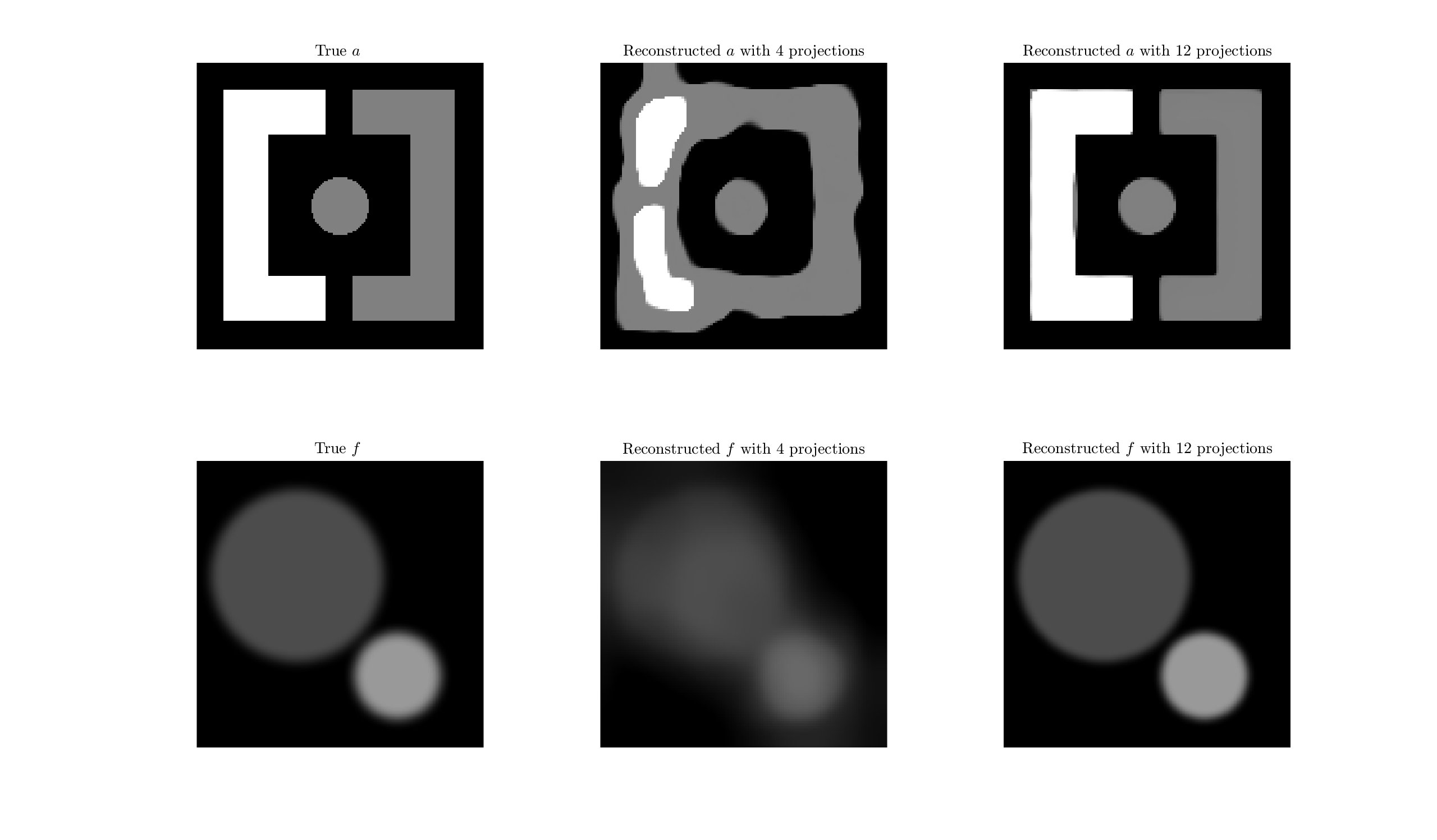
Figure 5 shows the effect of the number of projections on reconstruction quality. Here the phantom is made up of 3 regions with . The left column shows the true phantoms for and . The middle column is an optimized reconstruction using 6 projections with and . The right column shows an optimized reconstruction using 12 projections with and . In both reconstructions for we obtain multi-bang solutions. The middle column shows a poor recovery of the structure of and . The recovered has a lot of misclassification and has been unable to separate the regions. The inaccuracies in have an impact on the recovery of , with the outer most regions of being poorly recovered. The rightmost column is a very good recovery of both and , with just a small section on the left bracket being misclassified. The matching is also very well recovered. Although the smoothed TV regularization removes cross talk artefacts it is important not to use too large as this removes the continuous nature of at the edges. We also remark that there is no significant improvement in the quality of the reconstruction if we increase the number of projections further.

Figure 6 shows a plot of the proportion of pixels taking admissible values against outer iteration number (that is in Algorithm 1) for the rightmost reconstruction of in Figure 5. The initial guess is constant at 0, which is why the initial proportion is 1. The proportion increases monotonically after about 20 iterations with some large jumps before this point. These typically line up with being either increased or decreased in the inner iterations. This graph is typical for reconstructions presented here and suggests that another suitable stopping criteria would be to terminate after a certain proportion of admissible values is reached. Typically a convergent reconstruction has a multi-bang proportion of over 0.95 by the time the algorithm is terminated by the step size tolerances.

Figure 7 shows the effect of shrinking the size of the support of on reconstruction. This is linked to the proof of uniqueness from Theorems 1 and 2, where we require to be non-zero on a sufficient number of rays tangent to the jumps in . Here the true is a multi-bang version of the Shepp-Logan phantom, with admissable set . The step sizes are and and regularization parameters are and for each reconstruction. The top row shows reconstructions of with fixed and known true in the bottom row. The reconstruction algorithm here is then performed by simply performing one update for . The rightmost reconstruction captures the shape and classifies almost all pixels correctly; most importantly it captures the smallest regions well. Note here that as in Theorem 1 and 2 has a larger support than . It is possible to obtain reconstructions similar to that of the rightmost recovery for which have a slightly smaller support than . The 2nd column from the right also has a decent shape recovery but has lost some of the finer features such as the ellipses at the bottom. The 2nd column from the left does a poor job of the recovery of with very few pixels correctly classified as . The high valued outer ellipse is lost and all the finer details are missing. This is a similar effect to reducing the number of projections, which could be expected as reducing leads to fewer rays contributing data per projection. We can however still see some detail outside of the support of , this is due to TV being able to fill in the gaps and extend our visibility. The angled straight edges in the reconstruction are related to the angles of the projections in the data set.

The final numerical result we present in Figure 8 is obtained using an image of a walnut reconstructed from CT data by the Finnish Inverse Problems Society [finnish] as the attenuation map. The walnut phantom for is binary and so . Here the step sizes are and and the regularization parameters are and . The left hand column is the true and and the right hand column the reconstruction. In general the larger structures of are recovered but the finer details are lost. This is still true even if the number of projections is upped significantly. This is in part due to the detail being compressed going from 340 by 340 to 200 by 200 pixels and the TV regularizer eliminating the smallest non-zero regions. The larger sections are well-recovered and the outermost boundary is very well classified. The reconstruction for is again good with the areas towards the boundaries being the areas most affected by the errors in . There are no cross-talk artefacts present, even with the more complicated .
5 Conclusion
In this paper we have presented and proved two theorems on the identification problem for SPECT involving multi-bang attenuation. In particular, for nicely multi-bang and non-negative with sufficiently large support we have shown uniqueness of joint recovery for the AtRT. The method of proof for these theorems gives possible methods to produce similar results with further relaxed conditions on and , and we intend to investigate this in future work.
On the numerical side, we have formulated a variational problem including a weakly convex version of the convex multi-bang regularizer[MB, MBorig] and a smoothed total variation, and presented an algorithm for simultaneous recovery of and from the resulting variational problem (26). Using an alternating direction approach for non-convex objective functions [alternating] coupled with ADMM[addm] we are able to successfully solve these variational problems. The addition of a joint multi-bang and total variation regularizer has produced good results for joint recovery with projection numbers similar to those used in the X-Ray recovery case when the image is known to have only a finite number of values [chenrays, limrays]. The apparent convergence of the algorithm even in the case in all cases we have investigated, and also independent of the smoothing parameter for the total variation presents theoretical questions for future work. Also, even though the variational problems on which our method is based are non-convex, our algorithm consistently converges to a reasonable approximation for the correct solution. This suggests we may actually be finding the global minimiser, or be getting close to the global minimiser, and there is potential for future research investigating whether this is indeed correct.
Finally, the numerical examples shown in Figure 7 indicate that we are able to obtain good recovery for even when the support of is smaller than required in our theoretical results. We suspect that the total variation may be playing a role in filling in the boundaries of regions of constant , and would like to investigate this further as well.
Numerical results from joint reconstruction/Multibang˙Holman˙Richardson.bbl