跳到论文正文
W Papers独立论文阅读器 arXiv:2001.04080 论文正文 计算阅读时间 · 0%
引用这篇论文根据当前论文元数据生成,正式投稿前建议核对。


License: arXiv.org perpetual non-exclusive license
arXiv:2001.04080v1 [math.SP] 13 Jan 2020

Perturbation analysis for the linear operator equation using pseudospectrum and condition pseudospectrum

Krishna Kumar. G Address: Department of Mathematics, Baby John Memorial Government College Chavara, Kollam, Kerala, India, 691583. Email address: krishna.math@gmail.com
Abstract.

In this article, we consider the linear operator equation A​x−z​x=yAx-zx=y in a Banach space. The relative perturbation of the solution xx corresponding to the perturbation of yy, the perturbation of AA and the perturbation of both A,yA,y are characterized from the pseudospectrum and the condition pseudospectrum of AA. Certain examples are given to illustrate the results. A relation between the pseudospectrum and the condition pseudospectrum of an operator are established. The distance to instability and the distance to singularity of an operator are also found from the condition pseudospectrum of the operator.

Key words and phrases: 
pseudospectrum, condition pseudospectrum, perturbation, relative error, instability
2010 Mathematics Subject Classification
Primary 47A55; Secondary 15A09, 47A10, 47A30, 47A50

1. Introduction

Throughout this article XX denotes a complex Banach space and B​L​(X)BL(X) is the Banach algebra of all bounded linear operators on XX. Define ℐ:={z​I:z∈ℂ}\mathcal{I}:=\{zI:z\in\mathbb{C}\}, where II is the identity operator in B​L​(X)BL(X).

Definition 1.1.

Let A∈B​L​(X)A\in BL(X). The spectrum of AA is denoted by σ⁡(A)\sigma(A) and is defined as

σ(A):={z∈ℂ:A−zIis not invertible}.\sigma(A):=\{z\in\mathbb{C}:A-zI\ \ \mbox{is not invertible}\}.

The spectrum of an operator in B​L​(X)BL(X) is generalized in many ways for various applications. The pseudospectrum and the condition pseudospectrum are two important generalizations of the spectrum of an operator.

Definition 1.2.

Let A∈B​L​(X)A\in BL(X) and ϵ>0\epsilon>0. The ϵ\epsilon-pseudospectrum of AA is denoted by Λϵ​(A)\Lambda_{\epsilon}(A) and is defined as

Λϵ​(A):=σ⁡(A)∪{z∈ℂ:‖(A−z​I)−1‖≥ϵ−1}.\Lambda_{\epsilon}(A):=\sigma(A)\cup\left\{z\in\mathbb{C}:\|(A-zI)^{-1}\|\geq\epsilon^{-1}\right\}.

Hence σ⁡(A)⊆Λϵ​(A)\sigma(A)\subseteq\Lambda_{\epsilon}(A) for each ϵ>0\epsilon>0 and ⋂ϵ>0Λϵ​(A)=σ⁡(A)\displaystyle\bigcap_{\epsilon>0}\Lambda_{\epsilon}(A)=\sigma(A). For more properties and various applications of the pseudospectrum one may refer to [9].

Definition 1.3.

Let A∈B​L​(X)A\in BL(X) and 0<ϵ<10<\epsilon<1. The ϵ\epsilon-condition pseudospectrum of AA is denoted by σϵ​(A)\sigma_{\epsilon}(A) and is defined as

σϵ​(A):=σ⁡(A)∪{z∈ℂ:‖A−z​I‖​‖(A−z​I)−1‖≥ϵ−1}.\sigma_{\epsilon}(A):=\sigma(A)\cup\left\{z\in\mathbb{C}:\|A-zI\|\|(A-zI)^{-1}\|\geq\epsilon^{-1}\right\}.

Hence σ⁡(A)⊆σϵ​(A)\sigma(A)\subseteq\sigma_{\epsilon}(A) for each 0<ϵ<10<\epsilon<1, ⋂0<ϵ<1σϵ​(A)=σ⁡(A)\displaystyle\bigcap_{0<\epsilon<1}\sigma_{\epsilon}(A)=\sigma(A) and σ1​(A)=ℂ\sigma_{1}(A)=\mathbb{C}. The condition pseudospectrum was introduced in [6] and in the same article it is called condition spectrum. Compare to several other generalizations of the spectrum, the condition pseudospectrum is proved to be algebraically close to the spectrum. Hence the condition pseudospectrum is useful to study the perturbation analysis of operators of B​L​(X)BL(X). For more properties of the condition pseudospectrum one may refer to [1, 3, 4, 5, 6, 7].

Let A∈B​L​(X)A\in BL(X). Consider the linear operator equation A​x−z​x=yAx-zx=y where x,y∈Xx,y\in X and z∈ℂz\in\mathbb{C}. The purpose of the article is to characterize the perturbation of the solution xx corresponding to the following perturbations from the pseudospectrum and the condition pseudospectrum of AA.

  1. (1)

    the perturbation of yy

  2. (2)

    the perturbation of AA

  3. (3)

    the perturbation of both AA and yy

The following is an outline of the article. In section 2, we consider certain linear operator equations A​x−z​x=yAx-zx=y to illustrate that the perturbation of the solution xx corresponding to the perturbation of yy, perturbation of AA and perturbation of both A,yA,y depends on the pseudospectrum and the condition pseudospectrum of the operator AA. In section 3, an upper bound and lower bound is found for the relative perturbation of the solution xx corresponding to the relative perturbation of yy from the condition pseudospectrum of AA (Theorem 3.1). An upper bound is found for the relative perturbation of the solution xx corresponding to the relative perturbation of the operator AA from the pseudospectrum of AA (Theorem 3.3) and the condition pseudospectrum of AA (Theorem 3.5). An upper bound is found for the relative perturbation of the solution xx corresponding to the relative perturbation of both AA and yy from the condition pseudospectrum of AA ( Theorem 3.7). Certain examples are also given to illustrate the results. In section 4, a relation connecting the pseudospectrum and the condition pseudospectrum of an operator in B​L​(X)BL(X) is given as set inclusions. The distance to instability of an operator in B​L​(X)BL(X) is also characterized from the condition pseudospectrum of the operator. In section 5, the distance to singularity of an invertible operator in B​L​(X)BL(X) is characterized from the condition pseudospectrum of the operator.

2. Preliminaries

Let A∈B​L​(X)A\in BL(X). Consider the the linear operator equation

A​x−z​x=yAx-zx=y

where x,y∈Xx,y\in X and z∈ℂz\in\mathbb{C}. The following example finds the perturbation of the solution xx corresponding to various perturbations of yy. We claim that the perturbation of the solution depends on the quantity ‖A−z​I‖​‖(A−z​I)−1‖\|A-zI\|\|(A-zI)^{-1}\| and hence the perturbation of the solution may characterized from the condition pseudospectrum of the operator AA.

Example 2.1.

Consider the linear systems defined by

A​x1−x1=yandB​x2−x2=yAx_{1}-x_{1}=y\ \ \textnormal{and}\ \ Bx_{2}-x_{2}=y

where A=[1.1002]A=\begin{bmatrix}1.1&0\\ 0&2\end{bmatrix}, B=[1.11002]B=\begin{bmatrix}1.1&10\\ 0&2\end{bmatrix} and y=[11]y=\begin{bmatrix}1\\ 1\end{bmatrix}. Let δ​y\delta y be a small perturbation on yy and δ​x1,δ​x2\delta x_{1},\delta x_{2} be the corresponding perturbations of the solution x1,x2x_{1},x_{2} respectively. Then

(A−I)​(x1+δ​x1)=y+δ​yand(B−I)​(x2+δ​x2)=y+δ​y.(A-I)(x_{1}+\delta x_{1})=y+\delta y\ \ \textnormal{and}\ \ (B-I)(x_{2}+\delta x_{2})=y+\delta y.

The following table gives the perturbations of the solutions for various values of δ​y\delta y.

δ​y\delta y δ​x1\delta x_{1} ‖δ​x1‖‖x1‖\frac{\|\delta x_{1}\|}{\|x_{1}\|} δ​x2\delta x_{2} ‖δ​x2‖‖x2‖\frac{\|\delta x_{2}\|}{\|x_{2}\|}
[0.01,0.01]T[0.01,0.01]^{T} [0.1,0.01]T[0.1,0.01]^{T} 0.01 [−0.9,0.01]T[-0.9,0.01]^{T} 0.01
[0.01,0.02]T[0.01,0.02]^{T} [0.1,0.02]T[0.1,0.02]^{T} 0.0101474 [−1.9,0.02]T[-1.9,0.02]^{T} 0.0211109
[0.02,0.01]T[0.02,0.01]^{T} [0.2,0.01]T[0.2,0.01]^{T} 0.0199256 [−0.8,0.01]T[-0.8,0.01]^{T} 0.008889
[0.02,0.02]T[0.02,0.02]^{T} [0.2,0.02]T[0.2,0.02]^{T} 0.02 [−1.8,0.02]T[-1.8,0.02]^{T} 0.02
[0.03,−0.03]T[0.03,-0.03]^{T} [0.3,−0.03]T[0.3,-0.03]^{T} 0.03 [3.3,−0.03]T[3.3,-0.03]^{T} 0.0366659
[0.04,−0.04]T[0.04,-0.04]^{T} [0.4,−0.04]T[0.4,-0.04]^{T} 0.04 [4.4,−0.04]T[4.4,-0.04]^{T} 0.0488879
[0.05,−0.05]T[0.05,-0.05]^{T} [0.5,−0.05]T[0.5,-0.05]^{T} 0.05 [5.5,−0.05]T[5.5,-0.05]^{T} 0.0611098
[0.06,−0.06]T[0.06,-0.06]^{T} [0.6,−0.06]T[0.6,-0.06]^{T} 0.06 [6.6,−0.06]T[6.6,-0.06]^{T} 0.0733318
Refer to caption Refer to caption
Figure 1.

In Figure 1, the ϵ\epsilon-condition pseudospectrum of AA and BB are found for ϵ=0.1,0.15,0.2\epsilon=0.1,0.15,0.2 and 0.250.25. For z∈ℂz\in\mathbb{C} and A∈B​L​(X)A\in BL(X) define

κ⁡(z,A):=sup{0<ϵ<1:z∉σϵ​(A)}.\kappa(z,A):=\sup\{0<\epsilon<1:z\notin\sigma_{\epsilon}(A)\}.

Then κ⁡(z,B)≤κ⁡(z,A)\kappa(z,B)\leq\kappa(z,A) for every z∈ℂz\in\mathbb{C} and σϵ​(A)⊆σϵ​(B)\sigma_{\epsilon}(A)\subseteq\sigma_{\epsilon}(B) for each 0<ϵ<10<\epsilon<1. The following example finds the perturbation of the solution xx corresponding to various perturbations of AA. We claim that the perturbation of the solution depends on the quantity ‖(A−z​I)−1‖\|(A-zI)^{-1}\| and hence the perturbation of the solution may characterized from the pseudospectrum of the operator AA.

Example 2.2.

Consider the linear systems defined by

A​x1−2​x1=yandB​x2−2​x2=yAx_{1}-2x_{1}=y\ \ \textnormal{and}\ \ Bx_{2}-2x_{2}=y

where A=[10−102.11003]A=\begin{bmatrix}1&0&-1\\ 0&2.1&1\\ 0&0&3\end{bmatrix}, B=[1101002.110003]B=\begin{bmatrix}1&10&10\\ 0&2.1&10\\ 0&0&3\end{bmatrix} and y=[111]y=\begin{bmatrix}1\\ 1\\ 1\end{bmatrix}. Let Δ​A,Δ​B\Delta A,\Delta B be small perturbations on A,BA,B and δ​x1,δ​x2\delta x_{1},\delta x_{2} be the corresponding perturbations of the solution x1,x2x_{1},x_{2} respectively. Then

(A−2​I+Δ​A)​(x1+δ​x1)=yand(B−2​I+Δ​B)​(x2+δ​x2)=y.(A-2I+\Delta A)(x_{1}+\delta x_{1})=y\ \ \textnormal{and}\ \ (B-2I+\Delta B)(x_{2}+\delta x_{2})=y.

The following table gives the perturbation of the solution xx corresponding to various perturbations of AA and BB. Choose Δ​A=Δ​B=[ϵ1000ϵ20000]\Delta A=\Delta B=\begin{bmatrix}\epsilon_{1}&0&0\\ 0&\epsilon_{2}&0\\ 0&0&0\end{bmatrix}.

Δ​A=Δ​B\Delta A=\Delta B δ​x1\delta x_{1} ‖δ​x1‖‖x1‖\frac{\|\delta x_{1}\|}{\|x_{1}\|} δ​x2\delta x_{2} ‖δ​x2‖‖x2‖\frac{\|\delta x_{2}\|}{\|x_{2}\|}
ϵ1=0.01,ϵ2=0.01\epsilon_{1}=0.01,\epsilon_{2}=0.01 [−0.02020202,0,0]T[-0.02020202,0,0]^{T} 0.0090346 [73.64463,8.18182,0]T[73.64463,8.18182,0]^{T} 0.0827413
ϵ1=0.02,ϵ2=0.02\epsilon_{1}=0.02,\epsilon_{2}=0.02 [−0.04081633,0,0]T[-0.04081633,0,0]^{T} 0.0182536 [134.87755,15,0]T[134.87755,15,0]^{T} 0.1515397
ϵ1=0.03,ϵ2=0.03\epsilon_{1}=0.03,\epsilon_{2}=0.03 [−0.06185567,0,0]T[-0.06185567,0,0]^{T} 0.0276626 [186.55908,20.76923,0]T[186.55908,20.76923,0]^{T} 0.2096085
ϵ1=0.04,ϵ2=0.04\epsilon_{1}=0.04,\epsilon_{2}=0.04 [−0.08333333,0,0]T[-0.08333333,0,0]^{T} 0.0372677 [230.73214,25.71428,0]T[230.73214,25.71428,0]^{T} 0.2592425
ϵ1=0.05,ϵ2=0.05\epsilon_{1}=0.05,\epsilon_{2}=0.05 [−0.10526316,0,0]T[-0.10526316,0,0]^{T} 0.0470751 [268.89473,30,0]T[268.89473,30,0]^{T} 0.302125
ϵ1=0.06,ϵ2=0.06\epsilon_{1}=0.06,\epsilon_{2}=0.06 [−0.12765957,0,0]T[-0.12765957,0,0]^{T} 0.0570910 [302.170212,33.75,0]T[302.170212,33.75,0]^{T} 0.339517
ϵ1=0.07,ϵ2=0.07\epsilon_{1}=0.07,\epsilon_{2}=0.07 [−0.15053763,0,0]T[-0.15053763,0,0]^{T} 0.0673224 [331.41745,37.05882,0]T[331.41745,37.05882,0]^{T} 0.3723843
Refer to caption Refer to caption
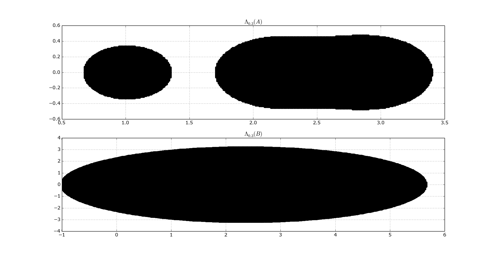
Figure 2.

In Figure 2, the ϵ\epsilon-pseudospectrum of AA and BB are found for ϵ=0.2,0.3,0.4\epsilon=0.2,0.3,0.4 and 0.50.5. For z∈ℂz\in\mathbb{C} and A∈B​L​(X)A\in BL(X) define

κ1​(z,A):=sup{ϵ>0:z∉Λϵ​(A)}.\kappa_{1}(z,A):=\sup\{\epsilon>0:z\notin\Lambda_{\epsilon}(A)\}.

Then κ1​(z,B)≤κ1​(z,A)\kappa_{1}(z,B)\leq\kappa_{1}(z,A) for every z∈ℂz\in\mathbb{C} and Λϵ​(A)⊆Λϵ​(B)\Lambda_{\epsilon}(A)\subseteq\Lambda_{\epsilon}(B) for each ϵ>0\epsilon>0. The following example finds the perturbation of the solution xx corresponding to various perturbations of A,yA,y. We claim that the perturbation of the solution depends on the quantity ‖A−z​I‖​‖(A−z​I)−1‖\|A-zI\|\|(A-zI)^{-1}\| and hence the perturbation of the solution may characterized from the condition pseudospectrum of the operator AA.

Example 2.3.

Consider the linear systems defined by

A​x1−3​x1=yandB​x2−3​x2=yAx_{1}-3x_{1}=y\ \ \textnormal{and}\ \ Bx_{2}-3x_{2}=y

where A=[10−1021003.1]A=\begin{bmatrix}1&0&-1\\ 0&2&1\\ 0&0&3.1\end{bmatrix}, B=[110100210003.1]B=\begin{bmatrix}1&10&10\\ 0&2&10\\ 0&0&3.1\end{bmatrix} and y=[111]y=\begin{bmatrix}1\\ 1\\ 1\end{bmatrix}. Let Δ​A,Δ​B\Delta A,\Delta B be a small perturbations on A,BA,B respectively and δ​y\delta y be a small perturbation on yy. Further let δ​x1,δ​x2\delta x_{1},\delta x_{2} be the corresponding perturbations of the solution x1,x2x_{1},x_{2}. Then

(A−3​I+Δ​A)​(x1+δ​x1)=y+δ​yand(B−3​I+Δ​B)​(x2+δ​x2)=y+δ​y.(A-3I+\Delta A)(x_{1}+\delta x_{1})=y+\delta y\ \ \textnormal{and}\ \ (B-3I+\Delta B)(x_{2}+\delta x_{2})=y+\delta y.

The following table gives the perturbation of the solution xx corresponding to various perturbations of A,BA,B and δ​y\delta y. Choose Δ​A=Δ​B=[0000ϵ1000ϵ2]\Delta A=\Delta B=\begin{bmatrix}0&0&0\\ 0&\epsilon_{1}&0\\ 0&0&\epsilon_{2}\end{bmatrix}.

Δ​A=Δ​B\Delta A=\Delta B δ​y\delta y δ​x1\delta x_{1} δ​x2\delta x_{2}
ϵ1=0.01,ϵ2=0.01\epsilon_{1}=0.01,\epsilon_{2}=0.01 [0.01,0.01,0.01]T[0.01,0.01,0.01]^{T} [0.404,−0.745,−0.818]T[0.404,-0.745,-0.818]^{T} [−40.468,−7.274,−0.818]T[-40.468,-7.274,-0.818]^{T}
ϵ1=0.02,ϵ2=0.02\epsilon_{1}=0.02,\epsilon_{2}=0.02 [0.02,0.02,0.02]T[0.02,0.02,0.02]^{T} [0.74,−1.367,−1.5]T[0.74,-1.367,-1.5]^{T} [−74.040,−13.306,−1.5]T[-74.040,-13.306,-1.5]^{T}
ϵ1=0.03,ϵ2=0.03\epsilon_{1}=0.03,\epsilon_{2}=0.03 [0.03,0.03,0.03]T[0.03,0.03,0.03]^{T} [1.023,−1.893,−2.076]T[1.023,-1.893,-2.076]^{T} [−102.302,−18.380,−2.076]T[-102.302,-18.380,-2.076]^{T}
ϵ1=0.04,ϵ2=0.04\epsilon_{1}=0.04,\epsilon_{2}=0.04 [0.04,0.04,0.04]T[0.04,0.04,0.04]^{T} [1.265,−2.345,−2.571]T[1.265,-2.345,-2.571]^{T} [−126.389,−22.702,−2.571]T[-126.389,-22.702,-2.571]^{T}
ϵ1=0.05,ϵ2=0.05\epsilon_{1}=0.05,\epsilon_{2}=0.05 [0.05,0.05,0.05]T[0.05,0.05,0.05]^{T} [1.475,−2.736,−3]T[1.475,-2.736,-3]^{T} [−147.130,−26.421,−3]T[-147.130,-26.421,-3]^{T}
ϵ1=0.06,ϵ2=0.06\epsilon_{1}=0.06,\epsilon_{2}=0.06 [0.06,0.06,0.06]T[0.06,0.06,0.06]^{T} [1.657,−3.079,−3.375]T[1.657,-3.079,-3.375]^{T} [−165.149,−29.648,−3.375]T[-165.149,-29.648,-3.375]^{T}
ϵ1=0.07,ϵ2=0.07\epsilon_{1}=0.07,\epsilon_{2}=0.07 [0.07,0.07,0.07]T[0.07,0.07,0.07]^{T} [1.817,−3.382,−3.705]T[1.817,-3.382,-3.705]^{T} [−180.923,−32.471,−3.705]T[-180.923,-32.471,-3.705]^{T}
Refer to caption Refer to caption
Figure 3.

In Figure 3, the ϵ\epsilon-condition pseudospectrum of AA and BB are found for ϵ=0.1,0.15,0.2\epsilon=0.1,0.15,0.2 and 0.250.25. Then κ⁡(z,B)≤κ⁡(z,A)\kappa(z,B)\leq\kappa(z,A) for every z∈ℂz\in\mathbb{C} and σϵ​(A)⊆σϵ​(B)\sigma_{\epsilon}(A)\subseteq\sigma_{\epsilon}(B) for each 0<ϵ<10<\epsilon<1.

3. The stability of linear operator equations

3.1. Perturbation of yy

Let A∈B​L​(X)A\in BL(X) and A​x−z​x=yAx-zx=y where x,y∈Xx,y\in X and z∈ℂz\in\mathbb{C}. The following theorem finds an upper bound and lower bound for the relative perturbations of the solution xx from the condition pseudospectrum of AA.

Theorem 3.1.

Let A∈B​L​(X)A\in BL(X) and A​x−z​x=yAx-zx=y where x,y∈Xx,y\in X and z∉σ⁡(A)z\notin\sigma(A). Further let δ​x\delta x be the perturbation of the solution xx corresponding to a perturbation δ​y\delta y of yy. Then

κ⁡(z,A)​‖δ​y‖‖y‖≤‖δ​x‖‖x‖≤1κ⁡(z,A)​‖δ​y‖‖y‖\kappa(z,A)\,\frac{\|\delta y\|}{\|y\|}\leq\frac{\|\delta x\|}{\|x\|}\leq\frac{1}{\kappa(z,A)}\frac{\|\delta y\|}{\|y\|}

where κ⁡(z,A):=sup{0<ϵ<1:z∉σϵ​(A)}.\displaystyle\kappa(z,A):=\sup\{0<\epsilon<1:z\notin\sigma_{\epsilon}(A)\}.

Proof.

We have

(A−z​I)​(x+δ​x)=y+δ​y.(A-zI)(x+\delta x)=y+\delta y.

Since z∉σ⁡(A)z\notin\sigma(A),

(3.1) ‖x‖≤‖(A−z​I)−1‖​‖y‖and‖y‖≤‖A−z​I‖​‖x‖.\displaystyle\|x\|\leq\|(A-zI)^{-1}\|\|y\|\ \ \mbox{and}\ \ \|y\|\leq\|A-zI\|\|x\|.

Also

(3.2) ‖δ​y‖≤‖A−z​I‖​‖δ​x‖and‖δ​x‖≤‖(A−z​I)−1‖​‖δ​y‖.\displaystyle\|\delta y\|\leq\|A-zI\|\|\delta x\|\ \ \mbox{and}\ \ \|\delta x\|\leq\|(A-zI)^{-1}\|\|\delta y\|.

From (3.1) and (3.2) it follows that

1‖(A−z​I)‖​‖(A−z​I)−1‖​‖δ​y‖‖y‖≤‖δ​x‖‖x‖≤‖A−z​I‖​‖(A−z​I)−1‖​‖δ​y‖‖y‖.\frac{1}{\|(A-zI)\|\|(A-zI)^{-1}\|}\frac{\|\delta y\|}{\|y\|}\leq\frac{\|\delta x\|}{\|x\|}\leq\|A-zI\|\|(A-zI)^{-1}\|\frac{\|\delta y\|}{\|y\|}.

If z∉σϵ​(A)z\notin\sigma_{\epsilon}(A) for some 0<ϵ<10<\epsilon<1, then

ϵ​‖δ​y‖‖y‖<‖δ​x‖‖x‖<1ϵ​‖δ​y‖‖y‖.\epsilon\,\frac{\|\delta y\|}{\|y\|}<\frac{\|\delta x\|}{\|x\|}<\frac{1}{\epsilon}\frac{\|\delta y\|}{\|y\|}.

Define κ⁡(z,A):=sup{0<ϵ<1:z∉σϵ​(A)}.\displaystyle\kappa(z,A):=\sup\{0<\epsilon<1:z\notin\sigma_{\epsilon}(A)\}. Then

κ⁡(z,A)​‖δ​y‖‖y‖≤‖δ​x‖‖x‖≤1κ⁡(z,A)​‖δ​y‖‖y‖.\kappa(z,A)\,\frac{\|\delta y\|}{\|y\|}\leq\frac{\|\delta x\|}{\|x\|}\leq\frac{1}{\kappa(z,A)}\frac{\|\delta y\|}{\|y\|}.

∎

Example 3.2.

Consider the operator equation A​x−z​x=yAx-zx=y defined by

A=[011401⋱⋱⋱1401140]10×10​andy=[.1111]10×1.A=\begin{bmatrix}0&1&&&\\ \frac{1}{4}&0&1&&\\ &\ddots&\ddots&\ddots&\\ &&\frac{1}{4}&0&1\\ &&&\frac{1}{4}&0\\ \end{bmatrix}_{10\times 10}\mbox{and}\ \ \ \ y=\begin{bmatrix}.1\\ 1\\ \vdots\\ 1\\ 1\end{bmatrix}_{10\times 1}.

The following table gives the relative perturbation of the solution xx for various values of zz and for δ​y=[0.1000000000]T\delta y=\begin{bmatrix}0.1&0&0&0&0&0&0&0&0&0\end{bmatrix}^{T}. The table also gives the upper bound and lower bound for the relative perturbation of the solution found from the condition pseudospectrum of AA.

zz ‖δ​x‖‖x‖\frac{\|\delta x\|}{\|x\|} κ⁡(z,A)\kappa(z,A) κ⁡(z,A)​‖δ​y‖‖y‖\kappa(z,A)\frac{\|\delta y\|}{\|y\|} 1κ⁡(z,A)​‖δ​y‖‖y‖\frac{1}{\kappa(z,A)}\frac{\|\delta y\|}{\|y\|}
22 0.01451478 0.25562528 0.00808358 0.12370754
2+i2+i 0.01916041 0.34480349 0.01090364 0.09171245
3−i3-i 0.02157139 0.22394260 0.00708168 0.14120929
1−i1-i 0.02192375 0.22394260 0.00708168 0.14120929
2−i2-i 0.01916041 0.34480349 0.01090364 0.09171245
3+3​i3+3i 0.02634769 0.62518073 0.01976995 0.05058181
4​i4i 0.03238426 0.69642891 0.02202301 0.04540704

3.2. Perturbation of AA

Let A∈B​L​(X)A\in BL(X) and A​x−z​x=yAx-zx=y where x,y∈Xx,y\in X and z∈ℂz\in\mathbb{C}. The following theorem finds an upper bound for ‖δ​x‖‖x‖,‖δ​x‖‖x+δ​x‖\frac{\|\delta x\|}{\|x\|},\frac{\|\delta x\|}{\|x+\delta x\|} from the pseudospectrum of A+Δ​AA+\Delta A, AA respectively.

Theorem 3.3.

Let A∈B​L​(X)A\in BL(X) and A​x−z​x=yAx-zx=y where x,y∈Xx,y\in X and z∉σ⁡(A)z\notin\sigma(A). Further let δ​x\delta x be the perturbation of the solution xx corresponding to the perturbation Δ​A\Delta A of AA. Then

  1. (1)

    ‖δ​x‖‖x‖≤‖Δ​A‖κ1​(z,A+Δ​A)\frac{\|\delta x\|}{\|x\|}\leq\frac{\|\Delta A\|}{\kappa_{1}(z,A+\Delta A)}.

  2. (2)

    ‖δ​x‖‖x+δ​x‖≤‖Δ​A‖κ1​(z,A)\frac{\|\delta x\|}{\|x+\delta x\|}\leq\frac{\|\Delta A\|}{\kappa_{1}(z,A)}.

where κ1​(z,A):=sup{ϵ>0:z∉Λϵ​(A)}.\displaystyle\kappa_{1}(z,A):=\sup\{\epsilon>0:z\notin\Lambda_{\epsilon}(A)\}.

Proof.
  1. (1)

    We have (A−z​I+Δ​A)​(x+δ​x)=y.(A-zI+\Delta A)(x+\delta x)=y. Then

    (A−z​I)​δ​x+Δ​A​(x+δ​x)=0.(A-zI)\delta x+\Delta A(x+\delta x)=0.

    If z∉Λϵ​(A+Δ​A)z\notin\Lambda_{\epsilon}(A+\Delta A) for some ϵ>0\epsilon>0. Then ‖δ​x‖≤‖(A+Δ​A−z​I)−1‖​‖Δ​A‖​‖x‖\|\delta x\|\leq\|(A+\Delta A-zI)^{-1}\|\|\Delta A\|\|x\| and ‖δ​x‖‖x‖<‖Δ​A‖ϵ.\frac{\|\delta x\|}{\|x\|}<\frac{\|\Delta A\|}{\epsilon}. Define κ1​(z,A+Δ​A):=sup{ϵ>0:z∉Λϵ​(A+Δ​A)}.\displaystyle\kappa_{1}(z,A+\Delta A):=\sup\{\epsilon>0:z\notin\Lambda_{\epsilon}(A+\Delta A)\}. Then

    ‖δ​x‖‖x‖≤‖Δ​A‖κ1​(z,A+Δ​A).\frac{\|\delta x\|}{\|x\|}\leq\frac{\|\Delta A\|}{\kappa_{1}(z,A+\Delta A)}.
  2. (2)

    If z∉Λϵ​(A)z\notin\Lambda_{\epsilon}(A) for some ϵ>0\epsilon>0. Then ‖δ​x‖≤‖(A−z​I)−1‖​‖Δ​A‖​‖x+δ​x‖\|\delta x\|\leq\|(A-zI)^{-1}\|\|\Delta A\|\|x+\delta x\| and ‖δ​x‖‖x+δ​x‖<‖Δ​A‖ϵ.\frac{\|\delta x\|}{\|x+\delta x\|}<\frac{\|\Delta A\|}{\epsilon}. Define κ1​(z,A):=sup{ϵ>0:z∉Λϵ​(A)}.\displaystyle\kappa_{1}(z,A):=\sup\{\epsilon>0:z\notin\Lambda_{\epsilon}(A)\}. Then

    ‖δ​x‖‖x+δ​x‖≤‖Δ​A‖κ1​(z,A).\frac{\|\delta x\|}{\|x+\delta x\|}\leq\frac{\|\Delta A\|}{\kappa_{1}(z,A)}.

∎

Lemma 3.4.

Let A∈B​L​(X)A\in BL(X). Then for every z∈ℂz\in\mathbb{C}

sup{‖A−λ​I‖:λ∈σ⁡(A)}≤‖A−z​I‖.\sup\{\|A-\lambda I\|:\lambda\in\sigma(A)\}\leq\|A-zI\|.
Proof.

If λ∈σ⁡(A)\lambda\in\sigma(A) and z∈ℂz\in\mathbb{C}. Then λ−z∈σ⁡(A−z​I)\lambda-z\in\sigma(A-zI) and |λ−z|≤‖A−z​I‖|\lambda-z|\leq\|A-zI\|. Also

‖A−λ​I‖=‖A−z​I+z​I−λ​I‖≤‖A−z​I‖+|λ−z|≤2​‖A−z​I‖.\|A-\lambda I\|=\|A-zI+zI-\lambda I\|\leq\|A-zI\|+|\lambda-z|\leq 2\|A-zI\|.

∎

The following theorem finds an upper bound for ‖δ​x‖‖x‖,‖δ​x‖‖x+δ​x‖\frac{\|\delta x\|}{\|x\|},\frac{\|\delta x\|}{\|x+\delta x\|} from the condition pseudospectrum of A+Δ​A,AA+\Delta A,A respectively.

Theorem 3.5.

Let A∈B​L​(X)A\in BL(X) and A​x−z​x=yAx-zx=y where x,y∈Xx,y\in X and z∉σ⁡(A)z\notin\sigma(A). Further let δ​x\delta x be a perturbation of the solution xx corresponding to the perturbation Δ​A\Delta A of AA. Define κ⁡(z,A):=sup{0<ϵ<1:z∉σϵ​(A)}.\displaystyle\kappa(z,A):=\sup\{0<\epsilon<1:z\notin\sigma_{\epsilon}(A)\}. Then

  1. (1)

    ‖δ​x‖‖x‖≤2​‖Δ​A‖M1​κ​(z,A+Δ​A)\frac{\|\delta x\|}{\|x\|}\leq\frac{2\|\Delta A\|}{M_{1}\,\kappa(z,A+\Delta A)} where M1:=sup{‖A+Δ​A−λ​I‖:λ∈σ⁡(A+Δ​A)}M_{1}:=\sup\{\|A+\Delta A-\lambda I\|:\lambda\in\sigma(A+\Delta A)\}.

  2. (2)

    ‖δ​x‖‖x+δ​x‖≤2​‖Δ​A‖M2​κ​(z,A)\frac{\|\delta x\|}{\|x+\delta x\|}\leq\frac{2\|\Delta A\|}{M_{2}\,\kappa(z,A)} where M2:=sup{‖A−λ​I‖:λ∈σ⁡(A)}M_{2}:=\sup\{\|A-\lambda I\|:\lambda\in\sigma(A)\}.

Proof.
  1. (1)

    We have (A−z​I+Δ​A)​(x+δ​x)=y(A-zI+\Delta A)(x+\delta x)=y and

    (A−z​I)​δ​x+Δ​A​(x+δ​x)=0.(A-zI)\delta x+\Delta A(x+\delta x)=0.

    If z∉σϵ​(A+Δ​A)z\notin\sigma_{\epsilon}(A+\Delta A) for some 0<ϵ<10<\epsilon<1. Then

    ‖δ​x‖≤‖A+Δ​A−z​I‖​‖(A+Δ​A−z​I)−1‖​‖Δ​A‖​‖x‖‖A+Δ​A−z​I‖.\|\delta x\|\leq\frac{\|A+\Delta A-zI\|\|(A+\Delta A-zI)^{-1}\|\|\Delta A\|\|x\|}{\|A+\Delta A-zI\|}.

    From Lemma 3.4,

    ‖δ​x‖‖x‖≤2​‖Δ​A‖M1​ϵ\frac{\|\delta x\|}{\|x\|}\leq\frac{2\|\Delta A\|}{M_{1}\,\epsilon}

    where M1=sup{‖A+Δ​A−λ​I‖:λ∈σ⁡(A+Δ​A)}M_{1}=\sup\{\|A+\Delta A-\lambda I\|:\lambda\in\sigma(A+\Delta A)\}. Hence

    ‖δ​x‖‖x‖≤2​‖Δ​A‖M1​κ​(z,A+Δ​A)\frac{\|\delta x\|}{\|x\|}\leq\frac{2\|\Delta A\|}{M_{1}\,\kappa(z,A+\Delta A)}

    where κ⁡(z,A+Δ​A)\kappa(z,A+\Delta A) is defined above.

  2. (2)

    If z∉σϵ​(A)z\notin\sigma_{\epsilon}(A) for some 0<ϵ<10<\epsilon<1. Then

    ‖δ​x‖≤‖A−z​I‖​‖(A−z​I)−1‖​‖Δ​A‖​‖x+δ​x‖‖A−z​I‖.\|\delta x\|\leq\frac{\|A-zI\|\|(A-zI)^{-1}\|\|\Delta A\|\|x+\delta x\|}{\|A-zI\|}.

    From Lemma 3.4,

    ‖δ​x‖‖x+δ​x‖≤2​‖Δ​A‖M2​ϵ\frac{\|\delta x\|}{\|x+\delta x\|}\leq\frac{2\|\Delta A\|}{M_{2}\ \epsilon}

    where M2=max⁡{‖A−λ​I‖:λ∈σ⁡(A)}M_{2}=\max\{\|A-\lambda I\|:\lambda\in\sigma(A)\}. Hence

    ‖δ​x‖‖x+δ​x‖≤2​‖Δ​A‖M2​κ​(z,A)\frac{\|\delta x\|}{\|x+\delta x\|}\leq\frac{2\|\Delta A\|}{M_{2}\,\kappa(z,A)}

    where κ⁡(z,A)\kappa(z,A) is defined above.

∎

Example 3.6.

Consider the operator equation A​x−z​x=yAx-zx=y defined by A=[1−67−91−50001−50001−5]A=\begin{bmatrix}1&-6&7&-9\\ 1&-5&0&0\\ 0&1&-5&0\\ 0&0&1&-5\end{bmatrix} and y=[1111]Ty=\begin{bmatrix}1&1&1&1\end{bmatrix}^{T}. Let Δ​A=[−0.010000−0.010000000000]\Delta A=\begin{bmatrix}-0.01&0&0&0\\ 0&-0.01&0&0\\ 0&0&0&0\\ 0&0&0&0\end{bmatrix} be a small perturbation on AA. Then

σ⁡(A)={0.00964896,−3.72221248,−5.14371824+1.17699479​i,−5.14371824−1.17699479​i},\sigma(A)=\{0.00964896,-3.72221248,-5.14371824+1.17699479\,i,-5.14371824-1.17699479\;i\},
σ(A+ΔA)={−2.40617352×e−5,−3.726616,−5.14667997+1.17985088i,−5.14667997−1.17985088i}.\sigma(A+\Delta A)=\{-2.40617352\times e^{-5},-3.726616,-5.14667997+1.17985088\,i,-5.14667997-1.17985088\,i\}.

The following table gives the estimates of ‖δ​x‖‖x+δ​x‖\frac{\|\delta x\|}{\|x+\delta x\|} for various values of zz. The table also gives the upper bound for ‖δ​x‖‖x+δ​x‖\frac{\|\delta x\|}{\|x+\delta x\|} found from the pseudospectrum and condition pseudospectrum of AA.

zz ‖δ​x‖‖x+δ​x‖\frac{\|\delta x\|}{\|x+\delta x\|} ‖Δ​A‖κ1​(z,A)\frac{\|\Delta A\|}{\kappa_{1}(z,A)} 2​‖Δ​A‖M2​κ​(z,A)\frac{2\|\Delta A\|}{M_{2}\,\kappa(z,A)}
00 1.00250311 3.20374633 6.28729589
0.001+0.001​i0.001+0.001i 1.11144480 3.54979202 6.96656727
0.10.1 0.11116547 0.33536750 0.65971972
−3.5-3.5 0.01890969 0.10268623 0.19736876
−5+i-5+i 0.02005952 0.06879138 0.13682253
1+i1+i 0.00711180 0.01821627 0.03689838
10+10​i10+10i 0.00039271 0.00096510 0.00324741

The following table gives the estimates of the relative perturbation of the solution xx for various values of zz. The table also gives the upper bound for ‖δ​x‖‖x‖\frac{\|\delta x\|}{\|x\|} found from the pseudospectrum and condition pseudospectrum of AA.

zz ‖δ​x‖‖x‖\frac{\|\delta x\|}{\|x\|} ‖Δ​A‖κ1​(z,A+Δ​A)\frac{\|\Delta A\|}{\kappa_{1}(z,A+\Delta A)} 2​‖Δ​A‖M1​κ​(z,A+Δ​A)\frac{2\|\Delta A\|}{M_{1}\ \kappa(z,A+\Delta A)}
00 400.49840503 1283.50359817 2519.32007747
0.001+0.001​i0.001+0.001i 6.73531833 21.57230484 42.34410702
0.10.1 0.10005389 0.30265747 0.59548750
−3.5-3.5 0.01856115 0.10081974 0.19377512
−5+i-5+i 0.01989405 0.06762120 0.13448096
1+i1+i 0.00707485 0.01811715 0.03670612
10+10​i10+10i 0.00039262 0.00096463 0.00324679

3.3. Perturbation of both AA and yy

Let A∈B​L​(X)A\in BL(X) and A​x−z​x=yAx-zx=y where x,y∈Xx,y\in X and z∈ℂz\in\mathbb{C}. The following theorem finds an upper bound for the relative perturbations of the solution xx corresponding to a perturbation of both AA and yy from the condition pseudospectrum of AA.

Theorem 3.7.

Let A​x−z​x=yAx-zx=y where A∈B​L​(X)A\in BL(X), x,y∈Xx,y\in X and z∉σ⁡(A)z\notin\sigma(A). Further let δ​x\delta x be the perturbation of the solution xx corresponding to the perturbation Δ​A,δ​y\Delta A,\delta y on A,yA,y respectively. Then

‖δ​x‖‖x‖≤1κ⁡(z,A)​[1−‖(A−z​I)−1​Δ​A‖]​(‖δ​y‖‖y‖+‖Δ​A‖‖A−z​I‖)\frac{\|\delta x\|}{\|x\|}\leq\frac{1}{\kappa(z,A)[1-\|(A-zI)^{-1}\Delta A\|]}\left(\frac{\|\delta y\|}{\|y\|}+\frac{\|\Delta A\|}{\|A-zI\|}\right)

where κ⁡(z,A):=sup{0<ϵ<1:z∉σϵ​(A)}.\displaystyle\kappa(z,A):=\sup\{0<\epsilon<1:z\notin\sigma_{\epsilon}(A)\}.

Proof.

We have

(A−z​I+Δ​A)​(x+δ​x)=y+δ​y.(A-zI+\Delta A)(x+\delta x)=y+\delta y.

From Theorem 7.12 of [8],

‖δ​x‖‖x‖≤‖A−z​I‖​‖(A−z​I)−1‖1−‖(A−z​I)−1​Δ​A‖​(‖δ​y‖‖y‖+‖Δ​A‖‖A−z​I‖).\frac{\|\delta x\|}{\|x\|}\leq\frac{\|A-zI\|\|(A-zI)^{-1}\|}{1-\|(A-zI)^{-1}\Delta A\|}\left(\frac{\|\delta y\|}{\|y\|}+\frac{\|\Delta A\|}{\|A-zI\|}\right).

Suppose z∉σϵ​(A)z\notin\sigma_{\epsilon}(A) for some 0<ϵ<10<\epsilon<1. Then

‖δ​x‖‖x‖<1ϵ⁡[1−‖(A−z​I)−1​Δ​A‖]​(‖δ​y‖‖y‖+‖Δ​A‖‖A−z​I‖).\frac{\|\delta x\|}{\|x\|}<\frac{1}{\epsilon[1-\|(A-zI)^{-1}\Delta A\|]}\left(\frac{\|\delta y\|}{\|y\|}+\frac{\|\Delta A\|}{\|A-zI\|}\right).

Hence

‖δ​x‖‖x‖≤1κ⁡(z,A)​[1−‖(A−z​I)−1​Δ​A‖]​(‖δ​y‖‖y‖+‖Δ​A‖‖A−z​I‖)\frac{\|\delta x\|}{\|x\|}\leq\frac{1}{\kappa(z,A)[1-\|(A-zI)^{-1}\Delta A\|]}\left(\frac{\|\delta y\|}{\|y\|}+\frac{\|\Delta A\|}{\|A-zI\|}\right)

where κ⁡(z,A):=sup{0<ϵ<1:z∉σϵ​(A)}.\displaystyle\kappa(z,A):=\sup\{0<\epsilon<1:z\notin\sigma_{\epsilon}(A)\}. ∎

The following table gives the estimates of the relative perturbation of the solution xx for various values of zz. The table also gives the upper bound for ‖δ​x‖‖x‖\frac{\|\delta x\|}{\|x\|} found from the condition pseudospectrum of AA.

Example 3.8.

Consider the operator equation A​x−z​x=yAx-zx=y defined by A=[012345101234210123321012432101543210]A=\begin{bmatrix}0&1&2&3&4&5\\ 1&0&1&2&3&4\\ 2&1&0&1&2&3\\ 3&2&1&0&1&2\\ 4&3&2&1&0&1\\ 5&4&3&2&1&0\end{bmatrix} and y=[123456]Ty=\begin{bmatrix}1\\ 2\\ 3\\ 4\\ 5\\ 6\end{bmatrix}^{T}. Let Δ​A=[−0.01000000−0.010000000000000000000000000000]\Delta A=\begin{bmatrix}-0.01&0&0&0&0&0\\ 0&-0.01&0&0&0&0\\ 0&0&0&0&0&0\\ 0&0&0&0&0&0\\ 0&0&0&0&0&0\\ 0&0&0&0&0&0\\ \end{bmatrix}, δ​y=[0.010.020.030.0400]\delta y=\begin{bmatrix}0.01\\ 0.02\\ 0.03\\ 0.04\\ 0\\ 0\end{bmatrix} be small perturbations on AA, yy respectively. Then

zz ‖δ​x‖‖x‖\frac{\|\delta x\|}{\|x\|} 1κ⁡(z,A)​[1−‖(A−z​I)−1​Δ​A‖]​(‖δ​y‖‖y‖+‖Δ​A‖‖A−z​I‖)\frac{1}{\kappa(z,A)[1-\|(A-zI)^{-1}\Delta A\|]}\left(\frac{\|\delta y\|}{\|y\|}+\frac{\|\Delta A\|}{\|A-zI\|}\right)
0 0.0268467778225 0.150444148229
0.2 0.0222940217983 0.107632701309
0.4 0.0193775211883 0.0832300065481
0.6 0.0173217152417 0.0674667943276
-0.1 0.0302644475105 0.186762288147
-0.3 0.0422038073974 0.353665883561
-0.5 0.0572957745312 2.62816178085

4. Characterization of the distance to instability of an operator from the condition pseudospectrum

Definition 4.1.

Let A∈B​L​(X)A\in BL(X). Then AA is said to be stable if

σ⁡(A)∩{z:Re​z>0}=∅.\sigma(A)\cap\{z:\mbox{Re}\,z>0\}=\emptyset.
Definition 4.2.

Let A∈B​L​(X)A\in BL(X). The distance to instability of AA is denoted by d1​(A)d_{1}(A) and is defined as

d1​(A)\displaystyle d_{1}(A) :⁣=\displaystyle:= min⁡{‖E‖:A+E​is not stable},\displaystyle\min\{\|E\|:A+E\ \mbox{is not stable}\},
=\displaystyle= min⁡{‖E‖:σ⁡(A+E)∩{z:Re​z>0}≠∅}.\displaystyle\min\{\|E\|:\sigma(A+E)\cap\{z:\mbox{Re}\,z>0\}\neq\emptyset\}.

The following lemmas find the relation connecting the pseudospectrum and the condition pseudospectrum of an operation A∈B​L​(X)A\in BL(X).

Lemma 4.3.

Let A∈B​L​(X)A\in BL(X) and ϵ>0\epsilon>0. Then Λϵ​(A)⊆σ2​ϵM⁡(A)​(A)\displaystyle\Lambda_{\epsilon}(A)\subseteq\sigma_{\frac{2\epsilon}{M(A)}}(A) where M⁡(A):=sup{‖A−λ​I‖:λ∈σ⁡(A)}M(A):=\sup\{\|A-\lambda I\|:\lambda\in\sigma(A)\}.

Proof.

Suppose z∈Λϵ​(A)z\in\Lambda_{\epsilon}(A) for some ϵ>0\epsilon>0. Then ‖(A−z​I)−1‖≥1ϵ\displaystyle\|(A-zI)^{-1}\|\geq\frac{1}{\epsilon} and

‖A−z​I‖​‖(A−z​I)−1‖≥‖A−z​I‖ϵ.\|A-zI\|\|(A-zI)^{-1}\|\geq\frac{\|A-zI\|}{\epsilon}.

From Lemma 3.4,

‖A−z​I‖​‖(A−z​I)−1‖≥M⁡(A)2​ϵ\|A-zI\|\|(A-zI)^{-1}\|\geq\frac{M(A)}{2\epsilon}

where M⁡(A)M(A) is defined above. Hence z∈σ2​ϵM⁡(A)​(A)\displaystyle z\in\sigma_{\frac{2\epsilon}{M(A)}}(A). ∎

Lemma 4.4.

Let A∈B​L​(X)A\in BL(X) and ϵ>0\epsilon>0. Then σϵϵ+2​‖A‖​(A)⊆Λϵ​(A).\sigma_{\frac{\epsilon}{\epsilon+2\|A\|}}(A)\subseteq\Lambda_{\epsilon}(A).

Proof.

Suppose z∈σϵϵ+2​‖A‖​(A)\displaystyle z\in\sigma_{\frac{\epsilon}{\epsilon+2\|A\|}}(A) for some ϵ>0\epsilon>0. Then

‖A−z​I‖​‖(A−z​I)−1‖≥ϵ+2​‖A‖ϵ.\|A-zI\|\|(A-zI)^{-1}\|\geq\frac{\epsilon+2\|A\|}{\epsilon}.
‖(A−z​I)−1‖≥ϵ+2​‖A‖ϵ​‖A−z​I‖≥ϵ+2​‖A‖ϵ⁡(|z|+‖A‖).\|(A-zI)^{-1}\|\geq\frac{\epsilon+2\|A\|}{\epsilon\|A-zI\|}\geq\frac{\epsilon+2\|A\|}{\epsilon(|z|+\|A\|)}.

Since |z|≤1+ϵϵ+2​‖A‖1−ϵϵ+2​‖A‖​‖A‖\displaystyle|z|\leq\frac{1+\frac{\epsilon}{\epsilon+2\|A\|}}{1-\frac{\epsilon}{\epsilon+2\|A\|}}\|A\| (Theorem 2.9 of [6]), we have

‖(A−z​I)−1‖≥ϵ+2​‖A‖ϵ⁡(1+ϵϵ+2​‖A‖1−ϵϵ+2​‖A‖​‖A‖+‖A‖)=1ϵ.\|(A-zI)^{-1}\|\geq\frac{\epsilon+2\|A\|}{\epsilon\left(\frac{1+\frac{\epsilon}{\epsilon+2\|A\|}}{1-\frac{\epsilon}{\epsilon+2\|A\|}}\|A\|+\|A\|\right)}=\frac{1}{\epsilon}.

∎

The following theorem finds an upper bound and lower bound to the distance to singularity of an operator A∈B​L​(X)A\in BL(X) from the condition pseudospectrum of AA.

Theorem 4.5.

Let A∈B​L​(X)A\in BL(X). Define M⁡(A):=sup{‖A−λ​I‖:λ∈σ⁡(A)}M(A):=\sup\{\|A-\lambda I\|:\lambda\in\sigma(A)\}, then

d1​(A)≥max⁡{ϵ>0:σ2​ϵM⁡(A)​(A)∩{z:Re​z>0}=∅},d_{1}(A)\geq\max\left\{\epsilon>0:\sigma_{\frac{2\epsilon}{M(A)}}(A)\cap\{z:\textnormal{Re}\,z>0\}=\emptyset\right\},
d1​(A)≤max⁡{ϵ>0:σϵϵ+2​‖A‖​(A)∩{z:Re​z>0}=∅}.d_{1}(A)\leq\max\left\{\epsilon>0:\sigma_{\frac{\epsilon}{\epsilon+2\|A\|}}(A)\cap\{z:\textnormal{Re}\,z>0\}=\emptyset\right\}.
Proof.

From the definition of the pseudospectrum and d1​(A)d_{1}(A) we have

d1​(A)\displaystyle d_{1}(A) =\displaystyle= min⁡{ϵ>0:Λϵ​(A)∩{z:Re​z>0}≠∅}\displaystyle\min\{\epsilon>0:\Lambda_{\epsilon}(A)\cap\{z:\mbox{Re}\,z>0\}\neq\emptyset\}
=\displaystyle= max⁡{ϵ>0:Λϵ​(A)∩{z:Re​z>0}=∅}.\displaystyle\max\{\epsilon>0:\Lambda_{\epsilon}(A)\cap\{z:\mbox{Re}\,z>0\}=\emptyset\}.

From Lemma 4.3 and Lemma 4.4, for ϵ>0\epsilon>0,

σϵϵ+2​‖A‖​(A)⊆Λϵ​(A)⊆σ2​ϵM⁡(A)​(A).\sigma_{\frac{\epsilon}{\epsilon+2\|A\|}}(A)\subseteq\Lambda_{\epsilon}(A)\subseteq\sigma_{\frac{2\epsilon}{M(A)}}(A).

Hence

σ2​ϵM⁡(A)​(A)∩{z:Re​z>0}=∅⟹Λϵ​(A)∩{z:Re​z>0}=∅,\sigma_{\frac{2\epsilon}{M(A)}}(A)\cap\{z:\mbox{Re}\,z>0\}=\emptyset\ \ \ \Longrightarrow\ \ \ \Lambda_{\epsilon}(A)\cap\{z:\mbox{Re}\,z>0\}=\emptyset,

and

Λϵ​(A)∩{z:Re​z>0}=∅⟹σϵϵ+2​‖A‖​(A)∩{z:Re​z>0}=∅.\Lambda_{\epsilon}(A)\cap\{z:\mbox{Re}\,z>0\}=\emptyset\ \ \ \Longrightarrow\ \ \ \sigma_{\frac{\epsilon}{\epsilon+2\|A\|}}(A)\cap\{z:\mbox{Re}\,z>0\}=\emptyset.

∎

5. Characterization of the distance to singularity of an operator from the condition pseudospectrum

Definition 5.1.

Let A∈B​L​(X)A\in BL(X). The distance to singularity of AA is denoted by d2​(A)d_{2}(A) and is defined as

d2​(A):=min⁡{‖E‖:A+E​is singular}.d_{2}(A):=\min\{\|E\|:A+E\ \mbox{is singular}\}.

The following is an equivalent definition of the pseudospectrum of an operator in B​L​(X)BL(X) [9].

Definition 5.2.

Let A∈B​L​(X)A\in BL(X) and ϵ>0\epsilon>0. Then

Λϵ(A)={z:z∈σ(A+E),∥E∥≤ϵ}.\Lambda_{\epsilon}(A)=\{z:z\in\sigma(A+E),\|E\|\leq\epsilon\}.
Lemma 5.3.

Let A∈B​L​(X)A\in BL(X) and ϵ>0\epsilon>0. Then 0∉Λϵ​(A)0\notin\Lambda_{\epsilon}(A) if and only if 0∉σϵ‖A‖​(A)0\notin\sigma_{\frac{\epsilon}{\|A\|}}(A).

Proof.

Suppose 0∉Λϵ​(A)0\notin\Lambda_{\epsilon}(A) for some ϵ>0\epsilon>0. Then 0∉σ⁡(A)0\notin\sigma(A) and ‖A−1‖<1ϵ\|A^{-1}\|<\frac{1}{\epsilon}. Hence ‖A‖≠0\|A\|\neq 0 and ‖A‖​‖A−1‖<‖A‖ϵ\|A\|\|A^{-1}\|<\frac{\|A\|}{\epsilon}. Thus 0∉σϵ‖A‖​(A)0\notin\sigma_{\frac{\epsilon}{\|A\|}}(A). The proof of the reverse inclusion is quite similar. ∎

The following theorem characterizes the distance to singularity of an operator A∈B​L​(X)A\in BL(X) from the condition pseudospectrum of AA.

Theorem 5.4.

Let A∈B​L​(X)∖ℐA\in BL(X)\smallsetminus\mathcal{I}. Then

d2​(A)=max⁡{ϵ>0:0∉σϵ‖A‖​(A)}.d_{2}(A)=\max\left\{\epsilon>0:0\notin\sigma_{\frac{\epsilon}{\|A\|}}(A)\right\}.
Proof.

From the definition of d2​(A)d_{2}(A) we have

d2​(A)=min⁡{‖E‖:0∈σ⁡(A+E)}.d_{2}(A)=\min\{\|E\|:0\in\sigma(A+E)\}.

From Definition 5.2,

d2​(A)\displaystyle d_{2}(A) =\displaystyle= min⁡{ϵ>0:0∈Λϵ​(A)},\displaystyle\min\{\epsilon>0:0\in\Lambda_{\epsilon}(A)\},
=\displaystyle= max⁡{ϵ>0:0∉Λϵ​(A)}.\displaystyle\max\{\epsilon>0:0\notin\Lambda_{\epsilon}(A)\}.

From Lemma 5.3,

d2​(A)\displaystyle d_{2}(A) =\displaystyle= max⁡{ϵ>0:0∉σϵ‖A‖​(A)}.\displaystyle\max\left\{\epsilon>0:0\notin\sigma_{\frac{\epsilon}{\|A\|}}(A)\right\}.

∎

References

  • [1] Ammar, A., Jeribi, A. and Mahfoudhi, K. The condition pseudospectrum subset and related result, J. Pseudo-Differ Oper.Appl. (2018). https://doi.org/10.1007/s11868-018-0265-9.
  • [2] K. Kato, Perturbation Theory for Linear Operators, Springer-Verlag, New York, 1984.
  • [3] G. Krishna Kumar and S. H. Kulkarni, Linear maps preserving pseudospectrum and condition spectrum, Banach J. Math. Anal. 6 (2012), no. 1, 45–60.
  • [4] G. Krishna Kumar and S. H. Kulkarni, An analogue of the spectral mapping theorem for condition spectrum, Concrete operators, spectral theory, operators in harmonic analysis and approximation, Operator Theory Advances and Applications, 299–316, Birkhauser/Springer, Basel, 2014.
  • [5] G. Krishna Kumar and S. H. Lui, On some properties of the pseudospectral radius, Electronic Journal of Linear Algebra 27 (2014), no. 22, 342–353.
  • [6] S. H. Kulkarni and D. Sukumar, The condition spectrum, Acta Sci. Math. (Szeged) 74 (2008), no. 3–4, 625–641.
  • [7] S. H. Kulkarni and D. Sukumar, Almost multiplicative functions on commutative Banach algebras, Studia Math. 197 (2010), no. 1, 93–99.
  • [8] Larisa Beilina, Evgenii Karchevskii and Mikhail Karchevskii, Numerical Linear Algebra: Theory and Applications, Springer International Publishing AG, Switzerland, 2017.
  • [9] L. N. Trefethen and M. Embree, Spectra and pseudospectra, Princeton Univ. Press, Princeton, NJ, 2005.