APEX observations of ortho-H2D+ towards dense cores in the Orion B9 filament,Thanks: Based on observations with the Atacama Pathfinder EXperiment (APEX) telescope under programme 0104.C-0004(A). APEX is a collaboration between the Max-Planck-Institut für Radioastronomie, the European Southern Observatory, and the Onsala Space Observatory. Affiliation: Academy of Finland, Hakaniemenranta 6, P.O. Box 131, FI-00531 Helsinki, Finland Email: oskari.miettinen@aka.fi Thanks: The reduced o-H2D+ spectra shown in Fig. 2 are available in electronic form at the CDS via anonymous ftp to cdsarc.u-strasbg.fr (130.79.128.5) or via http://cdsweb.u-strasbg.fr/cgi-bin/qcat?J/A+A/.
Abstract
Context. Initial conditions and very early stages of star formation can be probed through spectroscopic observations of deuterated molecular species.
Aims. We aim to determine the ortho-H2D+ properties (e.g. column density and fractional abundance with respect to H2) in a sample of dense cores in the Orion B9 star-forming filament, and to compare those with the previously determined source characteristics, in particular with the gas kinetic temperature, [N2D+]/[N2H+] deuterium fractionation, and level of CO depletion.
Methods. We used the Atacama Pathfinder EXperiment (APEX) telescope to observe the 372 GHz o-H2D line towards three prestellar cores and three protostellar cores in Orion B9. We also employed our previous APEX observations of C17O, C18O, N2H+, and N2D+ line emission, and 870 m dust continuum emission towards the target sources.
Results. The o-H2D line was detected in all three prestellar cores, but in only one of the protostellar cores. The corresponding o-H2D+ abundances were derived to be and . Two additional spectral lines, DCO and N2H, were detected in the observed frequency bands with high detection rates of and , respectively. We did not find any significant correlations among the explored parameters, although our results are mostly consistent with theoretical expectations. Also, the Orion B9 cores were found to be consistent with the relationship between the o-H2D+ abundance and gas temperature obeyed by other low-mass dense cores. The o-H2D+ abundance was found to decrease as the core evolves.
Conclusions. The o-H2D+ abundances in the Orion B9 cores are in line with those found in other low-mass dense cores and larger than derived for high-mass star-forming regions. The higher o-H2D+ abundance in prestellar cores compared to that in cores hosting protostars is to be expected from chemical reactions where higher concentrations of gas-phase CO and elevated gas temperature accelerate the destruction of H2D+. The validity of using the [o-H2D+]/[N2D+] abundance ratio as an evolutionary indicator, which has been proposed for massive clumps, remains to be determined when applied to these target cores. Similarly, the behaviour of the [o-H2D+]/[DCO+] ratio as the source evolves was found to be ambiguous. Still larger samples and observations of additional deuterated species are needed to explore these potential evolutionary indicators further. The low radial velocity of the line emission from one of the targeted prestellar cores, SMM 7 ( km s-1 versus the systemic Orion B9 velocity of km s-1), suggests that it is a chance superposition seen towards Orion B9. Overall, as located in a dynamic environment of the Orion B molecular cloud, the Orion B9 filament provides an interesting target system to investigate the deuterium-based chemistry, and further observations of species like para-H2D+ and D2H+ would be of particular interest.
Key Words.
Astrochemistry – Stars: formation – Stars: protostars – ISM: individual objects: Orion B91 Introduction
Deuterated molecules are very useful tracers of dense molecular cloud cores, which are direct progenitors of new stars. This is because at the high gas densities ( cm-3) and low temperatures ( K) of the interiors of such cloud cores, many observable molecules (e.g. CO) freeze-out onto dust grains, which lowers their gas-phase abundance, rendering them unobservable (see e.g. Bergin & Tafalla 2007 for a review). An important exception is the trihydrogen cation, H, and its isotopologic forms (e.g. Walmsley et al. 2004). However, because of their symmetry, H and D do not posses a permanent electric dipole moment, and are therefore not observable in the conditions of dense cores. On the other hand, as asymmetric species, both H2D+ and D2H+ have dipole moments, and therefore exhibit rotational transitions that produce observable photons from dense cores. The origin of H2D+, and deuterium fractionation in general, lies in the exothermic reaction
| (1) |
where K when the species lie in their lowest energy (ground) states (e.g. Dalgarno & Lepp 1984; Gerlich et al. 2002; Sipilä et al. 2017).
Following the first unsuccessful attempts to detect H2D+ in the interstellar medium (ISM; Angerhofer et al. 1978; Phillips et al. 1985; Pagani et al. 1992; van Dishoeck et al. 1992), the astronomical detectability of H2D+ was finally demonstrated for the first time about 20 yr ago by Stark et al. (1999) who detected the ortho-H2D line at 372 GHz towards the low-mass star-forming core NGC 1333 IRAS 4A. So far, o-H2D+ has only been detected towards approximately 15 different low-mass dense cores (e.g. Harju et al. 2008; Caselli et al. 2008; Friesen et al. 2010, 2014) and a few high-mass star-forming regions (Swift 2009; Pillai et al. 2012; Giannetti et al. 2019). Reaching a better understanding of H2D+-based deuterium chemistry in dense cores at different evolutionary stages (e.g. starless cores vs. protostellar cores) requires a more homogeneous H2D+ survey of dense cores in a common parent molecular cloud than those published so far. With such data, the potential role played by the different initial chemical conditions and distance (that is angular resolution) effects could be (largely) eliminated, which in turn is expected to yield more comparable results between dense cores of different ages. Motivated by this possibility, we used the Atacama Pathfinder EXperiment (APEX11 1 http://www.apex-telescope.org/; Güsten et al. 2006) telescope to carry out an o-H2D survey towards six dense cores (three prestellar cores and three protostellar cores) in the Orion B9 star-forming region.
Miettinen et al. (2009) mapped the Orion B9 region at m using the Large APEX BOlometer CAmera (LABOCA; Siringo et al. 2009) on APEX. These latter authors identified 12 dense cores in total, of which 6 were found to be associated with Spitzer 24 m sources, and were therefore deemed protostellar. The remaining cores have no mid-infrared counterparts and are likely starless. We note that of the present target sources, four (SMM 1, 3, 6, and 7) were first uncovered by our LABOCA mapping (of which only SMM 3 has a 24 m counterpart). The remaining two sources included in the present study, IRAS 05399-0121 and IRAS 05405-0117 (hereafter, IRAS 05399 and IRAS 05405), are associated with infrared point sources that were previously identified with the Infrared Astronomical Satellite (IRAS; Neugebauer et al. 1984).
The physical and chemical properties of the Orion B9 cores (e.g. the NH3-based gas kinetic temperature (), CO depletion factor (), and the level of N2H+ deuteration, i.e. the ratio) were further characterised by Miettinen et al. (2010, 2012) through Effelsberg and APEX molecular line observations. Miettinen et al. (2010) used a virial parameter analysis to examine whether the starless cores in the region are gravitationally bound (), and therefore prestellar in nature. On the basis of this, all the starless cores in the present sample can be considered prestellar.
Miettinen et al. (2012) imaged the Orion B9 region at m using the Submillimetre APEX BOlometer CAmera (SABOCA; Siringo et al. 2010). The 350 m imaging revealed that some of the Orion B9 cores (e.g. SMM 3 and SMM 6) host two or more subfragments (see also Miettinen & Offner 2013a,b). As part of the Orion B (L1630) molecular cloud, Orion B9 was mapped with Herschel (Pilbratt et al. 2010) in the Herschel Gould Belt Survey (HGBS; André et al. 2010)22 2 The HGBS is a Herschel key programme jointly carried out by SPIRE Specialist Astronomy Group 3 (SAG 3), scientists of several institutes in the PACS Consortium (CEA Saclay, INAF-IFSI Rome and INAF-Arcetri, KU Leuven, MPIA Heidelberg), and scientists of the Herschel Science Center (HSC). For more details, see http://gouldbelt-herschel.cea.fr.. The Herschel images revealed that Orion B9 is actually a filamentary system in which the present target cores appear to be embedded. Miettinen (2012) found that there is a sharp velocity gradient in the parent filament (across its short axis), and suggested that it might be a manifestation of a shock front, resulting from the feedback from the expanding H II region and OB cluster NGC 2024 that lies about 4 pc to the southwest of Orion B9. Ohama et al. (2017), who mapped the NGC 2024 region in 13CO, found that NGC 2024 is comprised of two velocity components (at 9.5 km s-1 and 11.5 km s-1). The authors suggested that collision between two clouds has triggered the formation of stars in NGC 2024, with a collision timescale of yr. The systemic radial velocity of the lower velocity component (9.5 km s-1) is consistent with that of Orion B9 ( km s-1), which suggests that the clouds lie at the same distance from the Sun. It is therefore possible that the formation of dense cores and stars in Orion B9 (or even that of the whole filament) was triggered by external positive feedback from NGC 2024. However, further studies are required to test this hypothesis. Nevertheless, Orion B, which is located within the Barnard’s Loop, is known to be affected by radiation and winds from massive OB stars (e.g. Cowie et al. 1979; Bally 2008 for a review; Schneider et al. 2013). This further strengthens the hypothesis that the Orion B9 filament is indeed located in a dynamic environment where triggered star formation is plausible.
We note that Harju et al. (2006) already used APEX to search for o-H2D emission towards three selected positions near and around IRAS 05405 (the N2H peaks found by Caselli & Myers (1994)), but the target positions were offset from the submillimetre dust continuum peaks that we later uncovered, rendering the line detections fairly weak (). Caselli et al. (2008) also searched for o-H2D emission towards a position near ( offset) to one of those observed by Harju et al. (2006), but no line was detected.
In this paper, we present the results of our 372 GHz o-H2D+ observations towards dense cores in Orion B9. The observations and data reduction are described in Sect. 2. The analysis and its results are presented in Sect. 3. In Sect. 4, we discuss the results, and in Sect. 5 we summarise our results and present our main conclusions. Throughout this paper we adopt a distance of pc to Orion B9, which is consistent with the most recent distance measurement for NGC 2024 (Kounkel et al. 2017).
2 Source sample, observations, and data reduction
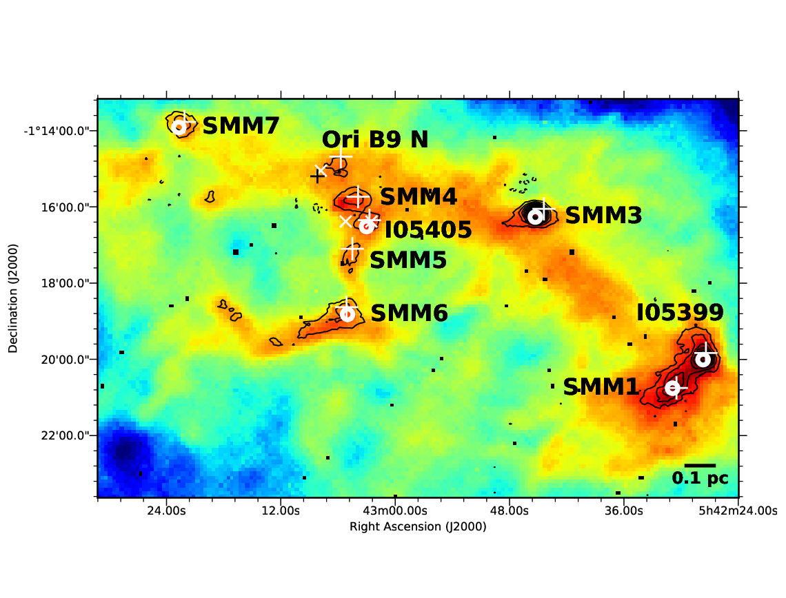
The target sample of the present study consists of the Orion B9 prestellar cores SMM 1, 6, and 7, and the protostellar cores IRAS 05399, IRAS 05405, and SMM 3. Besides spanning different early evolutionary stages, these six sources were selected for this study because their spatial distribution covers different parts of the Orion B9 region (see Fig. 1). The source list is given in Table 1.
The SABOCA 350 m peak positions of the aforementioned target sources were observed with the 12 m APEX telescope at the frequency of the o-H2D transition, that is GHz (Cologne Database for Molecular Spectroscopy (CDMS33 3 http://www.astro.uni-koeln.de/cdms; Müller et al. 2005)). The observations were carried out on 27-30 August and 15-16 December 2019, and the amount of precipitable water vapour (PWV) during the observations was measured to be between 0.3 mm and 1 mm, which corresponds to a zenith atmospheric transmission range of about 75--43% at the observed frequency44 4 The APEX atmospheric transmission calculator is available at http://www.apex-telescope.org/sites/chajnantor/atmosphere/transpwv/..
As a front end we used the Large APEX sub-Millimetre Array (LAsMA), which is a seven-pixel sideband separating (2SB) heterodyne array receiver that can be tuned within a frequency range of 273–374 GHz (Güsten et al. 2008). The backend was a Fast Fourier Transform fourth-Generation spectrometer (FFTS4G) that consists of two sidebands. Each sideband has two spectral windows of 4 GHz bandwidth, which provides both orthogonal polarisations and leads to a total bandwidth of 8 GHz. The o-H2D+ line was tuned in the upper sideband (USB). The 65 536 channels of the spectrometer yielded a spectral resolution of 61 kHz, which corresponds to 49 m s-1 at the observed frequency. The beam size (half-power beam width or HPBW) at the observed frequency is , which corresponds to a physical resolution of 0.034 pc.
The observations were performed in the wobbler-switching mode with a azimuthal throw between two positions on sky (symmetric offsets), and a chopping rate of Hz. The total on-source integration time (excluding overheads) was about 18–46 min depending on the source. The telescope focus and pointing were optimised and checked at regular intervals on the planet Uranus, the variable star o-Ceti, the asymptotic giant branch star R Doradus, and the carbon stars W Orionis and R Leporis. The pointing was found to be accurate to . The system temperatures during the observations were in the range K. Calibration was made by means of the chopper-wheel technique, and the output intensity scale given by the system is the antenna temperature corrected for the atmospheric attenuation (). The observed intensities were converted to the main-beam brightness temperature scale by , where is the main-beam efficiency. The value of at the observed frequency was calculated as follows. The aperture efficiency at the central frequency of LAsMA ( when estimated from observations towards Jupiter) was first scaled to that at the observed frequency using the Ruze formula (Ruze 1952), and then converted to the value of using the approximation formula . This yielded the values and .55 5 The APEX antenna efficiences can be found at http://www.apex-telescope.org/telescope/efficiency/index.php. The absolute calibration uncertainty was estimated to be about 10% (e.g. Dumke & Mac-Auliffe 2010).
The spectra were reduced using the Continuum and Line Analysis Single-dish Software (CLASS90) program of the GILDAS software package66 6 Grenoble Image and Line Data Analysis Software (GILDAS) is provided and actively developed by Institut de Radioastronomie Millimétrique (IRAM), and is available at http://www.iram.fr/IRAMFR/GILDAS. (version mar19b). The individual spectra were averaged with weights proportional to the integration time, divided by the square of the system temperature (). The resulting spectra were smoothed using the Hann window function to a velocity resolution of 98 m s-1 to improve the signal-to-noise ratio. Linear (first-order) baselines were determined from the velocity ranges free of spectral line features, and then subtracted from the spectra. The resulting rms noise levels at the 98 m s-1 velocity resolution were 28–33 mK on a scale. The observational parameters are provided in Table 2.
In Table 3, we summarise all the spectral line observations that were employed in the present study. In addition to the newly detected spectral lines, we also used spectral line data from Miettinen et al. (2010, 2012), Miettinen & Offner (2013b), and Miettinen (2016).
| Source | Type | |||
|---|---|---|---|---|
| [h:m:s] | [::] | [] | ||
| IRAS 05399-0121 | 05 42 27.7 | -01 20 00.4 | 11.3 | Class 0/I |
| SMM 1 | 05 42 30.9 | -01 20 45.4 | 6.0 | prestellar |
| SMM 3 | 05 42 45.3 | -01 16 16.0 | 18.7 | Class 0 |
| IRAS 05405-0117 | 05 43 03.0 | -01 16 31.0 | 11.0 | Class 0 |
| SMM 6 | 05 43 05.0 | -01 18 49.3 | 11.4 | prestellar |
| SMM 7 | 05 43 22.7 | -01 13 55.0 | 12.7 | prestellar |
| Source | PWV | a aa a aa The system temperature and rms noise level are given in the main-beam brightness temperature scale. | rms a aa a aa The system temperature and rms noise level are given in the main-beam brightness temperature scale. | |
|---|---|---|---|---|
| [min] | [mm] | [K] | [mK] | |
| IRAS 05399-0121 | 46.4 | 0.6-1.0 | 655 | 28 |
| SMM 1 | 32.1 | 0.6-1.0 | 600 | 33 |
| SMM 3 | 22.4 | 0.3-1.0 | 581 | 33 |
| IRAS 05405-0117 | 38.4 | 0.4-1.0 | 605 | 28 |
| SMM 6 | 17.6 | 0.4-1.0 | 459 | 29 |
| SMM 7 | 20.8 | 0.4-1.0 | 468 | 29 |
| Transition | HPBW | a aa a aa Offset with respect to the present o-H2D+ target positions. When this offset is different for different target source, a range of values is quoted (cf. Table 1). | Reference | |||
| [MHz] | [] | [pc] | [] | [pc] | ||
| o-H2D | 372 421.35580 | 16.8 | 0.034 | 0 | 0 | This work |
| N2H | 372 672.526 | 16.7 | 0.034 | 0 | 0 | This work |
| DCO | 360 169.7771 | 17.3 | 0.035 | 0 | 0 | This work |
| C18O | 219 560.3568 | 28.4 | 0.058 | 2.2 | 0.004 | Miettinen 2016 b bb b bb The C18O line was observed only towards SMM 3. |
| C17O | 224 714.199 | 27.8 | 0.057 | 0 | 0 | Miettinen & Offner 2013b c cc c cc Miettinen & Offner (2013b) studied the prestellar core SMM 6 (their source SMM 6a corresponds to the present target position). |
| … | … | … | 6.0-18.7 | 0.012-0.038 | Miettinen et al. 2012 | |
| N2D | 231 321.912 | 27.0 | 0.055 | 0 | 0 | Miettinen & Offner 2013b c cc c cc Miettinen & Offner (2013b) studied the prestellar core SMM 6 (their source SMM 6a corresponds to the present target position). |
| … | … | … | 6.0-18.7 | 0.012-0.038 | Miettinen et al. 2012 | |
| p-NH | 23 694.4955 | 40 | 0.081 | 6.0-18.7 | 0.012-0.038 | Miettinen et al. 2010 |
| p-NH | 23 722.6333 | 40 | 0.081 | 6.0-18.7 | 0.012-0.038 | Miettinen et al. 2010 |
3 Analysis and results
3.1 Spectral line analysis
The o-H2D spectra are shown in Fig. 2. The detected lines were fitted by single Gaussian functions using CLASS90. The obtained line parameters are listed in Table 4. In addition to the formal fitting errors output by CLASS90, the errors in the peak intensity () and the integrated intensity of the line () also include the 10% calibration uncertainty, which were added in quadrature.
The observed frequency bands revealed the presence of two additional spectral lines towards the target sources. The N2H line at 372 672.526 GHz in the USB was detected towards four target sources, while DCO at 360 169.7771 GHz in the lower sideband (LSB) was detected in all of our target sources (see the second and third row in Table 3). These additional line detections and their analysis are presented in more detail in Appendix A.


| Source | a aa a aa Peak optical thickness calculated using from the last column. | b bb b bb The value of was assumed to be equal to (Miettinen et al. 2010). | ||||
|---|---|---|---|---|---|---|
| [km s-1] | [km s-1] | [K] | [K km s-1] | [K] | ||
| IRAS 05399-0121 | … | … | c cc c cc A upper limit is placed for the non-detections. | d dd d dd The integrated intensity upper limit for these protostellar cores was estimated as the intensity upper limit ( K) times the detected linewidth in the Class 0 object SMM 3 (0.74 km s-1). | ||
| SMM 1 | ||||||
| SMM 3 | ||||||
| IRAS 05405-0117 | … | … | c cc c cc A upper limit is placed for the non-detections. | d dd d dd The integrated intensity upper limit for these protostellar cores was estimated as the intensity upper limit ( K) times the detected linewidth in the Class 0 object SMM 3 (0.74 km s-1). | ||
| SMM 6 | ||||||
| SMM 7 |
3.2 Molecular column densities and fractional abundances
The beam-averaged o-H2D+ column densities were calculated by using the standard, local thermodynamic equilibrium (LTE)-based formula,
| (2) |
where is the Planck constant, is the vacuum permittivity, is the permanent electric dipole moment, is the line strength, is the partition function, is the excitation temperature, is the -level degeneracy, is the reduced nuclear spin degeneracy, is the upper-state energy, is the Boltzmann constant, the function is defined as , and, for a Gaussian profile, the last integral term can be expressed as
| (3) |
where is the peak optical thickness of the line.
The value of the product for the observed o-H2D+ transition, D2, was taken from the Splatalogue database1111 11 http://www.cv.nrao.edu/php/splat/ (the CDMS value therein). We assumed that the o-H2D transition is thermalised at the NH3-based gas kinetic temperature derived by Miettinen et al. (2010) towards the target sources, that is ; see Table 4. This assumption is supported by the results of Caselli et al. (2008), where the ratio for their sample ranges from 1 to 1.47 (at a critical density of cm-3), with a mean (median) of 1.1 (1.0). The partition function values at the aforementioned values were interpolated from the values computed by Friesen et al. (2010; Table 3 therein). Because H2D+ is an asymmetric top molecule (the rotational constants from the CDMS database yield a Ray’s asymmetry parameter of (Ray 1932)), the value of is unity (i.e. no -level degeneracy), while for the observed ortho form of H2D+ (Turner 1991). The value of is 17.8 K (e.g. Friesen et al. 2010). The values of were calculated from the antenna equation (; see e.g. Eq. (1) in Miettinen et al. 2009) using the aforementioned NH3-based values and assuming that the background temperature is equal to that of the cosmic microwave background (CMB) radiation, that is K (Fixsen 2009).
The fractional abundances of o-H2D+ were calculated by dividing the o-H2D+ column density by the H2 column density, that is . The values were derived from our LABOCA dust continuum data re-reduced by Miettinen (2016). The angular resolution of the corresponding LABOCA image, (HPBW), is comparable to the beam size of our o-H2D+ observations (only a factor of 1.18 difference). We employed the standard formula that relates with the dust peak surface brightness (see e.g. Eq. (3) in Miettinen et al. 2009). We assumed that the dust temperature is equal to derived by Miettinen et al. (2010), the mean molecular weight per H2 molecule is 2.82, the dust opacity at 870 m is 1.38 cm2 g-1, and that the dust-to-gas mass ratio is (see Miettinen 2016 and references therein for the details).
In the present study, we also employ the C17O, N2H+, and N2D+ data from Miettinen et al. (2012) and Miettinen & Offner (2013b), and C18O data from Miettinen (2016; only for SMM 3). The column densities of these linear molecules were also re-calculated using Eq. (2) so that they can be compared with the present o-H2D+ results (e.g. Miettinen et al. (2012) employed a non-LTE approach in their column density analysis). The C17O and C18O lines were assumed to be thermalised at , while the values were used for N2H+ and N2D+ (we refer to Miettinen 2016 for a more detailed description). To properly calculate the fractional abundances of the aforementioned linear molecules, the corresponding values were derived from the LABOCA data smoothed to the coarser resolution of the line observations ( HPBW). The beam-averaged column densities and abundances with respect to H2 calculated in this section are given in Table 5. The column densities and fractional abundances calculated from the additional spectral line detections are presented in Appendix A.
| Source | ||||||||
|---|---|---|---|---|---|---|---|---|
| [ cm-2] | [] | [ cm-2] | [] | [ cm-2] | [] | [ cm-2] | [] | |
| IRAS 05399-0121 | ||||||||
| SMM 1 | ||||||||
| SMM 3 | a aa a aa The column density and fractional abundance of the C18O isotopologue derived from observations towards the Spitzer 24 m peak position ( offset from the SABOCA peak) are cm-2 and , respectively (Miettinen 2016). | a aa a aa The column density and fractional abundance of the C18O isotopologue derived from observations towards the Spitzer 24 m peak position ( offset from the SABOCA peak) are cm-2 and , respectively (Miettinen 2016). | ||||||
| IRAS 05405-0117 | ||||||||
| SMM 6 b bb b bb The values on the first row for SMM 6 refer to the SABOCA 350 m peak position (Miettinen & Offner 2013b; their source SMM 6a), while those on the second row were derived towards our earlier target position (Miettinen et al. 2012). | ||||||||
| … | … | |||||||
| SMM 7 | c cc c cc The N2D line was not detected towards SMM 7 (Miettinen et al. 2012), and hence we estimated the column density upper limit from the line intensity upper limit and the N2H linewidth divided by the average ratio () in our sample. All the quoted upper limits take the uncertainties into account. |
3.3 CO depletion factor and the degree of deuterium fractionation
To estimate the factors by which the CO molecules are depleted in the target cores, we followed the analysis presented in Miettinen et al. (2012) with the modifications employed by Miettinen (2016). In short, the canonical or undepleted CO abundance was assumed to be , and the and oxygen isotope ratios needed in the analysis were assumed to be 557 and 4.16, respectively (see Miettinen 2016 and references therein). The CO depletion factor was then calculated as , where the denominator is the observed CO abundance.
The degree of deuterium fractionation in N2H+ was calculated by dividing the column density of N2D+ by that of N2H+. The values of and are tabulated in Table 6.
3.4 CO depletion timescale
The rate at which CO molecules freeze out onto dust grain surfaces, , can be used to calculate the CO depletion timescale as (e.g. Rawlings et al. 1992; Maret et al. 2013)
| (4) |
where is the grain number density, is the mean geometric grain cross section with being the average grain radius (assumed to be 0.1 m), is the mean thermal speed of the CO molecules, and is their sticking coefficient. The grain number density can be expressed as , where is the fractional abundance of dust grains and is the H2 number density. The value of can be solved from the equality , where is the mass of a dust grain and is that of the H2 molecule. Under the assumption of spherical dust grains, the mass of a grain is given by , where is the mass density of a grain (assumed to be 3 g cm-3). For a Maxwellian distribution of gas-phase CO molecules, the mean thermal speed is given by , where is the mass of the CO molecule. Finally, we assumed that , which signifies that the CO molecules stick to the dust grains in each collision, which is expected to be a reasonable assumption at the low temperatures of the present target sources (Burke & Hollenbach 1983; Bisschop et al. 2006).
The volume-averaged H2 number densities and the corresponding CO depletion timescales of the target sources are listed in Table 6. The former values were adopted from our previous studies of the Orion B9 cores (Miettinen et al. 2010, 2012; Miettinen & Offner 2013b), but they were scaled upward owing to the present assumptions about the source distance and dust properties.
3.5 Correlation plots
To search for potential correlations between the different parameters derived in the present paper and our earlier studies, we made several scatter plots that are useful to visualise the relationship between two variables. Figure. 3 shows the degree of deuterium fractionation, or the ratio, as a function of the o-H2D+ abundance, CO depletion factor, and the gas kinetic temperature derived from NH3 by Miettinen et al. (2010). The o-H2D+ abundance is also shown as a function of the CO depletion timescale and the CO depletion factor as a function of the NH3-based gas temperature. The prestellar and protostellar cores are shown in different colours (blue and red, respectively) to better illustrate how the corresponding data points populate the plotted parameter spaces.
Figure 4 shows the o-H2D+ abundance as a function of the gas kinetic temperature. For comparison, the relationship between and derived by Caselli et al. (2008; their Eq. (7)) is indicated in Fig. 4.
We remind the reader that the C17O, NH3, N2H+, and N2D+ observations used to construct the plots in Figs. 3 and 4 were targeting the same positions. However, the new o-H2D+ observations were made towards positions offset from our previous molecular line observations (the mean offset is or 0.7 times the beam of the o-H2D+ observations; Table 1), except for SMM 6 for which we also have C17O, N2H+, and N2D+ data for the present target position (only offset; Miettinen & Offner 2013b).


4 Discussion
4.1 Interrelations between o-H2D+, CO depletion, and deuterium fractionation
Owing to the low deuteron affinity of the H2D+ molecule, it reacts eagerly with other species by donating a deuteron (e.g. Roberts et al. 2002). Therefore, deuterium enrichements are passed forward to heavier species. For example, one-third of the reactions between H2D+ and molecular nitrogen yield N2D+ (the remaining two-thirds lead to N2H+). The deuterium fractionation in a given species, such as N2H+ for example, is therefore expected to become higher for a higher abundance of H2D+. Despite the angular offset between the N2H+, N2D+, and o-H2D+ observations (Sect. 3.5), this is qualitatively consistent with what we see in the top left panel in Fig. 3, that is the highest ratios are seen at the highest o-H2D+ abundances (and vice versa).
The H2D+ molecules are mainly destroyed in reactions with CO, which yield either HCO+ or DCO+. Therefore, the less gas-phase CO there is, the lower the destruction rate of H2D+ (e.g. Roberts & Millar 2000). In other words, the higher the CO depletion factor, the higher the expected deuteration degree (e.g. Vastel et al. 2006). Although the data points plotted in the top middle panel in Fig. 3 show a large scatter, the prestellar and protostellar core populations are each qualitatively consistent with the aforementioned description, that is the highest ratios are associated with the highest levels of CO depletion (see Sect. 4.2).
Because the level of CO depletion via freeze-out becomes higher at higher gas densities (e.g. Bacmann et al. 2002), one would also expect higher values, and hence higher deuteration levels at lower gas temperatures (e.g. Emprechtinger et al. 2009). These trends are not visible in the top right and bottom right panels of Fig. 3. If anything, there appears to be a positive correlation between and among the prestellar cores. However, the gas temperature range explored here is fairly narrow, from K to K, which might render the trend imperceptible. Another potential issue is the fact that the gas temperatures plotted in Fig. 3 were derived from the and inversion lines of para-NH3, which have a much lower critical density ( cm-3) than the transitions of N2H+ and N2D+ ( cm-3) from which the deuteration level was derived (Miettinen et al. 2010, 2012; Miettinen 2016). Therefore, the derived ratios and values might refer to different gas components, which would explain the lack of the expected negative correlation in the top right panel of Fig. 3.
| Source | ||||
|---|---|---|---|---|
| [ cm-3] | [ yr] | |||
| IRAS 05399-0121 | ||||
| SMM 1 | ||||
| SMM 3 a aa a aa The CO depletion factor quoted on the first row was derived from the C18O observations towards the Spitzer 24 m peak position of the source, which lies to the north-west of the SABOCA peak (Miettinen 2016), while the values on the second row were derived towards our earlier target position (Miettinen et al. 2012). | … | … | … | |
| IRAS 05405-0117 | ||||
| SMM 6 b bb b bb The values on the first row for SMM 6 refer to the SABOCA 350 m peak position (Miettinen & Offner 2013b; their source SMM 6a), while those on the second row were derived towards our earlier target position (Miettinen et al. 2012). | ||||
| SMM 7 |
4.2 Comparison of the H2D+-based deuteration between the prestellar and protostellar cores in Orion B9
As illustrated in the top left panel of Fig. 3, the studied prestellar cores show higher o-H2D+ abundances and deuteration ratios than the protostellar cores. This can be understood by considering the feedback effects from the protostar(s) deeply embedded in the protostellar cores. The central protostar increases its mass by accreting gas from the surrounding envelope via a circumstellar disk, and this process is associated with both heating of the surrounding medium and protostellar jets that drive molecular outflows. When the gas temperature exceeds K, reaction (1) starts to operate from right to left, which leads to the decrease of deuteration (e.g. Vastel et al. 2006). At the same time, thanks to both central heating and outflow shocks, CO molecules can be released from the icy grain mantles back into the gas phase, which leads to the destruction of H2D+.
That the prestellar cores populate a higher regime than the more evolved protostellar cores is also visible in the top middle and right panels in Fig. 3. Interestingly, the lowest CO depletion factor in our sample was derived for the prestellar core SMM 1, namely , which is consistent with no depletion. On the other hand, the protostellar core SMM 3 exhibits the highest level of CO depletion, , towards the core centre and towards the envelope ( or 0.034 pc projected separation). The Class 0 object SMM 3 is the strongest source of 350 m and 870 m emission in Orion B9 (Miettinen et al. 2009, 2012), and is therefore likely to be in a very early stage of protostellar evolution, where the dusty envelope is still resembling the properties that prevailed at its prestellar phase. The prestellar core SMM 1 on the other hand might be affected by the northwest-southeast oriented outflow driven by the nearby Class 0/I protostar IRAS 05399 (see Miettinen & Offner 2013a and references therein). This could increase the CO abundance in the gas phase in SMM 1 via outflow shock desorption, or simply by pushing extra CO gas towards SMM 1 that is being captured in our observations. We note that the outflow motions from IRAS 05399 are also indicated by the red asymmetric profile of the DCO line detected in the present work (see Fig. 8). Nevertheless, the low CO depletion factor in SMM 1 is still puzzling in terms of the high deuteration observed in the source (). Perhaps SMM 1 is seen in a specific stage, where the abundant CO molecules have not yet had time to bring down the deuteration in N2H+.
4.3 Orion B9 in a wider context of H2D+ studies of star-forming regions
As the main comparison sample of o-H2D+ observations towards dense cores, we used the Caltech Submillimeter Observatory (CSO) survey by Caselli et al. (2008). To our knowledge, the Caselli et al. (2008) study is the largest H2D+ survey published so far, and therefore provides a useful comparison sample with the present results. These authors observed the same o-H2D transition as we did towards ten starless cores and six protostellar cores. The line was detected in seven () and four () of these targets, respectively. We detected o-H2D+ in all three of our prestellar cores, but in only one of the three protostellar cores ( detection rate). We note that the Caselli et al. (2008) sample included a target position in Orion B9, which was called Ori B9, but that position is not coincident with any significant LABOCA dust emission (see Fig. 1), which probably explains their non-detection. As discussed in Sect. 1, the latter position is close to one of the positions observed in o-H2D+ by Harju et al. (2006; offset from their source Ori B9 N). We also note that Ori B9 is often considered to be a massive dense core in the literature (e.g. Harju et al. 2006; Caselli et al. 2008; Pillai et al. 2012), but the source is composed of a system of low-mass dense cores.
Caselli et al. (2008) used a somewhat different method to calculate the o-H2D+ column densities (e.g. their calculation made use of the photon escape probability), and therefore it is important to decipher whether or not the two methods lead to similar results. For this purpose, we took the line parameters for the two strongest o-H2D+ detections by Caselli et al. (2008), namely those towards L 1544 and L 183 (their Tables 2 and 3; the values valid at a critical density of cm-3), and derived values that agree within factors of (our nominal values being higher). We therefore conclude that the two methods yield results that are in good agreement with each other, and a direct comparison is reasonable.
The o-H2D+ line widths derived by Caselli et al. (2008) for their starless and protostellar cores are km s-1 and km s-1 (the authors adopted a line width of 0.42 km s-1 for Ori B9 from Harju et al. (2006), but that value refers to the starless source Ori B9 N, and is hence neglected from the latter range). The corresponding averages are 0.47 km s-1 and 0.93 km s-1. We found a factor 1.34 broader average o-H2D+ line width (0.63 km s-1) for our prestellar cores, which could indicate that Orion B9 is dynamic in nature (see Sect. 1). On the other hand, the line width for our only protostellar source detection (SMM 3; 0.74 km s-1) is comparable with those in the prestellar objects (only 1.17 times broader than the average line width for prestellar cores), which is at odds with the average trend in the Caselli et al. (2008) sample, but supports the aforementioned hypothesis that SMM 3 is in its very early Class 0 stage.
The o-H2D+ column densities derived for starless cores by Caselli et al. (2008) are cm-2, while those for protostellar cores are cm-2. The corresponding fractional abundances are and . The values for the Orion B9 prestellar cores are derived to be cm-2, with the corresponding fractional abundances being . Although the former values resemble the lower end values found by Caselli et al. (2008), our values are closer to the highest values in the CSO survey. Although the o-H2D+ column density we derived for SMM 3 is bracketed by the range derived by Caselli et al. (2008) for their dense cores associated with ongoing star formation, the value of the source () appears to be higher. However, derivation of the fractional abundances is susceptible to the assumptions used to calculate the H2 column density, and therefore it might be more reliable to compare the values.
The only significant correlation between core properties found by Caselli et al. (2008) was that between and (see our Fig. 4). Within the uncertainties, our results appear to be consistent with this relationship with a notable exception being the prestellar core SMM 6. However, a notable caveat in our analysis is that our values were derived from ammonia observations towards positions that are different from the present target positions (i.e. offsets from the SABOCA 350 m peak positions; Table 1), although the large beam size of the former data ( HPBW) encompasses the o-H2D+ targets. Nevertheless, despite this weakness in our methodology, at least half of our sources are consistent even with the nominal correlation derived by Caselli et al. (2008). As discussed above, the values of are sensitive to the way the corresponding are calculated, and this can also affect the comparison made here.
Regarding the validity of using the NH3-based gas temperature to compare with the o-H2D+ data, we also estimated the value of for SMM 6 from the observed line widths of o-H2D+ and N2D; see Miettinen & Offner 2013b. If the observed transitions of these two species originate in a common gas component, they should be sensitive to the same gas motions and gas temperature, which in turn would imply equally large non-thermal velocity dispersions (see Friesen et al. 2010; Eq. (7) therein). From the equality we derived a value of K for SMM 6, which agrees within the uncertainties with the value K derived by Miettinen et al. (2010). For comparison, using the N2H line width in the analysis (see Appendix A), the temperature estimate becomes higher, namely K. The former comparison is expected to be more accurate because N2D+ is formed from H2D+ (cf. Friesen et al. 2010), and supports the use of values in our analysis.
Caselli et al. (2008) suggested the following reasons for the negative relationship visible in their sample. First, the warmer the source, the smaller the o-H2D+-emitting region might be, which would lead to a beam dilution effect (the line intensity is diluted by the ratio of the solid angle subtended by the emission region to the beam solid angle). Secondly, the warmest sources in the Caselli et al. (2008) sample were generally identified as being the most distant ones ( pc), which could also be an issue owing to beam dilution. Thirdly, the physical and chemical interpretation is that the warmer the gas, the lower the degree of CO depletion, and hence the higher the destruction rate of H2D+. The authors also pointed out that the heating by a central protostar might not significantly increase the gas-phase CO abundance (as supported by the bottom right panel in our Fig. 3), but that the process might instead affect the ortho-para ratio of H2D+ in such a way that the o-H2D+ abundance decreases (see e.g. Sipilä et al. 2017 for the ortho-para conversion reactions of H2D+).
Pillai et al. (2012) derived values of cm-2 and values of towards five sources in the DR 21 filament of Cygnus X, which is a high-mass star-forming region. The authors assumed a value of 10 K for the whole sample and different dust properties from those assumed here to calculate the H2 column density (and hence ). Taking into account the differences in the dust opacity (, where the dust emissivity index is for our adopted dust model (see Miettinen & Offner 2013a and references therein)) and gas-to-dust mass ratio (we used a factor of 1.41 higher value), the fractional abundances reported by Pillai et al. (2012) should be scaled down by a factor of 0.47 for a more meaningful comparison. Our o-H2D+ column densities in the detected sources appear to be somewhat higher than in DR 21, but the upper limits for the protostellar cores IRAS 05399 and IRAS 05405 are less than the lowest value found by Pillai et al. (2012). Also, the o-H2D+ abundances we derived appear to be higher than in DR 21 (e.g. a factor of 30 difference between the highest values).
Giannetti et al. (2019) reported values of cm-2 towards three clumps in the G351.77-0.51 filament that have the potential to form high-mass stars. These column densities also appear to be lower than in our sample. Hence, the o-H2D+ abundances appear to be higher in low-mass star-forming regions than in massive star-forming regions. The process of low-mass star formation is characterised by at least an order of magnitude longer (and colder) starless core phase compared to that of high-mass stars (e.g. Brünken et al. 2014; Tigé et al. 2017), which supports the development of matured deuterium chemistry in low-mass dense cores.
4.4 Relative abundances of o-H2D+, N2D+, and DCO+ as evolutionary indicators
Giannetti et al. (2019) found that as the clump evolves, the o-H2D+ abundance drops while that of N2D+ behaves in the opposite way, and hence the [o- ratio decreases as a function of evolution (see their Fig. 3). The authors suggested that this trend could be caused by the conversion of H2D+ to the doubly and triply deuterated species D2H+ and D ( and ), associated with the formation of N2D+ in the reactions and (e.g. Pagani et al. 2009a, 2011). In the protostellar stage, where the gas-phase CO abundance is expected to be higher than in the starless phase (at least near the central protostar), the H2D+ and N2D+ molecules are being destroyed by CO. Also, the reverse reaction (1) becomes relevant at higher temperatures, which leads to the drop of the [o- ratio. To examine if the sources in our sample exhibit such a trend, we first estimated the relative evolutionary stages of the target prestellar cores using the CO depletion timescales derived in Sect. 3.4. The chemical CO depletion timescale can be interpreted as a lower limit to the age of the core (Maret et al. 2013), and the values given in Table 6 suggest that SMM 6 could be the youngest prestellar core in our sample (age yr), followed by SMM 1 ( yr) and SMM 7 ( yr). We note that in the present study we observed the densest condensation in SMM 6 (Miettinen & Offner 2013b; their source SMM 6a), while the CO depletion timescale derived for the lower density elongated parent core suggests an age of yr.
Miettinen et al. (2009, 2012) studied the spectral energy distributions (SEDs) of the Orion B9 protostellar cores (see also Miettinen & Offner 2013a; Miettinen 2016). As part of the SED analysis, the authors derived the ratios of the sources, where is the total (gas plus dust) mass of the core (essentially the envelope mass) and is the bolometric luminosity. This ratio is found to decrease with time (it is related to the weakening of the protostellar outflow strength), and can therefore be used as an evolutionary indicator (Bontemps et al. 1996). On the basis of this analysis, SMM 3 is the youngest protostellar core in our sample, followed by IRAS 05405 and then IRAS 05399. Indeed, in our earlier studies we found that SMM 3 and IRAS 05405 are Class 0 objects, while IRAS 05399 appears to be in the transition phase from Class 0 to I.
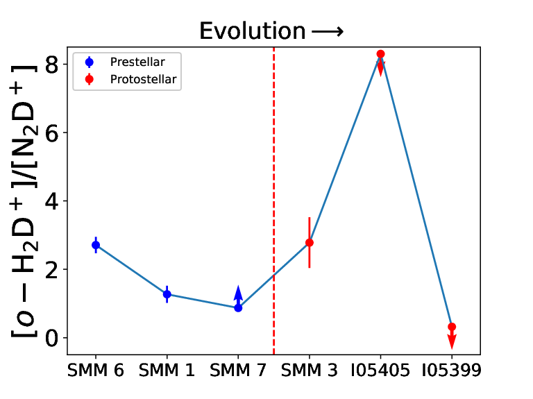
Under the assumption of the aforementioned evolutionary sequence, in Fig. 5 we plot the fractional abundances of o-H2D+ and N2D+ and the [o- ratio (calculated from the column densities) as a function of source evolution. Indeed, the o-H2D+ abundance appears to drop as the core evolves in agreement with the finding by Giannetti et al. (2019). We note that the o-H2D+ abundances in SMM 1 and SMM 7 are very similar to each other (their ratio is ), but so are their CO depletion times (with a ratio of ), which suggests that the cores are in comparable stages of evolution (cf. the bottom left panel in Fig. 3). However, the behaviour of the N2D+ abundance is more fluctuating, which might be a manifestation of the fact that our N2D+ observations were offset from the core centres (except for SMM 6).
As a result of the aforementioned fluctuation in the observed N2D+ abundance, the relative abundance of o-H2D+ and N2D+ does not exhibit a clear decreasing trend with core evolution as found by Giannetti et al. (2019). However, owing to the censored values (especially the upper [o-]/ limits for IRAS 05405 and IRAS 05399), the existence of a decreasing trend is still possible, although SMM 3 would still be an outlier from such trend.
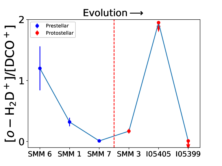
Figure 6 is similar to Fig. 5 but DCO+ was used in the analysis instead of N2D+ (see Appendix A). The DCO data were observed from the exact same positions as the o-H2D+ data (and simultaneosly in the observed frequency bands). Another benefit of using DCO+ in the analysis is that the species was detected towards all six target sources. The DCO+ abundance does not appear to exhibit any evolutionary trend, and the [o- ratio behaves in a similar way as the [o- ratio. However, the prestellar regime shows a somewhat stronger hint of a decreasing trend than in the case of [o-. If the decrease of the o-H2D+ abundance is indeed driven by its conversion to D2H+ and D, then DCO+ can form in the reactions and (e.g. Pagani et al. 2009a, 2011). On the other hand, the DCO+ formation via these reactions is confronted by the abundance of gas-phase CO, which is first expected to decrease as the core evolves in its prestellar stage, and then to increase in the protostellar stage owing to desorption of icy grain mantles. The difference compared to the case of N2D+ above is that even if the gas-phase CO abundance is very low owing to its depletion, the gas can still be rich in N2. For example, N2 has about 18% lower binding energy than CO, and therefore N2 can evaporate from dust grain mantles more quickly (see Giannetti et al. 2019 and references therein). Another chemical pathway that can contribute to the formation of DCO+ is the reaction , followed by the reaction (e.g. Favre et al. 2015; Salinas et al. 2017). However, because the latter reactions are relevant at warm temperatures of K, they are expected to play a role in the formation of DCO+ around the hot corinos of low-mass protostellar cores, where the temperature is K (see Ceccarelli et al. 2007 for a review).
To summarise, although we found that the o-H2D+ abundance drops as the core evolves, the reliability of using of the [o- and [o- abundance ratios as evolutionary indicators remains inconclusive. Larger source samples and observations of additional deuterated species like D2H+ would be particularly useful to better understand the temporal behaviour of the abundances of H2D+, N2D+, and DCO+.


4.5 Chance superposition cores and other line-of-sight gas components seen towards Orion B9
While the LSR velocities of the detected o-H2D+ lines are about 9 km s-1, the o-H2D+ emission from the prestellar core SMM 7 appears at km s-1. This is also the case for the detected DCO lines (see Appendix A). Indeed, Miettinen et al. (2010, 2012) found that the NH, NH, C17O, DCO, and N2H line emissions towards SMM 7 occur at 3.6-4 km s-1. These results suggest that SMM 7 might be a chance projection seen towards the Orion B9 filament.
Moreover, the protostellar source IRAS 05413-0104 that lies (1.6 pc) to the northeast of SMM 7 (see Fig. 1 in Miettinen et al. 2009) was found to have NH3 radial velocities that are significantly lower than the bulk of the Orion B9 cores, namely km s-1 (Miettinen et al. 2010). Also, the protostellar core SMM 4, which was not chosen for the present study, was found to exhibit line emission at 1.5-1.7 km s-1 by Miettinen et al. (2012), although the NH3 lines detected towards SMM 4 showed two components, one at the systemic velocity of Orion B9 ( km s-1) and the other at about 1.6 km s-1. This could be caused by the large, beam of the NH3 observations that also captured the 9 km s-1 gas component (see Fig. 1). Therefore, in addition to SMM 7, the protostellar cores SMM 4 and IRAS 05413 may also be physically unrelated to the Orion B9 star-forming region.
One of the present target sources, IRAS 05405, exhibits additional velocity components in the C17O and N2D spectra (Miettinen et al. 2012). As was pointed out by Miettinen et al. (2010), the dense gas and dust associated with the additional line-of-sight velocity components can also affect the physical parameters of the cores derived from dust continuum observations. For example, the dust-based H2 column density can be overestimated if the dust continuum surface brightness is contaminated by a physically unrelated component. This would then lead to underestimated fractional abundances of the detected molecules. For instance, the lower velocity C17O lines detected towards IRAS 05405 (at 1.3 km s-1 and 3.0 km s-1) are of the intensity of the systemic velocity (9.2 km s-1) line (Miettinen et al. 2012; Table 5 therein). However, the beam size of the aforementioned C17O observations was 1.65 times larger than that of the present o-H2D+ observations, and therefore the contribution from the additional line-of-sight velocity components to the present o-H2D+ abundance upper limit is unclear. Moreover, the H2 column density estimates suffer from other uncertain parameters, especially from the uncertainty in the submillimetre dust opacity that can be a factor of approximately two (e.g. Shirley et al. 2011). In conclusion, the additional velocity components seen towards Orion B9 are relevant for only one of the present targets (IRAS 05405), but their relative contribution to the submillimetre dust continuum emission is difficult to reliably quantify. High-resolution molecular line imaging would be useful to resolve this issue.
5 Summary and conclusions
We used the APEX telescope to observe the 372 GHz o-H2D line towards three prestellar cores and three protostellar cores in the Orion B9 filament. The o-H2D+ data were analysed in conjunction with our previous APEX spectral line and dust continuum data for the target sources. Our main results are summarised as follows:
- 1.
The o-H2D line was detected in all three prestellar cores with the abundances in the range . Only one of the protostellar cores, the Class 0 object SMM 3, was detected in o-H2D+ emission with an abundance of .
- 2.
Besides the o-H2D+ line detections, the N2H line was detected towards all the sources except one prestellar core (SMM 7), and DCO was detected in all the target sources.
- 3.
No significant correlations were found between the level of deuterium fractionation (quantified as the ratio), the factor of CO depletion, the gas kinetic temperature derived from ammonia, or the o-H2D+ abundance. However, our results are in fairly good agreement with the relationship derived by Caselli et al. (2008) for low-mass dense cores.
- 4.
The derived o-H2D+ abundances in Orion B9 are more similar to those observed in other low-mass star-forming regions than to those derived for high-mass star-forming clumps where the values are typically a few times or less.
- 5.
We found that the o-H2D+ abundance appears to decrease as a function of temporal core evolution. We also addressed the evolutionary scenario proposed by Giannetti et al. (2019), namely that the [o- abundance ratio decreases as the core evolves towards more advanced stages. However, our results were not conclusive, which might (partly) be caused by the spatial offset between our o-H2D+ and N2D+ observations ( on average). Indeed, the N2D+ abundance was not found to increase as the core evolves, but it rather showed a fluctuating behaviour. On the other hand, the [o- ratio, where the DCO+ data were observed simultaneously with o-H2D+, was also not found to exhibit any clear evolutionary trend.
- 6.
The prestellar core SMM 7 exhibits o-H2D+ line emission at a radial velocity that is almost km s-1 lower than the systemic velocity of Orion B9. Therefore, the source might be a chance projection seen towards the Orion B9 filament region.
Orion B9 is part of the dynamic Orion B environment, and could itself be a region of triggered core and star formation that lies about pc from the H II region NGC 2024. However, large-scale molecular line mapping (covering at least the whole Orion B9 filament) is required to better understand the line-of-sight velocity distribution of Orion B9, and to quantitatively test the hypothesis that the region is indeed affected by feedback processes. If confirmed, the Orion B9 filament provides an interesting target system to investigate the deuterium-based chemistry and the possible environmental effects in an important class of star-forming regions. Observations of the para form of H2D+ would be useful to constrain the ages of the cores (Brünken et al. 2014; Harju et al. 2017), and thus the age of the whole parent filament. Also, to better understand the behaviour of the [o- evolutionary indicator proposed by Giannetti et al. (2019), observations of D2H+ would be useful to investigate the importance of the deuteration sequence in dense cores destined to become new stars.
Acknowledgements.
I thank the referee for the critical comments and suggestions. I am grateful to the staff at the APEX telescope for performing the service mode LAsMA observations presented in this paper. I would also like to thank Sébastien Bardeau and Sébastien Maret for the help with the GILDAS software package. This research has made use of NASA’s Astrophysics Data System Bibliographic Services. This research made use of Astropy1414 14 http://www.astropy.org, a community-developed core Python package for Astronomy (Astropy Collaboration et al. 2013, 2018 2018).References
- André et al. (2010) André, P., Men’shchikov, A., Bontemps, S., et al. 2010, A&A, 518, L102
- Angerhofer et al. (1978) Angerhofer, P., Churchwell, E., & Porter, R. N. 1978, Astrophys. Lett., 19, 137
- Astropy Collaboration et al. (2013) Astropy Collaboration, Robitaille, T. P., Tollerud, E. J., et al. 2013, A&A, 558, A33
- (4) Astropy Collaboration, Price-Whelan, A. M., Sipőcz, B. M., et al. 2018, AJ, 156, 123
- Bacmann et al. (2002) Bacmann, A., Lefloch, B., Ceccarelli, C., et al. 2002, A&A, 389, L6
- Bally (2008) Bally, J. 2008, in Handbook of Star Forming Regions, ed. B. Reipurth, Volume I, p. 459
- Bergin & Tafalla (2007) Bergin, E. A., & Tafalla, M. 2007, ARA&A, 45, 339
- Bisschop et al. (2006) Bisschop, S. E., Fraser, H. J., Öberg, K. I., et al. 2006, A&A, 449, 1297
- Bontemps et al. (1996) Bontemps, S., André, P., Terebey, S., et al. 1996, A&A, 311, 858
- Brünken et al. (2014) Brünken, S., Sipilä, O., Chambers, E. T., et al. 2014, Nature, 516, 219
- Burke & Hollenbach (1983) Burke, J. R., & Hollenbach, D. J. 1983, ApJ, 265, 223
- Caselli & Myers (1994) Caselli, P., & Myers, P. C. 1994, in Clouds, Cores, and Low Mass Stars, ASPC, Vol. 65, p. 52
- Caselli et al. (2008) Caselli, P., Vastel, C., Ceccarelli, C., et al. 2008, A&A, 492, 703
- Ceccarelli et al. (2007) Ceccarelli, C., Caselli, P., Herbst, E., et al. 2007, in Protostars and Planets V, ed. B. Reipurth, D. Jewitt, and K. Keil (Tucson: Univ. of Arizona Press), p. 47
- Cowie et al. (1979) Cowie, L. L., Songaila, A., & York, D. G. 1979, ApJ, 230, 469
- Dalgarno & Lepp (1984) Dalgarno, A., & Lepp, S. 1984, ApJ, 287, L47
- Dumke & Mac-Auliffe (2010) Dumke, M., & Mac-Auliffe, F. 2010, Proc. SPIE, 77371J
- Emprechtinger et al. (2009) Emprechtinger, M., Caselli, P., Volgenau, N. H., et al. 2009, A&A, 493, 89
- Favre et al. (2015) Favre, C., Bergin, E. A., Cleeves, L. I., et al. 2015, ApJ, 802, L23
- Fixsen (2009) Fixsen, D. J. 2009, ApJ, 707, 916
- Friesen et al. (2010) Friesen, R. K., Di Francesco, J., Myers, P. C., et al. 2010, ApJ, 718, 666
- Friesen et al. (2014) Friesen, R. K., Di Francesco, J., Bourke, T. L., et al. 2014, ApJ, 797, 27
- Gerlich et al. (2002) Gerlich, D., Herbst, E., & Roueff, E. 2002, Planet. Space Sci., 50, 1275
- Giannetti et al. (2019) Giannetti, A., Bovino, S., Caselli, P., et al. 2019, A&A, 621, L7
- Güsten et al. (2006) Güsten, R., Nyman, L. Å., Schilke, P., et al. 2006, A&A, 454, L13
- Güsten et al. (2008) Güsten, R., Baryshev, A., Bell, A., et al. 2008, Proc. SPIE, 702010
- Harju et al. (2006) Harju, J., Haikala, L. K., Lehtinen, K., et al. 2006, A&A, 454, L55
- Harju et al. (2008) Harju, J., Juvela, M., Schlemmer, S., et al. 2008, A&A, 482, 535
- Harju et al. (2017) Harju, J., Sipilä, O., Brünken, S., et al. 2017, ApJ, 840, 63
- Kounkel et al. (2017) Kounkel, M., Hartmann, L., Loinard, L., et al. 2017, ApJ, 834, 142
- Maret et al. (2011) Maret, S., Hily-Blant, P., Pety, J., et al. 2011, A&A, 526, A47
- Maret et al. (2013) Maret, S., Bergin, E. A., & Tafalla, M. 2013, A&A, 559, A53
- Miettinen (2012) Miettinen, O. 2012, A&A, 545, A3
- Miettinen (2016) Miettinen, O. 2016, Ap&SS, 361, 248
- (35) Miettinen, O., & Offner, S. S. R. 2013a, A&A, 553, A88
- (36) Miettinen, O., & Offner, S. S. R. 2013b, A&A, 555, A41
- Miettinen et al. (2009) Miettinen, O., Harju, J., Haikala, L. K., et al. 2009, A&A, 500, 845
- Miettinen et al. (2010) Miettinen, O., Harju, J., Haikala, L. K., et al. 2010, A&A, 524, A91
- Miettinen et al. (2012) Miettinen, O., Harju, J., Haikala, L. K., et al. 2012, A&A, 538, A137
- Müller et al. (2005) Müller, H. S. P., Schlöder, F., Stutzki, J., et al. 2005, Journal of Molecular Structure, 742, 215
- Neugebauer et al. (1984) Neugebauer, G., Habing, H. J., van Duinen, R., et al. 1984, ApJ, 278, L1
- Ohama et al. (2017) Ohama, A., Tsutsumi, D., Sano, H., et al. 2017, PASJ, submitted, arXiv:1706.05652
- Pagani et al. (1992) Pagani, L., Wannier, P. G., Frerking, M. A., et al. 1992, A&A, 258, 472
- (44) Pagani, L., Vastel, C., Hugo, E., et al. 2009a, A&A, 494, 623
- (45) Pagani, L., Daniel, F., & Dubernet, M.-L. 2009b, A&A, 494, 719
- Pagani et al. (2011) Pagani, L., Roueff, E., & Lesaffre, P. 2011, ApJ, 739, L35
- Phillips et al. (1985) Phillips, T. G., Blake, G. A., Keene, J., et al. 1985, ApJ, 294, L45
- Pickett et al. (1998) Pickett, H. M., Poynter, R. L., Cohen, E. A., et al. 1998, J. Quant. Spec. Radiat. Transf., 60, 883
- Pillai et al. (2012) Pillai, T., Caselli, P., Kauffmann, J., et al. 2012, ApJ, 751, 135
- Pilbratt et al. (2010) Pilbratt, G. L., Riedinger, J. R., Passvogel, T., et al. 2010, A&A, 518, L1
- Rawlings et al. (1992) Rawlings, J. M. C., Hartquist, T. W., Menten, K. M., et al. 1992, MNRAS, 255, 471
- Ray (1932) Ray, B. S. 1932, Z. Physik, 78, 74
- Roberts & Millar (2000) Roberts, H., & Millar, T. J. 2000, A&A, 361, 388
- Roberts et al. (2002) Roberts, H., Herbst, E., & Millar, T. J. 2002, MNRAS, 336, 283
- Ruze (1952) Ruze, J. 1952, Il Nuovo Cimento, 9, 364
- Salinas et al. (2017) Salinas, V. N., Hogerheijde, M. R., Mathews, G. S., et al. 2017, A&A, 606, A125
- Schneider et al. (2013) Schneider, N., André, P., Könyves, V., et al. 2013, ApJ, 766, L17
- Shirley et al. (2011) Shirley, Y. L., Huard, T. L., Pontoppidan, K. M., et al. 2011, ApJ, 728, 143
- Sipilä et al. (2017) Sipilä, O., Harju, J., & Caselli, P. 2017, A&A, 607, A26
- Siringo et al. (2009) Siringo, G., Kreysa, E., Kovács, A., et al. 2009, A&A, 497, 945
- Siringo et al. (2010) Siringo, G., Kreysa, E., De Breuck, C., et al. 2010, The Messenger, 139, 20
- Stark et al. (1999) Stark, R., van der Tak, F. F. S., & van Dishoeck, E. F. 1999, ApJ, 521, L67
- Swift (2009) Swift, J. J. 2009, ApJ, 705, 1456
- Tigé et al. (2017) Tigé, J., Motte, F., Russeil, D., et al. 2017, A&A, 602, A77
- Turner (1991) Turner, B. E. 1991, ApJS, 76, 617
- van Dishoeck et al. (1992) van Dishoeck, E. F., Phillips, T. G., Keene, J., et al. 1992, A&A, 261, L13
- Vastel et al. (2006) Vastel, C., Caselli, P., Ceccarelli, C., et al. 2006, ApJ, 645, 1198
- Walmsley et al. (2004) Walmsley, C. M., Flower, D. R., & Pineau des Forêts, G. 2004, A&A, 418, 1035
Appendix A Other line detections
The frequency bands covered by our APEX/LAsMA observations allowed us to detect additional spectral lines in the target sources. To identify these lines, we used the Weeds interface, which is an extension of CLASS (Maret et al. 2011), to access the CDMS spectroscopic database.
Two additional spectral lines could be identified, the transition of N2H+ and transition of DCO+, where the former was detected in all sources except SMM 7, while the latter one was detected in all six sources. The spectra are shown in Figs. 7 and 8. We note that in the case of IRAS 05399, the LSB data observed on 15-16 December 2019 were omitted from the summed spectrum owing to their disruptive effect on the line profile (i.e. the data strongly affected the appearance of the double-peaked DCO profile). The poorer quality of the December data compared to those taken in August was potentially caused by the up to higher amount of PWV (see Table 2). After the removal of the aforementioned December data, the effective on-source time for the DCO observations towards IRAS 05399 was 22.4 min.
The transition of N2H+ is split into 38 hyperfine components. We fit this hyperfine structure using the rest frequencies from Pagani et al. (2009b, Table 5 therein) and the CLASS program. The adopted central frequency of N2H, 372 672.526 MHz, is that of the strongest hyperfine component, , which has a relative intensity of . Owing to the heavy blending of the hyperfine components, they could not be used to reliably determine the line optical thickness.
The transition of DCO+ is split into six hyperfine components, and hence the detected lines were fit using the hyperfine structure method of CLASS. The hyperfine component frequencies were taken from the Jet Propulsion Laboratory (JPL) spectroscopic database1515 15 http://spec.jpl.nasa.gov/ (Pickett et al. 1998). The central frequency was taken to be 360 169.7771 MHz, which corresponds to that of the strongest hyperfine component with a relative intensity of . The derived line parameters are tabulated in Table 7.
In the last two columns in Table 7, we also list the N2H+ and DCO+ column densities and fractional abundances derived from the aforementioned transitions. The analysis was similar to that described in Sect. 3.2 (see Eq. (2) therein). The values were used for both N2H+ and DCO+. An upper limit to the N2H+ column density for SMM 7 was estimated using the N2H line width ( km s-1; Miettinen et al. 2012). We note that the N2H+ column densities derived from the and transitions towards the same position in SMM 6 are in fairly good agreement within the uncertainties (their ratio is ; see Table 5). The present DCO+ column density derived for SMM 3 is times higher than that derived from the line towards the core centre by Miettinen (2016; Table 4 therein).


| Source | Transition | |||||||
|---|---|---|---|---|---|---|---|---|
| [km s-1] | [km s-1] | [K] | [K km s-1] | [ cm-2] | [] | |||
| IRAS 05399-0121 | N2H | |||||||
| DCO | ||||||||
| … | a aa a aa The parameters on this row were derived from a Gaussian fit to the blueshifted peak. | … | … | … | ||||
| … | b bb b bb The parameters on this row were derived from a Gaussian fit to the redshifted peak. | … | … | … | ||||
| SMM 1 | N2H | |||||||
| DCO | ||||||||
| SMM 3 | N2H | |||||||
| DCO | ||||||||
| IRAS 05405-0117 | N2H | |||||||
| DCO | ||||||||
| SMM 6 | N2H | |||||||
| DCO | ||||||||
| SMM 7 | N2H | … | … | c cc c cc These upper limits were calculated by using the quoted intensity upper limit and the FWHM of the N2H line ( km s-1) detected by Miettinen et al. (2012). | c cc c cc These upper limits were calculated by using the quoted intensity upper limit and the FWHM of the N2H line ( km s-1) detected by Miettinen et al. (2012). | c cc c cc These upper limits were calculated by using the quoted intensity upper limit and the FWHM of the N2H line ( km s-1) detected by Miettinen et al. (2012). | ||
| DCO |