Simulation of Higher-Order Topological Phases and Related Topological Phase
Transitions in a Superconducting Qubit
Abstract
Higher-order topological phases give rise to new bulk and boundary physics, as well as new classes of topological phase transitions. While the realization of higher-order topological phases has been confirmed in many platforms by detecting the existence of gapless boundary modes, a direct determination of the higher-order topology and related topological phase transitions through the bulk in experiments has still been lacking. To bridge the gap, in this work we carry out the simulation of a two-dimensional second-order topological phase in a superconducting qubit. Owing to the great flexibility and controllability of the quantum simulator, we observe the realization of higher-order topology directly through the measurement of the pseudo-spin texture in momentum space of the bulk for the first time, in sharp contrast to previous experiments based on the detection of gapless boundary modes in real space. Also through the measurement of the evolution of pseudo-spin texture with parameters, we further observe novel topological phase transitions from the second-order topological phase to the trivial phase, as well as to the first-order topological phase with nonzero Chern number. Our work sheds new light on the study of higher-order topological phases and topological phase transitions.
1 Introduction
The bulk-boundary correspondence is a fundamental principle of topological phases of matter. Very recently, higher-order topological insulators (TIs) and topological superconductors (TSCs) have attracted broad interest owing to their unconventional bulk-boundary correspondence Benalcazar2017; Schindler2018; Song2017; Langbehn2017; Benalcazar2017a; Ezawa2018; Khalaf2018a; Geier2018; Franca2018; Trifunovic2019. In comparison to their conventional counterparts, also known as first-order TIs and TSCs Hasan2010; Qi2011, the unconventionality is manifested through the codimension of their gapless boundary modes. Concretely, the boundary modes of th-order TIs or TSCs have codimension , with and corresponding to the first-order and higher-order ones, respectively.
Two- and three-dimensional higher-order TIs have already been experimentally realized in many platforms, including photonic crystals noh2018topological; Chen2019photonic; Xie2108photonic; Hassan2019corner, microwave resonators peterson2018quantized, electric circuits imhof2018corner; Bao2019octupole, phononic metamaterials serra2018observation; xue2019acoustic; zhang2019second; Xue2019octupole; Ni2019octupole, and a few electronic materials Schindler2018HOTI; Kempkes2019. In comparison, higher-order TSCs have so far been little explored in experiments Gray2019helical, owing to the underlying difficulty in realizing this class of novel phases in real materials Zhu2018; Yan2018; Wang2018hosc; Wang2018hosc2; Liu2018hosc; Hsu2018; Wu2019hosc; Zhang2019hinge; Volpez2019SOTSC; Zhu2019SOTSC; Franca2019SOTSC; Yang2019hinge; Ghorashi2019HOSC; Pan2018SOTSC; Zhang2019hoscb; Yan2019second; Wu2019hoscb; Hsu2019HOSC; Wu2019swave. Similar to the first-order topology, the higher-order topology is defined by the bulk momentum-space Hamiltonian. However, thus far the determination of higher-order topology in experiments has been indirect and relying on the detection of gapless modes at the theoretically predicted positions on the real-space boundary. Moreover, experimental works on higher-order topological phases have also mainly focused on the gapless boundary modes, novel physics directly related to the bulk, like topological phase transitions, has still been little explored in experiments Serra2019quadrupole. Particularly, while the higher-order topological phases bring new possibility to topological phase transitions, we notice that the novel class, which take place between higher-order and first-order topological phases within the same symmetry class, have yet to be investigated experimentally.
Although the indirect boundary approach is simple in experiments and the bulk-boundary correspondence guarantees its reliability, a direct bulk approach, if possible, is highly desirable as it can directly determine the underlying topological invariants and thus can detect topological phase transitions much more precisely than the boundary approach. In real materials, it is obvious that the bulk approach is rather challenging because the complexity of band structures is high and the topological invariants depend on all occupied bandsChiu2016review. Nevertheless, as the essential physics of various topological phases can also be realized in some simple Hamiltonians which only involve a minimal set of bands, the great reduction of complexity in such situations will make the bulk approach feasible. For instance, when the concerned system is described by a two-band Hamiltonian of the form with the Pauli matrices, its topological property can be simply determined by measuring the spin (or pseudo-spin in general) texture throughout the Brillouin zone (BZ) Roushan2014; Schroer2014TPT; Flurin2017; Xu2018winding. One celebrated example is the Qi-Wu-Zhang model Qi2006model, which describes a Chern insulator when the spin texture realizes a Skyrmion configuration in the BZ.
In this work, we carry out the simulation of a two-dimensional two-band Hamiltonian which can realize both second-order and first-order topological phases in a superconducting qubit. By mapping the momentum space of the simulated two-band Hamiltonian to the parameter space of the qubit Hamiltonian, we are able to determine the pseudo-spin texture in the whole BZ with a combinational use of quantum-quench dynamics and quantum state tomography (QST). Through the evolution of pseudo-spin texture with parameters, we not only observe the topological phase transitions between second-order topological phases and trivial phases, but also observe the ones between second-order and first-order topological phases within the same symmetry class for the first time.
2 Results
2.1 Theoretical model. In terms of the Pauli matrices, an arbitrary two-band Hamiltonian can be written as , where denotes a basis of two degrees of freedom, and
| (1) |
As the first term with two-by-two identity matrix plays no role in the band topology, we will let it vanish throughout this work.
In a recent work, one of us revealed that when the vector is constructed by a Hopf map, the resulting Hamiltonian provides a minimal-model realization of second-order topological phases Yan2019HOTOPSC. Concretely, the Hopf map is , where the spinor , , and , with , , , . Accordingly, , , and . Remarkably, this model has a simple phase diagram resembling the one of the Benalcazar-Bernevig-Hughes model Benalcazar2017. That is, when , it realizes a second-order topological phase, otherwise it describes a trivial phase. However, a fundamental difference lies between this model and the Benalcazar-Bernevig-Hughes model. For the latter, it belongs to either the class BDI or the class AI (depending on whether an on-site potential is present or not) of the Altland-Zirnbauer classification Schnyder2008; Kitaev2009; Ryu2010. In two dimensions, it is known that both class BDI and class AI do not allow any first-order topological phases. In contrast, the model given in Ref. Yan2019HOTOPSC belongs to either the class D or the class A (depending on whether the term , which will break the particle-hole symmetry, is present or not). In two dimensions, it is known that both class D and class A allow first-order topological phases which are characterized by the first-class Chern number qi2010chiral. As second-order and first-order topological phases are both allowed in the class D and class A, this raises the possibility to observe topological phase transitions between topological phases of different orders.
Based on the above recognition, we lift the strong constraint imposed by the Hopf map by introducing a new free parameter to the model given in Ref. Yan2019HOTOPSC. For concreteness, we write down explicitly, which read
| (2) |
where is the newly-added free parameter. If we fix , the above Hamiltonian reduces to the one in Ref. Yan2019HOTOPSC. As we will show shortly, this generalized Hamiltonian has a richer phase diagram, most importantly, it allows topological phase transitions between second-order and first-order topological phases.

While the existence of particle-hole symmetry allows the above Hamiltonian to describe either an insulator or a spinless superconductor, in this work we will not emphasize the interpretation of the Hamiltonian because the experiment is performed in a single superconducting qubit. Nevertheless, the bulk topology does not depend on the interpretation, so we can still follow the analysis in Ref. Yan2019HOTOPSC. That is, as the two-band Hamiltonian has inversion symmetry ( with ), its topological property is simply determined by the relative configuration between (here dubbed band inversion surface (BIS) Zhang2018DTPT) and (dubbed Dirac points (DPs)). As the term consists of both the nearest-neighbor and the next-nearest-neighbor hoppings, the number of BISs (), which counts the number of disconnected contours satisfying , can be , , and . For the first-order topology, the parity of Chern number is directly tied to , namely sato2010odd, indicating that a gapped phase with an odd number of BIS must have nontrivial first-order topology. To realize second-order topological phases, it was revealed in Ref. Yan2019HOTOPSC that the number of BIS needs to be even and removable DPs (not pinned at any specific momentum) are required to be present between or within the disconnected BISs so that the resulting gapped phases cannot be continuously deformed to the trivial phase (no BIS) without the closure of bulk gap.
2.2 Quench dynamics In this work, we simulate the two-band Hamiltonian (Eq. (1)) in an Xmon type superconducting qubit (see Supplemental Information (SI) for details of samples and experimental setup) and adopt QST to determine the underlying pseudo-spin texture. Concretely, we first prepare the qubit to stay in , the eigenstate of , i.e., . Such a choice corresponds to the ground state of in the limit for which the Hamiltonian is trivial in topology (see Fig. 1(a)). Next, we suddenly quench the system at by a microwave pulse , with amplitude , phase , and frequency detuning (see Fig. 1(c)(d)), then the state will follow a unitary time evolution, i.e., , where takes the form we desire to simulate.

After the quench, the pseudo-spin polarization, defined as , will precess on the Bloch sphere (see illustration in Fig. 1) around the direction of . In experiments, the evolution of can be measured by QST. Interestingly, it was shown in Ref. Zhang2018DTPT that the time-averaged pseudo-spin polarization is directly related to and then the band topology of the Hamiltonian can be extracted from this quantityZhang2018DTPT; Sun2018a; Wang2019b; Yi2019a; Zhang2019b; Hu2019. To obtain this quantity, here we flatten the Hamiltonian as with the eigenenergy of (such a procedure does not change the underlying topological properties), so that the period of evolution is identical for each Hu2019; Guo2019. By doing so, we find that only two periods are sufficient to obtain a trustworthy value of the time-averaged pseudo-spin polarization (see SI for a detailed discussion). The result reads
| (3) |
where with represent the three components (as shown in Figs. 1(d-f)). It is immediately seen that the BISs determined by correspond to , and the DPs determined by can be extracted from after the contour is determined.


2.3 Topological phase transitions between second-order topological phases and trivial phases We first show the experimental results for the case with fixed to , accordingly, the Hamiltonian hosts only two possible phases, a second-order topological phase and a trivial phase Yan2019HOTOPSC. Let us focus on some specific points in the parameter space at first. As shown in Fig. 2(a), when we set , there are two disconnected contours that satisfy , indicating the presence of two disconnected BISs in the BZ. Figure 2(b) shows the corresponding texture of . It is readily seen that there are four vortices and four antivortices in the BZ whose cores correspond to , with half of them located at time-reversal invariant momenta, and the other half located at some generic momenta between the two contours for . As mentioned previously, these vortices and antivortices refer to DPs, and the four at generic momenta represent the removable ones which are crucial for the realization of the second-order topological phase Yan2019HOTOPSC. By fixing and decreasing , we find that the removable vortices and antivortices move toward each other in pair and then annihilate at , as shown in Figs. 2(c-g). After the annihilation, the two contours for can continuously move together and then annihilate without crossing any other vortices, indicating that the annihilation of removable vortices and antivortices corresponds to a topological phase transition from the second-order topological phase to the trivial phase.
To further confirm the topological phase transition, we tune the parameter to satisfy . Under this condition, the topological property of the simulated Hamiltonian is fully characterized by the winding number defined on the line or (they are equivalent) Yan2019HOTOPSC. Focusing on the line (see SI for the case), the winding number is given by
| (4) |
It is noteworthy that the above formula is an integral, however, a continuous measurement of pseudo-spin textures is apparently unrealistic in any real experiment. While an intensive discretization of the BZ can reduce the errors caused by the finite discretization as well as some random errors presented in the measurements of pseudo-spin polarization (see SI for more discussion), this needs to be balanced with a reasonable measurement time, otherwise it becomes difficult to explore as much of the parameter space as possible. Under a uniform discretization with discrete momentum points in , Figs. 3(a) and (b) show the measured (, ) through which the dependence of (, ), and so , on , is extracted, as shown in Fig. 3(c). Geometrically, corresponds to the number of cycles that the vector (, ) winds around the origin () when varies from to Ryu2002winding. As the vector (, ) is found to wind the origin twice when , the geometric interpretation suggests ; in contrast, when , no complete cycle is observed, suggesting , as depicted on the right side of Fig. 3(c). We have also calculated by following Eq. (4) and using the experimentally obtained values of and , with the results presented in Fig. 3(d) (the blue circles). The experimental results, while displaying certain fluctuations and smeared transitions due to the finite discretization of the BZ and some random errors presented in measurements, are in good agreement with the theoretical expectation (the pink line). In the Supplementary Information, we show that by using a finer and nonuniform discretization of the k-space, much sharper transitions can be observed. In Fig. 3(d), we also present the evolution of and the contours for . As is set, the four removable vortices and antivortices of move in a symmetrically all-inward or all-outward way with the variation of , and the change of , or say topological phase transition, matches well with the annihilation of them at for and for .
It is worth noting that while the region with covers the whole second-order topological phase when , the number of zero-energy modes per corner in the resulting second-order topological phase is just rather than Yan2019HOTOPSC. This may look counterintuitive, since it is known that the winding number is equivalent to the number of zero-energy modes per end in one dimension. However, here is defined on a high symmetry line in two dimensions. Owing to the presence of an extra dimension, what can be inferred from is the existence of gapless modes when the sample’s edges are chosen along the or direction Yan2019HOTOPSC. On the other hand, the number of zero-energy mode at one corner is determined by two intersecting edges, so there is no reason to expect that the simple relation between winding number and zero-energy mode in one dimension should also hold in two dimensions.
2.4 Topological phase transitions between second-order and first-order topological phases When becomes variable, the number of BISs is no longer limited to be even, as a result, first-order topological phases become possible sato2010odd (see the phase diagram in Fig. 4(a)). The first-order topological phase in Fig. 4(a) has Chern number as it has only one BIS within which the numbers of vortices and antivortices differ by one.
From Fig. 4(a), it is apparent that the desired topological phase transitions between second-order and first-order topological phases can be achieved by appropriately varying or . Without loss of generality, we fix and vary in a broad regime (see the blue dashed line in Fig. 4(a)). Accordingly, the configuration of vortices and antivortices is expected to be intact and only the BIS will change. As here the first-order topological phase with has a corresponding , in the experiment we keep using the observed pseudo-spin texture on the line to extract the topological invariants, as well as the topological phase transitions.
As a wide range of is to cover, here we choose a sparser discretization of the BZ. Concretely, we consider a uniform discretization with discrete momentum points in . Figure 4(b) shows the pseudo-spin texture of extracted from the observed . Also according to the number of cycles that the vector (, ) winds around the origin, we find for (second-order topological phase), for (first-order topological phase), and otherwise (trivial phase). In Fig. 4(c), the deduced experimentally using Eq. (4) (the blue circles) is presented. Because of a sparser discretization, it is readily seen that compared to the topological phase transitions shown in Fig. 3(d), the sharpness of the phase boundaries between topologically distinct phases is relatively reduced. Nevertheless, the experimentally obtained topological invariants are still in good agreement with the theoretical expectation (the pink line). For the sake of completeness, we also show the pseudo-spin texture near the critical point () separating the second-order and first-order topological phases in Fig. 4(c). One can see from the insets of Fig. 4(c) that when , has two disconnected contours; at the critical point , the smaller one contour shrinks to a point and coincides with the time-reversal invariant momentum , which leads to the closure of bulk gap; when , the smaller one contour completely disappears and only the larger one remains. Both the evolution of pseudo-spin texture and the change of topological invariant confirm the realization of topological phase transitions between second-order and first-order topological phases.
3 Discussion and conclusion
Our experiment has demonstrated the feasibility of the bulk approach to determine the band topology. Although our experiment was performed in a single superconducting qubit of great controllability, the basic idea is general and can be applied to other platforms as long as there exist appropriate experimental methods to detect the underlying spin or pseudo-spin texture of the bulk bands Ji2020simulation; Xin2020simulation. For real materials, as aforementioned, the complexity of the band structures and the fact that the bulk topological invariants are determined by all occupied bands together raise great challenge for the bulk approach to determine the underlying bulk topological invariants. Nevertheless, it is justified to expect that even for real materials, the bulk approach is still feasible for the detection of topological phase transitions once powerful spin- and angle-resolved photoemission spectroscopy (similar tools for other metamaterials) is developed. This is because the topological phase transitions in general only involve a few bands near the Fermi energy. When the topological phase transitions belong to the type, like the transition between a three-dimensional inversion symmetric strong topological insulator and a trivial insulator, the situation is further simplified since one only needs to focus on a few high symmetry momenta and detect the evolution of topological spin-texture configurations at their neighborhood.
Another important message from our experiment is that flattening the Hamiltonian and a non-uniform sampling of the -space can be very efficient techniques to extract the underlying pseudo-spin texture through the quantum-quench dynamics. As a precise determination of bulk topological invariants and phase boundaries generally requires dense measurements of the pseudo-spin texture throughout the BZ, these techniques can considerably save the time and experimental resources, while still allowing us to explore a reasonably large parameter space. Such a merit will become more prominent when studying higher-dimensional topological phases, simply because the measurements required to determine the band topology will drastically increase as the dimension of BZ increases. Therefore, we expect that these techniques would be widely adopted in the successive experimental studies of higher-dimensional topological phases and related topological phase transitions.
In summary, we have simulated a second-order topological phase in a controllable superconducting qubit and observed novel topological phase transitions between this phase and a trivial phase, as well as a first-order topological phase within the same symmetry class. Our work opens new opportunities for the experimental study of higher-order topological phases. A direction forward is to investigate higher-order topological phases in higher dimensions, where the higher-order topology can be determined by detecting the spin-texture winding of the so-called nested BISs through the same approach as in our experiment Yu2020BIS; Li2020HOTI. In addition, the nonequilibrium properties of quenched or driven higher-order topological phases are also of great interest and worthy of in-depth studies.
Acknowledgements.
This work was supported by the Key-Area Research and Development Program of Guang-Dong Province (Grant No. 2018B030326001), the National Natural Science Foundation of China (U1801661), the National Science Foundation of China (No.11904417), the Guangdong Innovative and Entrepreneurial Research Team Program (2016ZT06D348), the Guangdong Provincial Key Laboratory (Grant No.2019B121203002), the Natural Science Foundation of Guangdong Province (2017B030308003), and the Science, Technology and Innovation Commission of Shenzhen Municipality (JCYJ20170412152620376, KYTDPT20181011104202253), and the NSF of Beijing (Grants No. Z190012).References
- (1) Benalcazar WA, Bernevig BA, Hughes TL. Electric multipole moments, topological multipole moment pumping, and chiral hinge states in crystalline insulators. Phys Rev B 2017; 96:245115.
- (2) Schindler F, Cook AM, Vergniory MG, et al. Higher-order topological insulators. Sci Adv 2018; 4:eaat0346.
- (3) Song Z, Fang Z, Fang C. -dimensional edge states of rotation symmetry protected topological states. Phys Rev Lett 2017; 119:246402.
- (4) Langbehn J, Peng Y, Trifunovic L, et al. Reflection-symmetric second-order topological insulators and superconductors. Phys Rev Lett 2017; 119:246401.
- (5) Benalcazar WA, Bernevig BA, Hughes TL. Quantized electric multipole insulators. Science 2017; 357:61–66.
- (6) Ezawa M. Higher-order topological insulators and semimetals on the breathing kagome and pyrochlore lattices. Phys Rev Lett 2018; 120:026801.
- (7) Khalaf E. Higher-order topological insulators and superconductors protected by inversion symmetry. Phys Rev B 2018; 97:205136.
- (8) Geier M, Trifunovic L, Hoskam M, et al. Second-order topological insulators and superconductors with an order-two crystalline symmetry. Phys Rev B 2018; 97:205135.
- (9) Franca S, van den Brink J, Fulga IC. An anomalous higher-order topological insulator. Phys Rev B 2018; 98:201114.
- (10) Trifunovic L, Brouwer PW. Higher-order bulk-boundary correspondence for topological crystalline phases. Phys Rev X 2019; 9:011012.
- (11) Hasan MZ, Kane CL. Colloquium: Topological insulators. Rev Mod Phys 2010; 82:3045–3067.
- (12) Qi XL, Zhang SC. Topological insulators and superconductors. Rev Mod Phys 2011; 83:1057–1110.
- (13) Noh J, Benalcazar WA, Huang S, et al. Topological protection of photonic mid-gap defect modes. Nat Photonics 2018; 12:408.
- (14) Chen XD, Deng WM, Shi FL, et al. Direct observation of corner states in second-order topological photonic crystal slabs. Phys Rev Lett 2019; 122:233902.
- (15) Xie BY, Su GX, Wang HF, et al. Visualization of higher-order topological insulating phases in two-dimensional dielectric photonic crystals. Phys Rev Lett 2019; 122:233903.
- (16) El Hassan A, Kunst FK, Moritz A, et al. Corner states of light in photonic waveguides. Nat Photonics 2019; 13:697.
- (17) Peterson CW, Benalcazar WA, Hughes TL, et al. A quantized microwave quadrupole insulator with topologically protected corner states. Nature 2018; 555:346.
- (18) Imhof S, Berger C, Bayer F, et al. Topolectrical-circuit realization of topological corner modes. Nat Phys 2018; 14:925.
- (19) Bao JC, Zou DY, Zhang WX, et al. Topoelectrical circuit octupole insulator with topologically protected corner states. Phys Rev B 2019; 100:201406.
- (20) Serra-Garcia M, Peri V, Süsstrunk R, et al. Observation of a phononic quadrupole topological insulator. Nature 2018; 555:342.
- (21) Xue H, Yang Y, Gao F, et al. Acoustic higher-order topological insulator on a kagome lattice. Nat mater 2019; 18:108.
- (22) Zhang X, Wang HX, Lin ZK, et al. Second-order topology and multidimensional topological transitions in sonic crystals. Nat Phys 2019; 15:582–588.
- (23) Xue H, Ge Y, Sun HX, et al. Observation of an acoustic octupole topological insulator. Nat Commun 2020; 11:2442.
- (24) Ni X, Li M, Weiner M, et al. Demonstration of a quantized acoustic octupole topological insulator. Nat Commun 2020; 11:2108.
- (25) Schindler F, Wang Z, Vergniory MG, et al. Higher-order topology in bismuth. Nat phys 2018; 14:918.
- (26) Kempkes SN, Slot MR, van den Broeke JJ, et al. Robust zero-energy modes in an electronic higher-order topological insulator. Nat Mater 2019; 18:1292–1297.
- (27) Gray MJ, Freudenstein J, Zhao SYF, et al. Evidence for helical hinge zero modes in an fe-based superconductor. Nano Lett 2019; 19:4890–4896.
- (28) Zhu X. Tunable majorana corner states in a two-dimensional second-order topological superconductor induced by magnetic fields. Phys Rev B 2018; 97:205134.
- (29) Yan Z, Song F, Wang Z. Majorana corner modes in a high-temperature platform. Phys Rev Lett 2018; 121:096803.
- (30) Wang Y, Lin M, Hughes TL. Weak-pairing higher order topological superconductors. Phys Rev B 2018; 98:165144.
- (31) Wang Q, Liu CC, Lu YM, et al. High-temperature majorana corner states. Phys Rev Lett 2018; 121:186801.
- (32) Liu T, He JJ, Nori F. Majorana corner states in a two-dimensional magnetic topological insulator on a high-temperature superconductor. Phys Rev B 2018; 98:245413.
- (33) Hsu CH, Stano P, Klinovaja J, et al. Majorana kramers pairs in higher-order topological insulators. Phys Rev Lett 2018; 121:196801.
- (34) Wu Z, Yan Z, Huang W. Higher-order topological superconductivity: Possible realization in Fermi gases and . Phys Rev B 2019; 99:020508.
- (35) Zhang RX, Cole WS, Das Sarma S. Helical hinge majorana modes in iron-based superconductors. Phys Rev Lett 2019; 122:187001.
- (36) Volpez Y, Loss D, Klinovaja J. Second-order topological superconductivity in -junction rashba layers. Phys Rev Lett 2019; 122:126402.
- (37) Zhu X. Second-order topological superconductors with mixed pairing. Phys Rev Lett 2019; 122:236401.
- (38) Franca S, Efremov DV, Fulga IC. Phase-tunable second-order topological superconductor. Phys Rev B 2019; 100:075415.
- (39) Peng Y, Xu Y. Proximity-induced majorana hinge modes in antiferromagnetic topological insulators. Phys Rev B 2019; 99:195431.
- (40) Ghorashi SAA, Hu X, Hughes TL, et al. Second-order dirac superconductors and magnetic field induced majorana hinge modes. Phys Rev B 2019; 100:020509.
- (41) Pan XH, Yang KJ, Chen L, et al. Lattice-symmetry-assisted second-order topological superconductors and majorana patterns. Phys Rev Lett 2019; 123:156801.
- (42) Zhang RX, Cole WS, Wu X, et al. Higher-order topology and nodal topological superconductivity in Fe(Se,Te) heterostructures. Phys Rev Lett 2019; 123:167001.
- (43) Yan Z. Majorana corner and hinge modes in second-order topological insulator/superconductor heterostructures. Phys Rev B 2019; 100:205406.
- (44) Wu X, Liu X, Thomale R, et al. High- superconductor Fe(Se,Te) monolayer: an intrinsic, scalable and electrically-tunable Majorana platform. arXiv:1905.10648, 2019.
- (45) Hsu YT, Cole WS, Zhang RX, et al. Inversion-protected higher-order topological superconductivity in monolayer WTe2. Phys Rev Lett 2020; 125:097001.
- (46) Wu YJ, Hou J, Li YM, et al. In-plane Zeeman-field-induced Majorana corner and hinge modes in an -wave superconductor heterostructure. Phys Rev Lett 2020; 124:227001.
- (47) Serra-Garcia M, Süsstrunk R, Huber SD. Observation of quadrupole transitions and edge mode topology in an LC circuit network. Phys Rev B 2019; 99:020304.
- (48) Chiu C-K, Teo JCY, Schnyder AP, et al. Classification of topological quantum matter with symmetries. Rev Mod Phys 2016; 88:035005.
- (49) Roushan P, Neill C, Chen Y, et al. Observation of topological transitions in interacting quantum circuits. Nature 2014; 515:241–244.
- (50) Schroer MD, Kolodrubetz MH, Kindel WF, et al. Measuring a topological transition in an artificial spin- system. Phys Rev Lett 2014; 113:050402.
- (51) Flurin E, Ramasesh VV, Hacohen-Gourgy S, et al. Observing topological invariants using quantum walks in superconducting circuits. Phys Rev X 2017; 7:031023.
- (52) Xu XY, Wang QQ, Pan WW, et al. Measuring the winding number in a large-scale chiral quantum walk. Phys Rev Lett 2018; 120:260501.
- (53) Qi XL, Wu YS, Zhang SC. Topological quantization of the spin hall effect in two-dimensional paramagnetic semiconductors. Phys Rev B 2006; 74:085308.
- (54) Yan Z. Higher-order topological odd-parity superconductors. Phys Rev Lett 2019; 123:177001.
- (55) Schnyder AP, Ryu S, Furusaki A, et al. Classification of topological insulators and superconductors in three spatial dimensions. Phys Rev B 2008; 78:195125.
- (56) Kitaev A. Periodic table for topological insulators and superconductors. AIP Conf Proc 2009; 1134:22–30.
- (57) Ryu S, Schnyder AP, Furusaki A, et al. Topological insulators and superconductors: tenfold way and dimensional hierarchy. New J Phys 2010; 12:065010.
- (58) Qi XL, Hughes TL, Zhang SC. Chiral topological superconductor from the quantum Hall state. Phys Rev B 2010; 82:184516.
- (59) Zhang L, Zhang L, Niu S, et al. Dynamical classification of topological quantum phases. Sci Bull 2018; 63:1385 – 1391.
- (60) Sato M. Topological odd-parity superconductors. Phys Rev B 2010; 81:220504.
- (61) Sun W, Yi CR, Wang BZ, et al. Uncover topology by quantum quench dynamics. Phys Rev Lett 2018; 121:250403.
- (62) Wang Y, Ji WT, Chai ZH, et al. Experimental observation of dynamical bulk-surface correspondence in momentum space for topological phases. Phys Rev A 2019; 100:052328.
- (63) Yi CR, Zhang L, Zhang L, et al. Observing topological charges and dynamical bulk-surface correspondence with ultracold atoms. Phys Rev Lett 2019; 123:190603.
- (64) Zhang L, Zhang L, Liu X-J. Characterizing topological phases by quantum quenches: A general theory. Phys Rev A 2019; 100:063624.
- (65) Hu HP, Zhao E. Topological Invariants for Quantum Quench Dynamics from Unitary Evolution. Phys Rev Lett 2020; 124:160402.
- (66) Guo X-Y, Yang C, Zeng Y, et al. Observation of a dynamical quantum phase transition by a superconducting qubit simulation. Phys Rev Applied 2019; 11:044080.
- (67) Ryu S, Hatsugai Y. Topological origin of zero-energy edge states in particle-hole symmetric systems. Phys Rev Lett 2002; 89:077002.
- (68) Ji WT, Zhang L, Wang MQ, et al. Quantum Simulation for Three-Dimensional Chiral Topological Insulator. Phys Rev Lett 2020; 125:020504.
- (69) Xin T, Li YS, Fan Y-A, et al. Quantum Phases of Three-Dimensional Chiral Topological Insulators on a Spin Quantum Simulator. Phys Rev Lett 2020; 125:090502.
- (70) Yu X-L, Ji WT, Zhang L, et al. Quantum dynamical characterization and simulation of topological phases with high-order band inversion surfaces. arXiv:2004.14930, 2020.
- (71) Li LH, Zhu WW, Gong JB. Direct dynamical characterization of higher-order topological insulators with nested band inversion surfaces. arXiv:2007.05759, 2020.
SUPPLEMENTAL MATERIAL
This supplemental information contains the following sections: (I) The derivation of the formula for time-averaged pseudo-spin polarization; (II) The determination of phase diagram; (III) Pseudo-spin polarization determined in the experiment; (IV) Removable Dirac points and topological phase transitions between second-order topological phases and trivial phases; (V) The change of pseudo-spin texture across topological phase transitions; (VI) The scheme of Brillouin zone discretization and the sharpness of the phase boundaries between topologically distinct phases; (VII) Information of samples and experimental setup.
I I. Time-averaged pseudo-spin polarization
In the experiment, we start with the trivial ground state corresponding to the limiting situation . That is, is an eigenstate of , i.e., . At a time (we take it as the reference time ), we suddenly quench the system by a microwave pulse, then the state will follow a unitary time evolution, with
| (S1) |
where stands for time-ordering operator and takes the form to simulate.
After the quench, the pseudo-spin polarization, which is defined as , evolves with time. Below we show when the spectra of are flatten, that is , where , the pseudo-spin polarization becomes time periodic and its average value over one period has a simple relation with the vector.
For the flattened Hamiltonian, we have
| (S2) | |||||
then
| (S3) | |||||
The expression for time-averaged pseudo-spin polarization in Eq.(4) of the main text is obtained by
| (S4) | |||||
By using and , a further step leads to the final expression
| (S5) |
II II. The determination of phase diagram
Here we provide the details about the determination of the - phase diagram. Considering , the three components of the vector are given by
| (S6) |
For the convenience of discussion, we name the contours satisfying as band inversion surfaces (BISs) and the points simultaneously satisfying as Dirac points (DPs). For this Hamiltonian, the change of first-order topology is associated with the change of the parity of the number of BISs (). One can readily find that it takes place at the two time-reversal invariant momenta, and . Therefore, there are two critical for the topological phase transitions between first-order topological phases and other phases. The critical should lead to satisfy or . Accordingly, we find
| (S7) |
As there is only one BIS when , the regime corresponds to the first-order topological phase.
When the parity of is even and one of the BISs crosses the four removable DPs (symmetry enforces that the crossing takes place simultaneously for the four removable DPs), the system undergoes a topological phase transition between second-order topological phases and other phases. As , it is readily found that the four removable DPs are located at . At these four momenta, , and we obtain another critical value for when , which is
| (S8) |
The three phase boundaries divide the phase diagram into three topologically distinct regimes, as shown in Fig. S1.

Let us now focus on the two high symmetry lines with , on which the Hamiltonian is reduced to
| (S9) |
where represents the momentum on the line . As and , the two reduced Hamiltonians both have chiral symmetry so their topological properties are characterized by the winding number, which can be written down compactly as
| (S10) |
where and represent the respective chiral operators. If in terms of the vector, we have
| (S11) | |||||
| (S12) |
Depending on the choice or , we have either or . As only the absolute value of winding number does not depend on the choice, throughout the whole paper, we only care about the absolute value. A simple numerical calculation reveals that for the first-order topological phase, for the second-order topological phase, and for the trivial phase, suggesting that the winding number can fully distinguish all phases from each other.

III III. Pseudo-spin polarization determined in the experiment
To demonstrate that quantum state tomography (QST) can faithfully determine the pseudo-spin polarization, in this part we show the pseudo-spin polarizations measured in the experiment and those predicted according to the theoretical model together for comparison. For the sake of concreteness, we consider a sudden quench from (trivial) to and (second-order topological phase) and focus on the pseudo-spin polarization on the high symmetry line , on which and so the -component of the time-averaged pseudo-spin polarization is zero. As we are only interested in the time-averaged pseudo-spin polarization, in this part we will only show the evolution of and whose time average are expected to be nonzero. Fig.S2(a)(b) show the evolution of the - and -components of the pseudo-spin polarization with time predicted by theory, and Fig.S2(c)(d) show the respective evolutions measured by QST. It is readily seen that the experimental results agree very well with the predicted values. Fig.S2(c)(d) also confirm the periodic behavior of pseudo-spin polarization.
According to the measured experimental data, we present the time-averaged pseudo-spin polarization in Fig.S2(e)(f). The solid symbols are experimental results deduced from Fig.S2(c)(d). We estimate the error in the experimental data in the following way. Prior to the measurement of each time-evolution curve (for example, in Fig.S2(c), one such curve corresponds to a fixed value of in a time range between 0 and 100 ns), we perform a set of 30 repeated measurements to calibrate the preparation of the states of and . The standard error of the results of such measurements is taken as the error of the following measurement of the corresponding time-evolution curve. and can then be extracted from the experimental results in Fig.S2(e)(f). Fig.S2(g) shows the winding behavior of the two-component vector (, ) across the Brillouin zone. It is easy to see that the two-component vector undergoes two complete cycles of winding when goes from and , suggesting and so the realization of the second-order topological phase.
IV IV. Removable Dirac points and topological phase transitions between second-order topological phases and trivial phases
In this part, we provide more experimental data for the case with . As mentioned in the main text, because of the constrain from the Hopf map, this case has only two topologically distinct phases, the second-order topological phase for , and the trivial phase otherwise.
Focusing on , we tune from to . In Fig. S3, (a1)-(i1) on the left panel show the evolution of , and (a2)-(i2) on the right panel show the evolution of (, ). It is readily seen that when goes across from below, two additional vortices and two additional antivortices emerge. With the further increase of , their positions move away from the time-reversal invariant momentum in a symmetric way, while remaining located between the two contours for . When reaches , the four movable vortices and antivortices coincide at the time-reversal invariant momentum and then annihilate with each other. At , it seems that there is only one contour satisfying (see (b1) and (h1)). In fact, this corresponds to the critical situation for which one of the contour is shrunk to a zero-size point (the time-reversal invariant momentum for and for ).
In Fig. S4, we show the pseudo-spin texture on the high symmetry line . As vanishes on this line, the winding number is determined by the structure of . As expected, the winding number is found to be in the regime , and when or , suggesting that the presence of removable vortices (or say DPs) is crucial for the realization of second-order topological phase.


V V. The change of pseudo-spin texture across topological phase transitions
In this part, we provide a better view of the change of pseudo-spin texture across topological phase transitions. Here we still consider the case discussed in the main text. That is . For this case, the critical points correspond to , (that is ), (that is ). The pseudo-spin textures near these three critical points are presented in Fig. S5. From the results, it is readily found that when , the two-component vector does not wind a complete cycle when () goes from to , suggesting ; when , the two-component vector is found to be able to wind the cycle completely when goes from to , and the time of complete-cycle winding is found to be , suggesting ; when , the two-component vector is also found to be able to wind the cycle completely, but the time of complete-cycle winding is changed to , suggesting ; when , again the two-component vector does not wind a complete cycle, suggesting that the system returns the trivial phase with .
VI VI. The scheme of Brillouin zone discretization and the sharpness of the phase boundaries between topologically distinct phases
Above we have shown that the time of complete-cycle winding provides an intuitive geometric picture to extract the winding number. To determine the winding number more strictly, we need to follow its algebraic expression. Let us still focus on the high symmetry line for illustration, accordingly, the winding number is given by Eq.(S11) or Eq.(4) in the main text. Theoretically, to obtain the quantized value of the winding number, one needs to perform a continuous measurement of the pseudo-spin texture from to . However, this is apparently unrealistic in any real experiment due to the consumption in time and experimental resources.
In the experiment, we have to discretize the Brillouin zone. Due to the same reason, the changes of and have also to be discretized. Roughly estimating, to obtain the results in Fig.3 and Fig.4 of the main text, the experimental time for measuring pseudo-spin textures is , where denotes the number of discrete values for or under investigation, denotes the number of discrete momentum points at which the pseudo-spin polarizations are measured, and denotes the time required for each discrete momentum point. In our experiment, the technique of flattening the Hamiltonian has greatly reduced the measurement time required for achieving a given precision, compared to the case of mapping the original Hamiltonian. As is almost fixed, what needs to be balanced is and . Although an increase of will naturally reduce the error induced by the discretization of Brilloin zone, it also considerably increases the total time (experimental resources as well) if is fixed.
In the experiment, we have adopted a uniform discretization. Concretely, we have chosen and in Fig.3 and Fig.4, respectively. In the deep trivial regime, one can infer from Fig.3(d) and Fig.4(c) that under these discretizations, the momentum points are already dense enough to reach an excellent agreement between theory and experiment. The underlying reason is that the pseudo-spin polarization changes rather smoothly with respect to momentum in the deep trivial regime, so even a relatively sparse discretization can lead to an excellent agreement. Also from Fig.3(d) and Fig.4(c), one can find that the phase boundaries separating topologically distinct phases are not very sharp. The underlying reason is that when getting close to these phase boundaries, the pseudo-spin polarization will change drastically near the critical momenta at which the energy gap gets closed, consequently resulting in a considerable discrepancy between theory and experiment if the discretizations in these regions are sparse. To enhance the sharpness, a finer discretization at the neighborhood of these critical momenta is required. Therefore, when getting close to the critical points, it is better to adopt a nonuniform discretization in the experiment. Near the critical momenta, measurements must be performed with a smaller step size in momentum. Accordingly, one should also allocate more measurement time (e.g., to increase the number of averages) to such regions where experimental errors (the major experimental error exists in the measurement of the pseudo-spin polarization) have a much more prominent effect. Away from the critical momenta, the step size in momentum can be chosen larger as the pseudo-spin polarization changes smoothly. Here we take the phase boundary at for example. As discussed in Sec.II, when , takes zero value at . As and identically vanish at this momentum, the energy gap thus also gets closed at this momentum. Accordingly, we adopt a nonuniform discretization, with 41 momentum points in , 20 momentum points in , and 41 momentum points in . Compared to the previous discretization with 31 momentum points from to in total, the sharpness of the phase boundary at is greatly enhanced, as shown by the green dots in Fig.S6(a). Fig.S6(b) shows the corresponding pseudo-spin textures which are the basis to obtain the six winding numbers labeled by the greed dots in Fig.S6(a).
VII VII. Information of samples and experimental setup
Our experiments were carried out using cross-shaped Xmon type of superconducting qubits. The samples were fabricated based on Al/AlOx/Al Josephson junctions on sapphire substrates. The superconducting transition temperature for Al is about 1.2 K, and the base temperature of the dilution refrigerator is about 20 mK, which is sufficiently low for our devices.
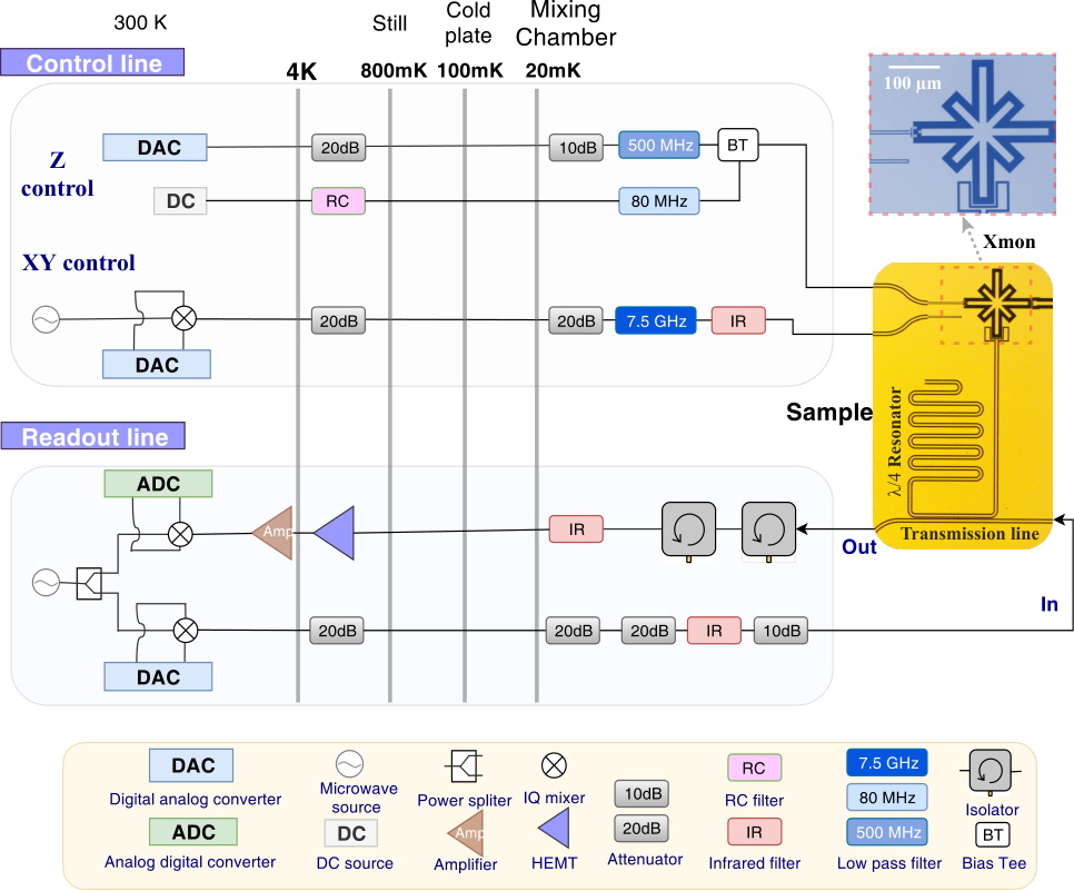
Fig.S7 is the schematic of our experimental setup, showing both wiring scheme and relevant components from room temperature down to the base temperature stages. The samples are mounted in sample boxes made of Al that supply electromagnetic shielding at low temperatures.
The yellow- and blue-shaded areas on the right of Fig.S7 are optical images of one Xmon qubit used in our experiments. Three arms of the cross-shaped capacitance (blue-shaded image) are connected to different elements for coupling to other qubits (right, irrelevant for the current experiment), XY- and Z-control (left), and readout (bottom), respectively. The frequency of the qubit, , is set by the bias on the Z-control line. Microwave pulses in the form of are applied via the XY-control line for various qubit operations. The Xmon qubit is dispersively coupled to a /4 resonator (with a characteristic frequency of ) for readout. More details regarding the design and control of the Xmon-type of qubits, as well as the dispersive readout technique, can be found in Barends2014S; Barends2013S; Kelly2015S; Reed2010S; Sank2016S.
All data of this work, except for those presented in Fig. S4, were obtained from one superconducting Xmon qubit. The qubit frequency is GHz, and the relaxation and dephasing times at this frequency are s and s, respectively. The data in Fig. S4 were acquired on a different qubit with the following parameters: GHz, s and s.
SUPPLEMENTARY REFERENCES
References
- (1) Barends R, Kelly J, Megrant A, et al. Superconducting quantum circuits at the surface code threshold for fault tolerance. Nature 2014; 508:500–503.
- (2) Barends R, Kelly J, Megrant A, et al. Coherent josephson qubit suitable for scalable quantum integrated circuits. Phys Rev Lett 2013; 111:080502.
- (3) Kelly J, Barends R, Fowler AG, et al. State preservation by repetitive error detection in a superconducting quantum circuit. Nature 2015; 519:66–69.
- (4) Reed MD, DiCarlo L, Johnson BR, et al. High-fidelity readout in circuit quantum electrodynamics using the jaynes-cummings nonlinearity. Phys Rev Lett 2010; 105:173601.
- (5) Sank D, Chen Z, Khezri M, et al. Measurement-induced state transitions in a superconducting qubit: Beyond the rotating wave approximation. Phys Rev Lett 2016; 117:190503.