跳到论文正文
W Papers独立论文阅读器 arXiv:2001.03752 论文正文 计算阅读时间 · 0%
引用这篇论文根据当前论文元数据生成,正式投稿前建议核对。


License: arXiv.org perpetual non-exclusive license
arXiv:2001.03752v1 [hep-ph] 11 Jan 2020

Generalized Analysis of the Eötvös Experiment

M. J. Mueterthies Affiliation: Department of Physics and Astronomy, Purdue University, West Lafayette, IN 47907, USA    E. Fischbach Corresponding author: ephraim@purdue.edu Affiliation: Department of Physics and Astronomy, Purdue University, West Lafayette, IN 47907, USA    V. E. Barnes Affiliation: Department of Physics and Astronomy, Purdue University, West Lafayette, IN 47907, USA    J. Bertaux Affiliation: Department of Physics and Astronomy, Purdue University, West Lafayette, IN 47907, USA    D. E. Krause Affiliation: Physics Department, Wabash College, Crawfordsville, IN 47933, USA Affiliation: Department of Physics and Astronomy, Purdue University, West Lafayette, IN 47907, USA    A. Longman Affiliation: Department of Physics and Astronomy, Purdue University, West Lafayette, IN 47907, USA
August 11, 2026
Abstract

We present a generalized phenomenological formalism for analyzing the original Eötvös experiment in the presence of gravity and a generic “5th force.” To date no evidence for a 5th force has emerged since its presence was suggested by a 1986 reanalysis of the 1922 publication coauthored by Eötvös, Pekàr, and Fekete (EPF). However, our generalized analysis introduces new mechanisms capable in principle of accounting for the EPF data, while at the same time avoiding detection by most recent experiments carried out to date. As an example, some of these mechanisms raise the possibility that the EPF signal could have arisen from an unexpected direction if it originated from the motion of the Earth through a medium.

I Introduction

The results of the well-known Eötvös experiment were published in 1922 EPF by Eötvös  Pekàr and Fekete (EPF), following the passing of Eötvös in 1919. The EPF experiment, which was a test of what is now referred to as the weak equivalence principle (WEP), quoted limits on possible WEP violations which were approximately 300 times more sensitive than those from an earlier experiment by Bessel (cited in EPF). However, a 1986 reanalysis of the EPF results Fischbach1986 revealed a pattern in the EPF data which was consistent with the presence of a new interaction coupling to baryon number BB, the so-called “5th force” Fischbach1986. This force was attributed to the virtual exchange of massive vector bosons coupling with fundamental “charge” ff to baryon number BB, giving rise to a two-body potential of the form

V12(r)=f2B1​B2re−r/λ,V_{12}(r)=f^{2}\frac{B_{1}B_{2}}{r}e^{-r/\lambda}, (1)

where λ=ℏ/mb​c\lambda=\hbar/m_{b}c determines the range of the interaction in terms of the boson mass mbm_{b}. Notwithstanding the seemingly compelling evidence for a 5th force that emerged from Ref. Fischbach1986, a force with the characteristics suggested by Ref. Fischbach1986 (a force of intermediate range with roughly gravitational strength) does not appear to be present in nature. (For reviews of the many experiments conducted since 1986, see Refs. Metrologia; FischbachBook; Adelberger2009; Wagner2012; Murata2015).

If we believe that EPF carried out their experiment correctly, and that the subsequent analysis in Ref. Fischbach1986 of the EPF data is also correct, then the failure of the community to detect a 5th force represents a puzzle which has recently been termed the “Eötvös Paradox” Fischbach2019. Specifically, this paradox arises from the mutual incompatibility of the following three statements, each of which appears to be correct Fischbach2019:

  1. 1.

    There is consensus in the community that there were no obvious flaws in the EPF experiment or in the published paper EPF.

  2. 2.

    There is additional consensus that the analysis of the EPF data reported in Ref. Fischbach1986 is also correct, along with its suggestion of a new “5th force” in nature.

  3. 3.

    There is no credible experimental evidence for a new force with the characteristics presented in Ref. Fischbach1986.

Not surprisingly, most attempts to resolve this paradox have focused on the correctness of the EPF experiment. Considerable attention has been devoted to the possibility that some overlooked systematic influences, such as gravity gradients (e.g., Ref. Toth2019), could be responsible for the EPF data. To date, no compelling mechanism has been advanced which accounts for the EPF data in terms of classical environmental effects such as temperature, pressure, or humidity variations, or gravity gradients, etc. (See Ref. Fischbach1988 for an extensive discussion and references and Ref. Volgyesi2019 describing an attempt to repeat the EPF experiment with modern technology.) This is not entirely surprising given that the pattern in the EPF data noted in Ref. Fischbach1986 depends on a non-classical quantity, the baryon-to-mass ratio of each sample (B/μB/\mu in the notation of Ref. Fischbach1986). Further support for the correctness of the EPF experiment comes from a recently discovered handwritten partial draft by Eötvös (autograph) of what would be eventually become the published EPF paper Kilenyi2019. As discussed in Ref. Fischbach2019, this autograph, and various exchanges between Eötvös and Einstein, lend further support to the inference that the EPF experiment was in fact done correctly.

The object of the present paper is to develop a more general phenomenological framework for analyzing the original torsion balance experiment of EPF, and the more modern torsion balance experiments in the presence of both gravity and a possible 5th force. Although the focus of the present paper will be on torsion balance experiments, such as those by the Eöt-Wash collaboration Eotwash1987; Eotwash1988; Eotwash1989, the formalism developed here can be extended to apply to other searches for composition-dependent forces.

The outline of our paper is as follows: In Sec. II we develop the general formalism for combining a composition-independent gravitational interaction with a general composition-dependent interaction arising from a coupling to baryon number BB that lead to a torque on a torsion balance. In Sec. III we apply this formalism to the EPF experiment, taking care to include couplings which were omitted in the original EPF analysis EPF. In Sec. IV, the formalism is then applied to the Eöt-Wash (E-W) experiment of Stubbs, et al. Eotwash1987. In Sec. V, we demonstrate that EPF and E-W experiments are sensitive to different 5th force signals, and in following Sec. VI, we illustrate this using a toy scalar-vector 5th force model. We also consider a qualitatively different scenario to account for the EPF results arising from forces with a non-zero curl. As we note, such forces could arise from a number of sources, including a “magnetic” 5th force, or from a dark matter medium. What is significant about such forces in the present context is that they can appear to arise from unexpected directions, and hence could be rejected as spurious. Since the sensitivity of the E-W experiment (and others) depends to a great extent on knowing the direction from which the presumed 5th force is emanating (such as a nearby mountain), most experiments are optimized to seek a particular signal. Unlike the EPF experiment, more recent force experiments have been designed to set limits on new forces described by potentials similar to Eq. (1). We will suggest, however, that these experiments may not be as sensitive as the EPF experiment to other types of forces.

II General Force acting on a Torsion Balance

In order to determine whether a force exists that could have been detected in the Eötvös experiment, but not in later experiments such as Eöt-Wash, we consider here the response of a mass mm on a torsion balance to a general baryon-number-dependent force F→5\vec{F}_{5}, which we will write in the form of a Taylor expansion about the position of the pivot point R→\vec{R}. Assuming the Einstein summation convention, the iith component of F→5\vec{F}_{5}, F5​iF_{5i}, will be written as

F5​i=ξ​G​m​q​q¯source​[ℱ5​i​(R→)+𝒟5​i​j​(R→)​rj+⋯],F_{5i}=\xi Gmq\overline{q}_{\rm source}\left[\mathcal{F}_{5i}(\vec{R})+\mathcal{D}_{5ij}(\vec{R})r_{j}+\cdots\right], (2)

where ξ\xi is a dimensionless constant, GG is the Newtonian gravitational constant, q=B/μq=B/\mu is the baryon number-to-mass ratio of the sample, q¯source\overline{q}_{\rm source} is the average baryon-to-mass number ratio of the source, and r→\vec{r} is the position of the sample relative to the pivot point. In order for qq and q¯source\overline{q}_{\rm source} to be dimensionless, μ≡m/mH\mu\equiv m/m_{\rm H}, where mH=m(1m_{\rm H}=m(^{1}H)1{}_{1}) is the mass of atomic hydrogen. If F→5\vec{F}_{5} arises from a potential V5=ξ​G​m​q​q¯source​𝒱5V_{5}=\xi Gmq\overline{q}_{\rm source}\mathcal{V}_{5}, then ℱ5​i\mathcal{F}_{5i} is the gradient of 𝒱5\mathcal{V}_{5}, while 𝒟5​i​j\mathcal{D}_{5ij} is the gradient of ℱ5​i\mathcal{F}_{5i}: ℱ5​i=−∂i𝒱5\mathcal{F}_{5i}=-\partial_{i}\mathcal{V}_{5}; 𝒟5​i​j=∂jℱ5​i=−∂i∂j𝒱5\mathcal{D}_{5ij}=\partial_{j}\mathcal{F}_{5i}=-\partial_{i}\partial_{j}\mathcal{V}_{5}, and ∂i=∂/∂Ri\partial_{i}=\partial/\partial R_{i}. To simplify the notation, we introduce

f5​i\displaystyle f_{5i} ≡\displaystyle\equiv ξ​G​q¯source​ℱ5​i,\displaystyle\xi G\overline{q}_{\rm source}\mathcal{F}_{5i}, (3a)
d5​i​j\displaystyle d_{5ij} ≡\displaystyle\equiv ξ​G​q¯source​𝒟5​i​j.\displaystyle\xi G\overline{q}_{\rm source}\mathcal{D}_{5ij}. (3b)

Since both the sources and test masses in torsion balance experiments are extended objects, the 5th force charge will be allowed to vary with position, and hence we replace the mass with the differential mass: m​q→q⁡(r→)​d​m​(r→)mq\rightarrow q(\vec{r})\mathrm{d}m(\vec{r}). The force on the differential element d​m​(r→)\mathrm{d}m(\vec{r}) is then given by

d​F5​i=q⁡(r→)​d​m​(r→)​(f5​i+d5​i​j​rj+⋯).\mathrm{d}F_{5i}=q(\vec{r})\mathrm{d}m(\vec{r})\left(f_{5i}+d_{5ij}r_{j}+\cdots\right). (4)

In addition to the 5th force, the total force F→tot\vec{F}_{\rm tot} will also include the gravitational force F→gravity\vec{F}_{\rm gravity} as well as the centripetal force F→cent\vec{F}_{\rm cent} due to the rotation of the Earth. The iith component of the total force then becomes

Ftot,i=Fgrav,i+Fcent,i+m​q¯​f5​i+m​q¯​ℓ¯j​d5​i​j​,F_{{\rm tot},i}=F_{{\rm grav},i}+F_{{\rm cent},i}+m\overline{q}f_{5i}+m\overline{q}\overline{\ell}_{j}d_{5ij}\text{,} (5)

where m=∫𝑑mm=\int\mathrm{d}m, q¯=∫q⁡(r→)​𝑑m​(r→)/m,\overline{q}=\int q(\vec{r})\,\mathrm{d}m(\vec{r})/m, and ℓ¯j=∫q⁡(r→)​rj​𝑑m​(r→)/m​q¯,\overline{\ell}_{j}=\int q(\vec{r})r_{j}\,\mathrm{d}m(\vec{r})/m\overline{q}, and we have dropped terms higher order in rir_{i}.

To introduce the reference frames relevant to characterize our torsion balance system, we begin with a local North-East-Down (NED) frame as shown in Fig. 1. The forces under consideration are defined in this frame, where the axis of the torsion balance is aligned with the local vertical, found by hanging a plumb bob. The rotation axis b^3\hat{b}_{3} of the torsion balance is then given by

b^3=F→tot|F→tot|,\hat{b}_{3}=\frac{\vec{F}_{\rm tot}}{|\vec{F}_{\rm tot}|}, (6)
Figure 1: Representation of the NED reference frame.

while the b^1\hat{b}_{1}-axis is along the torsion balance beam when the intrinsic twist in the fiber is zero. Since it is convenient for this axis to be roughly towards North (N^\hat{N}), this can be achieved if we define the b^2\hat{b}_{2}-axis, the axis perpendicular to the torsion balance, as

b^2=b^3×N^|b^3×N^|,\hat{b}_{2}=\frac{\hat{b}_{3}\times\hat{N}}{|\hat{b}_{3}\times\hat{N}|}, (7)

and then let b^1\hat{b}_{1} be given by

b^1=b^2×b^3.\hat{b}_{1}=\hat{b}_{2}\times\hat{b}_{3}. (8)

The b^\hat{b} frame is space-fixed in the zero-twist orientation of the beam and makes an angle β\beta with the NED frame as shown in Fig. 2). If F→tot\vec{F}_{\rm tot} were directed downward, β=0\beta=0 and the NED and b^\hat{b} frames would coincide.

We also introduce the body fixed xx-yy-zz frame which is a rotation of the b^\hat{b} frame by the angle θ\theta,

N^\displaystyle\hat{N} =\displaystyle= x^​cϕ​cβ−y^​sϕ​cβ−z^​sβ,\displaystyle\hat{x}c_{\phi}c_{\beta}-\hat{y}s_{\phi}c_{\beta}-\hat{z}s_{\beta}, (9a)
E^\displaystyle\hat{E} =\displaystyle= x^​sϕ+y^​cϕ,\displaystyle\hat{x}s_{\phi}+\hat{y}c_{\phi}, (9b)
D^\displaystyle\hat{D} =\displaystyle= x^​cϕ​sβ−y^​sϕ​sβ+z^​cβ.\displaystyle\hat{x}c_{\phi}s_{\beta}-\hat{y}s_{\phi}s_{\beta}+\hat{z}c_{\beta}. (9c)

Here and throughout the rest of the text, we use the notation

cϕ\displaystyle c_{\phi} ≡\displaystyle\equiv cos⁡ϕ,\displaystyle\cos\phi, (10a)
sϕ\displaystyle s_{\phi} ≡\displaystyle\equiv sin⁡ϕ,\displaystyle\sin\phi, (10b)

and similar expressions for angles β\beta, etc. The frame relations are also depicted in Figure 2.
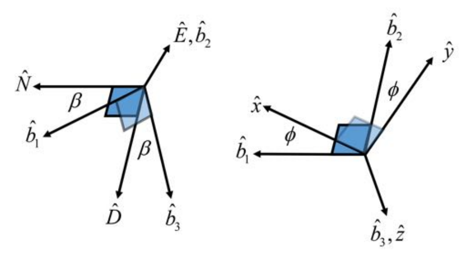
Refer to caption
Figure 2: The transformations from the NED frame to the body frame.

To find the torque on the torsion balance, we use the Lagrangian formulation

dd​t​(∂ℒ∂ϕ˙)−∂ℒ∂ϕ=Q5​ϕ​,\frac{\mathrm{d}}{\mathrm{d}t}\left(\frac{\partial\mathcal{L}}{\partial\dot{\phi}}\right)-\frac{\partial\mathcal{L}}{\partial\phi}=Q_{5\phi}\text{,} (11)

where Q5​ϕQ_{5\phi} is the generalized 5th force given by,

d​Q5​ϕ\displaystyle\mathrm{d}Q_{5\phi} =\displaystyle= ∂ri∂ϕ⋅d​ℱ5​i\displaystyle\frac{\partial r_{i}}{\partial\phi}\cdot\mathrm{d}\mathcal{F}_{5i} (12)
=\displaystyle= q⁡(r→)​d​m​(r→)​(f5​i​∂ri∂ϕ+d5​i​j​rj​∂ri∂ϕ)\displaystyle q(\vec{r})\mathrm{d}m(\vec{r})\left(f_{5i}\frac{\partial r_{i}}{\partial\phi}+d_{5ij}r_{j}\frac{\partial r_{i}}{\partial\phi}\right)
=\displaystyle= q⁡(r→)​ρ​(r→)​d​V​(f5​i​∂ri∂ϕ+d5​i​j​rj​∂ri∂ϕ)​.\displaystyle q(\vec{r})\rho(\vec{r})\mathrm{d}V\left(f_{5i}\frac{\partial r_{i}}{\partial\phi}+d_{5ij}r_{j}\frac{\partial r_{i}}{\partial\phi}\right)\text{.}

We note that r→\vec{r} here, and in Eq. (2), is the position of the particle in the NED frame, which can be written as

r→\displaystyle\vec{r} =\displaystyle= x​x^+y​y^+z​z^\displaystyle x\hat{x}+y\hat{y}+z\hat{z} (13)
=\displaystyle= (x​cϕ​cβ−y​sϕ​cβ−z​sβ)​N^+(x​sϕ+y​cϕ)​E^\displaystyle\left(xc_{\phi}c_{\beta}-ys_{\phi}c_{\beta}-zs_{\beta}\right)\hat{N}+\left(xs_{\phi}+yc_{\phi}\right)\hat{E}
+(x​cϕ​sβ−y​sϕ​sβ+z​cβ)​D^​.\displaystyle+\left(xc_{\phi}s_{\beta}-ys_{\phi}s_{\beta}+zc_{\beta}\right)\hat{D}\text{.}

It is straightforward to show that the angular derivative of r→\vec{r} is

∂r→∂ϕ=(−x​sϕ​cβ−y​cϕ​cβ)​N^+(x​cϕ−y​sϕ)​E^+(−x​sϕ​sβ−y​cϕ​sβ)​D^​.\frac{\partial\vec{r}}{\partial\phi}=\left(-xs_{\phi}c_{\beta}-yc_{\phi}c_{\beta}\right)\hat{N}+\left(xc_{\phi}-ys_{\phi}\right)\hat{E}+\left(-xs_{\phi}s_{\beta}-yc_{\phi}s_{\beta}\right)\hat{D}\text{.} (14)

III Application to the EPF Experiment

Table 1: Notation correspondence between EPF (Ref. EPF) and this work.
This work EPF Description
II KK Moment of Inertia
VgravV_{\rm grav} −U-U Gravitational Potential Energy
δ\delta LL Observation scale length
LL ℓa\ell_{a} Torsion Balance length
mm MaM_{a} Sample mass
β\beta ϵ\epsilon Plumb bob angle
Δ​ϕ\Delta\phi Δ​α\Delta\alpha Intrinsic twist of the wire
σ\sigma m=nE−nWm=n_{E}-n_{W} East-West observation difference

To be more consistent with current practices, we have modified the notation of Ref. EPF as shown in Table 1. The EPF experiment compared two masses, as shown in Fig. 3. Mass 1 was located along the balance towards North and hung a distance hh below the balance. Mass 2 was located along the balance towards the South and was located at the same height as the balance.

Figure 3: Side view of the Eötvös Experiment.
Figure 4: Top view of the Eötvös Experiment.

The product of the 5th force charge and the mass density of the EPF samples can be written as,

q⁡(r→)​ρ​(r→)=q1​δ​(x−L)​δ​(y)​δ​(z−h)+q2​δ​(x+L)​δ​(y)​δ​(z)​.q\left(\vec{r}\right)\rho\left(\vec{r}\right)=q_{1}\delta\left(x-L\right)\delta\left(y\right)\delta\left(z-h\right)+q_{2}\delta\left(x+L\right)\delta\left(y\right)\delta\left(z\right)\text{.} (15)

Using Eq. (15), the torque on the fiber can then be expressed in the form

T5\displaystyle T_{5} =\displaystyle= −(q1−q2)​m​L​cβ​sϕ​f5​x+(q1−q2)​m​L​cϕ​f5​y−(q1−q2)​m​L​sβ​sϕ​f5​z\displaystyle-(q_{1}-q_{2})mLc_{\beta}s_{\phi}f_{5x}+(q_{1}-q_{2})mLc_{\phi}f_{5y}-(q_{1}-q_{2})mLs_{\beta}s_{\phi}f_{5z} (16)
−(q1+q2)​I2​cβ2​cϕ​sϕ​d5​x​x+q1​m​L​h​sβ​cβ​sϕ​d5​x​x\displaystyle-(q_{1}+q_{2})\frac{I}{2}c_{\beta}^{2}c_{\phi}s_{\phi}d_{5xx}+q_{1}mLhs_{\beta}c_{\beta}s_{\phi}d_{5xx}
+(q1+q2)​I2​cβ​cϕ2​d5​y​x−q1​m​L​h​sβ​cϕ​d5​y​x\displaystyle+(q_{1}+q_{2})\frac{I}{2}c_{\beta}c_{\phi}^{2}d_{5yx}-q_{1}mLhs_{\beta}c_{\phi}d_{5yx}
−(q1+q2)​I2​cβ​sβ​cϕ​sϕ​d5​z​x+q1​m​L​h​sβ2​sϕ​d5​z​x\displaystyle-(q_{1}+q_{2})\frac{I}{2}c_{\beta}s_{\beta}c_{\phi}s_{\phi}d_{5zx}+q_{1}mLhs_{\beta}^{2}s_{\phi}d_{5zx}
−(q1+q2)​I2​cβ​sϕ2​d5​x​y+(q1+q2)​I2​cϕ​sϕ​d5​y​y−(q1+q2)​I2​sβ​sϕ2​d5​z​y\displaystyle-(q_{1}+q_{2})\frac{I}{2}c_{\beta}s_{\phi}^{2}d_{5xy}+(q_{1}+q_{2})\frac{I}{2}c_{\phi}s_{\phi}d_{5yy}-(q_{1}+q_{2})\frac{I}{2}s_{\beta}s_{\phi}^{2}d_{5zy}
−(q1+q2)​I2​cβ​sβ​cϕ​sϕ​d5​x​z−q1​m​L​h​cβ2​sϕ​d5​x​z\displaystyle-(q_{1}+q_{2})\frac{I}{2}c_{\beta}s_{\beta}c_{\phi}s_{\phi}d_{5xz}-q_{1}mLhc_{\beta}^{2}s_{\phi}d_{5xz}
+(q1+q2)​I2​sβ​cϕ2​d5​y​z+q1​m​L​h​cβ​cϕ​d5​y​z\displaystyle+(q_{1}+q_{2})\frac{I}{2}s_{\beta}c_{\phi}^{2}d_{5yz}+q_{1}mLhc_{\beta}c_{\phi}d_{5yz}
−(q1+q2)​I2​sβ2​cϕ​sϕ​d5​z​z−q1​m​L​h​sβ​cβ​sϕ​d5​z​z​.\displaystyle-(q_{1}+q_{2})\frac{I}{2}s_{\beta}^{2}c_{\phi}s_{\phi}d_{5zz}-q_{1}mLhs_{\beta}c_{\beta}s_{\phi}d_{5zz}\text{.}

We also need the gravitational and centrifugal force vectors, which can be determined in two ways. First, we could form the Lagrangian using the gravitational potential energy and the effective potential energy for the centrifugal force. Then we expand the Lagrangian to second order in r→\vec{r}, and finally apply Eq. (11) to find the torque. Alternatively, we can use the results from Eq. (16) to quickly deduce the remaining terms, as Eq. (16) was written generically. We simply let q1=q2=1q_{1}=q_{2}=1, fi=−∂iVgrav+Fcent,i/mf_{i}=-\partial_{i}V_{\rm grav}+F_{{\rm cent},i}/m, and di​j=−∂i∂jVgravd_{ij}=-\partial_{i}\partial_{j}V_{\rm grav}, where VgravV_{\rm grav} is the gravitational potential and Fcent,iF_{{\rm cent},i} is the iith component of the centrifugal force. The Newtonian contribution to the torque is then given,

Tgrav\displaystyle T_{\rm grav} =\displaystyle= I​cβ2​cϕ​sϕ​∂x2Vgrav−m​L​h​sβ​cβ​sϕ​∂x2Vgrav−I​cβ​(cϕ2−sϕ2)​∂x∂yVgrav\displaystyle Ic_{\beta}^{2}c_{\phi}s_{\phi}\partial_{x}^{2}V_{\rm grav}-mLhs_{\beta}c_{\beta}s_{\phi}\partial_{x}^{2}V_{\rm grav}-Ic_{\beta}(c_{\phi}^{2}-s_{\phi}^{2})\partial_{x}\partial_{y}V_{\rm grav} (17)
+mLhsβcϕ∂x∂yVgrav+2Icβsβcϕsϕ∂x∂zVgrav+mLh(cβ2\displaystyle+mLhs_{\beta}c_{\phi}\partial_{x}\partial_{y}V_{\rm grav}+2Ic_{\beta}s_{\beta}c_{\phi}s_{\phi}\partial_{x}\partial_{z}V_{\rm grav}+mLh(c_{\beta}^{2}
OPEN−sβ2)​sϕ​∂x∂zVgrav−I​cϕ​sϕ​∂y2Vgrav−I​sβ​(cϕ2−sϕ2)​∂y∂zVgrav\displaystyle-s_{\beta}^{2})s_{\phi}\partial_{x}\partial_{z}V_{\rm grav}-Ic_{\phi}s_{\phi}\partial_{y}^{2}V_{\rm grav}-Is_{\beta}(c_{\phi}^{2}-s_{\phi}^{2})\partial_{y}\partial_{z}V_{\rm grav}
−mLcβcϕ∂y∂zVgrav+Isβ2cϕsϕ∂z2Vgrav+mLhsβcβsϕ∂z2Vgrav.\displaystyle-mLc_{\beta}c_{\phi}\partial_{y}\partial_{z}V_{\rm grav}+Is_{\beta}^{2}c_{\phi}s_{\phi}\partial_{z}^{2}V_{\rm grav}+mLhs_{\beta}c_{\beta}s_{\phi}\partial_{z}^{2}V_{\rm grav}\text{.}

When β\beta and sβs_{\beta} are small, so that cβ≈1c_{\beta}\approx 1, the gravitational terms simplify to

Tgrav\displaystyle T_{\rm grav} ≈\displaystyle\approx [−I(∂y2Vgrav−∂x2Vgrav)s2​ϕ2−I∂x∂yVgravc2​ϕ\displaystyle\biggl[-I(\partial_{y}^{2}V_{\rm grav}-\partial_{x}^{2}V_{\rm grav})\frac{s_{2\phi}}{2}-I\partial_{x}\partial_{y}V_{\rm grav}c_{2\phi} (18)
+mLh∂x∂zVgravsϕ−mLh∂y∂zVgravcϕ]\displaystyle+mLh\partial_{x}\partial_{z}V_{\rm grav}s_{\phi}-mLh\partial_{y}\partial_{z}V_{\rm grav}c_{\phi}\biggr]
−I∂y∂zVgravsβc2​ϕ+mLh∂x∂yVgravsβcϕ\displaystyle-I\partial_{y}\partial_{z}V_{\rm grav}s_{\beta}c_{2\phi}+mLh\partial_{x}\partial_{y}V_{\rm grav}s_{\beta}c_{\phi}
−mLh∂x2Vgravsβsϕ+I∂x∂zVgravsβs2​ϕ\displaystyle-mLh\partial_{x}^{2}V_{\rm grav}s_{\beta}s_{\phi}+I\partial_{x}\partial_{z}V_{\rm grav}s_{\beta}s_{2\phi}
+mLh∂z2Vgravsβsϕ.\displaystyle+mLh\partial_{z}^{2}V_{\rm grav}s_{\beta}s_{\phi}.

The first five terms (in square brackets) reproduce those of EPF EPF (up to a sign), while the remaining five terms do not appear in EPF, since they contain sβs_{\beta} multiplied by gravity gradients which EPF neglected.

The total torque can then be written as

Ttotal\displaystyle T_{\rm total} =\displaystyle= [−I(∂y2Vgrav−∂x2Vgrav)s2​ϕ2−I∂x∂yVgravc2​ϕ\displaystyle\biggr[-I(\partial_{y}^{2}V_{\rm grav}-\partial_{x}^{2}V_{\rm grav})\frac{s_{2\phi}}{2}-I\partial_{x}\partial_{y}V_{\rm grav}c_{2\phi} (19)
+mLh∂x∂zVgravsϕ−mLh∂y∂zVgravcϕ]EPF\displaystyle+mLh\partial_{x}\partial_{z}V_{\rm grav}s_{\phi}-mLh\partial_{y}\partial_{z}V_{\rm grav}c_{\phi}\biggl]_{\text{EPF}}
+[q+I4(d5​y​y−d5​x​x)s2​ϕ+q+I4(d5​y​x+d5​x​y)c2​ϕ\displaystyle+\biggr[q_{+}\frac{I}{4}\left(d_{5yy}-d_{5xx}\right)s_{2\phi}+q_{+}\frac{I}{4}\left(d_{5yx}+d_{5xy}\right)c_{2\phi}
−q1​m​L​h​d5​x​z​sϕ+q1​m​L​h​d5​y​z​cϕ−q−​m​L​f5​z​sβ​sϕ\displaystyle-q_{1}mLhd_{5xz}s_{\phi}+q_{1}mLhd_{5yz}c_{\phi}-q_{-}mLf_{5z}s_{\beta}s_{\phi}
+q+​I4​(d5​y​z+d5​z​y)​sβ​c2​ϕ−q1​m​L​h​d5​y​x​sβ​cϕ\displaystyle+q_{+}\frac{I}{4}\left(d_{5yz}+d_{5zy}\right)s_{\beta}c_{2\phi}-q_{1}mLhd_{5yx}s_{\beta}c_{\phi}
+q1​m​L​h​d5​x​x​sβ​sϕ−q+​I4​(d5​x​z+d5​z​x)​sβ​s2​ϕ\displaystyle+q_{1}mLhd_{5xx}s_{\beta}s_{\phi}-q_{+}\frac{I}{4}\left(d_{5xz}+d_{5zx}\right)s_{\beta}s_{2\phi}
−q1mLhsβsϕd5​z​z]EPF+\displaystyle-q_{1}mLhs_{\beta}s_{\phi}d_{5zz}\biggr]_{\text{EPF+}}
+[−q−mLf5​xsϕ+q−mLf5​ycϕ]EPFx\displaystyle+\biggr[-q_{-}mLf_{5x}s_{\phi}+q_{-}mLf_{5y}c_{\phi}\biggr]_{\text{EPFx}}
+[q+I4(d5​y​x−d5​x​y)+q+I4(d5​y​z−d5​z​y)sβ]NZC.\displaystyle+\biggl[q_{+}\frac{I}{4}\left(d_{5yx}-d_{5xy}\right)+q_{+}\frac{I}{4}\left(d_{5yz}-d_{5zy}\right)s_{\beta}\biggl]_{\text{NZC}}\text{.}

To more easily compare our results to those of EPF, we adopt a convention where in the first set of square brackets, []EPF[\ ]_{\text{EPF}}, are those terms that appear in Eq. (8) of Ref. EPF (the gravity gradient terms). These are followed by our three new “non-EPF” terms: In Eq. (19), the []EPF+[\ ]_{\text{EPF+}} terms are the 5th-force equivalents to the gravity gradients. The []EPF+[\ ]_{\text{EPF+}} terms should reduce to the []EPF[\ ]_{\text{EPF}} terms if the 5th force is replaced by the gravitational force. The []EPFx[\ ]_{\text{EPFx}} terms are entirely new (xx and yy direction forces), and the []NZC[\ ]_{\text{NZC}} terms are only relevant if the 5th force has a nonzero curl. Such terms can arise from the interactions of the test samples with a medium, and thus represent a possible new mechanism which might account for the EPF results.

We now introduce the scale value nn, the constant n0n_{0}, the length LL, and the torsion constant τ\tau of the wire and write the torque as

Ttotal=τ​n0−n2​δ​.T_{\rm total}=\tau\frac{n_{0}-n}{2\delta}\text{.} (20)

The measured quantity is then

n0−n\displaystyle n_{0}-n =\displaystyle= [−δτI(∂y2Vgrav−∂x2Vgrav)s2​ϕ−2​δτI∂x∂yVgravc2​ϕ\displaystyle\biggl[-\frac{\delta}{\tau}I(\partial_{y}^{2}V_{\rm grav}-\partial_{x}^{2}V_{\rm grav})s_{2\phi}-\frac{2\delta}{\tau}I\partial_{x}\partial_{y}V_{\rm grav}c_{2\phi} (21)
+2​δτmLh∂x∂zVgravsϕ−2​δτmLh∂y∂zVgravcϕ]EPF\displaystyle+\frac{2\delta}{\tau}mLh\partial_{x}\partial_{z}V_{\rm grav}s_{\phi}-\frac{2\delta}{\tau}mLh\partial_{y}\partial_{z}V_{\rm grav}c_{\phi}\biggr]_{\text{EPF}}
+[q+δτI2(d5​y​y−d5​x​x)s2​ϕ+q+δτI2(d5​y​x+d5​x​y)c2​ϕ\displaystyle+\biggl[q_{+}\frac{\delta}{\tau}\frac{I}{2}\left(d_{5yy}-d_{5xx}\right)s_{2\phi}+q_{+}\frac{\delta}{\tau}\frac{I}{2}\left(d_{5yx}+d_{5xy}\right)c_{2\phi}
−q1​2​δτ​m​L​h​d5​x​z​sϕ+q1​2​δτ​m​L​h​d5​y​z​cϕ−q−​2​δτ​m​L​f5​z​sβ​sϕ\displaystyle-q_{1}\frac{2\delta}{\tau}mLhd_{5xz}s_{\phi}+q_{1}\frac{2\delta}{\tau}mLhd_{5yz}c_{\phi}-q_{-}\frac{2\delta}{\tau}mLf_{5z}s_{\beta}s_{\phi}
+q+​δτ​I2​(d5​y​z+d5​z​y)​sβ​c2​ϕ−q1​2​δτ​m​L​h​d5​y​x​sβ​cϕ\displaystyle+q_{+}\frac{\delta}{\tau}\frac{I}{2}\left(d_{5yz}+d_{5zy}\right)s_{\beta}c_{2\phi}-q_{1}\frac{2\delta}{\tau}mLhd_{5yx}s_{\beta}c_{\phi}
+q1​2​δτ​m​L​h​d5​x​x​sβ​sϕ−q+​δτ​I2​(d5​x​z+d5​z​x)​sβ​s2​ϕ\displaystyle+q_{1}\frac{2\delta}{\tau}mLhd_{5xx}s_{\beta}s_{\phi}-q_{+}\frac{\delta}{\tau}\frac{I}{2}\left(d_{5xz}+d_{5zx}\right)s_{\beta}s_{2\phi}
−q12​δτmLhd5​z​zsβsϕ]EPF+\displaystyle-q_{1}\frac{2\delta}{\tau}mLhd_{5zz}s_{\beta}s_{\phi}\biggr]_{\text{EPF+}}
+[−q−​2​δτ​m​L​f5​x​sϕ+q−​2​δτ​m​L​f5​y​cϕ]EPFx\displaystyle+\biggl[-q_{-}\frac{2\delta}{\tau}mLf_{5x}s_{\phi}+q_{-}\frac{2\delta}{\tau}mLf_{5y}c_{\phi}\biggr]_{\text{EPFx}}
+[q+​δτ​I2​(d5​y​x−d5​x​y)+q+​δτ​I2​(d5​y​z−d5​z​y)​sβ]NZC​.\displaystyle+\biggl[q_{+}\frac{\delta}{\tau}\frac{I}{2}\left(d_{5yx}-d_{5xy}\right)+q_{+}\frac{\delta}{\tau}\frac{I}{2}\left(d_{5yz}-d_{5zy}\right)s_{\beta}\biggr]_{\text{NZC}}\text{.}

EPF measured the scale value in four orientations: North (N), East (E), South (S), and West (W). When the apparatus is pointed toward the North, the deflection of the balance from North is simply due to the intrinsic twist Δ​ϕ\Delta\phi in the wire. Thus,

ϕN\displaystyle\phi_{N} =\displaystyle= Δ​ϕ​,\displaystyle\Delta\phi\text{,} (22a)
sϕN\displaystyle s_{\phi_{N}} =\displaystyle= Δ​ϕ​,\displaystyle\Delta\phi\text{,} (22b)
s2​ϕN\displaystyle s_{2\phi_{N}} =\displaystyle= 2​Δ​ϕ​,\displaystyle 2\Delta\phi\text{,} (22c)
cϕN\displaystyle c_{\phi_{N}} =\displaystyle= 1​,\displaystyle 1\text{,} (22d)
c2​ϕN\displaystyle c_{2\phi_{N}} =\displaystyle= 1​.\displaystyle 1\text{.} (22e)

Then,

n0−nN\displaystyle n_{0}-n_{N} =\displaystyle= [−2​δτI(∂y2Vgrav−∂x2Vgrav)Δϕ−2​δτI∂x∂yVgrav\displaystyle\biggl[-\frac{2\delta}{\tau}I(\partial_{y}^{2}V_{\rm grav}-\partial_{x}^{2}V_{\rm grav})\Delta\phi-\frac{2\delta}{\tau}I\partial_{x}\partial_{y}V_{\rm grav} (23)
+2​δτmLh∂x∂zVgravΔϕ−2​δτmLh∂y∂zVgrav]EPF\displaystyle+\frac{2\delta}{\tau}mLh\partial_{x}\partial_{z}V_{\rm grav}\Delta\phi-\frac{2\delta}{\tau}mLh\partial_{y}\partial_{z}V_{\rm grav}\biggr]_{\text{EPF}}
+[q+δτI(d5​y​y−d5​x​x)Δϕ+q+δτId5​y​x\displaystyle+\biggr[q_{+}\frac{\delta}{\tau}I\left(d_{5yy}-d_{5xx}\right)\Delta\phi+q_{+}\frac{\delta}{\tau}Id_{5yx}
−q1​2​δτ​m​L​h​d5​x​z​Δ​ϕ+q1​2​δτ​m​L​h​d5​y​z\displaystyle-q_{1}\frac{2\delta}{\tau}mLhd_{5xz}\Delta\phi+q_{1}\frac{2\delta}{\tau}mLhd_{5yz}
+q+δτId5​y​zsβ−q12​δτmLhd5​y​xsβ]EPF+\displaystyle+q_{+}\frac{\delta}{\tau}Id_{5yz}s_{\beta}-q_{1}\frac{2\delta}{\tau}mLhd_{5yx}s_{\beta}\biggr]_{\text{EPF+}}
+[−q−​2​δτ​m​L​f5​x​Δ​ϕ+q−​2​δτ​m​L​f5​y]EPFx​.\displaystyle+\biggl[-q_{-}\frac{2\delta}{\tau}mLf_{5x}\Delta\phi+q_{-}\frac{2\delta}{\tau}mLf_{5y}\biggr]_{\text{EPFx}}\text{.}

When the apparatus is pointed in the Eastern direction, the deflection of the beam balance from North is due to a combination of the intrinsic twist, the difference in the measurements nNn_{N} and nEn_{E}, and a factor of π/2\pi/2 due to physically rotating the balance. Thus

ϕE\displaystyle\phi_{E} =\displaystyle= Δ​ϕ+nN−nE2​δ+π2​,\displaystyle\Delta\phi+\frac{n_{N}-n_{E}}{2\delta}+\frac{\pi}{2}\text{,} (24a)
sϕE\displaystyle s_{\phi_{E}} =\displaystyle= 1​,\displaystyle 1\text{,} (24b)
s2​ϕE\displaystyle s_{2\phi_{E}} =\displaystyle= −2​(Δ​ϕ+nN−nE2​δ)​,\displaystyle-2\left(\Delta\phi+\frac{n_{N}-n_{E}}{2\delta}\right)\text{,} (24c)
cϕE\displaystyle c_{\phi_{E}} =\displaystyle= −(Δ​ϕ+nN−nE2​δ)​,\displaystyle-\left(\Delta\phi+\frac{n_{N}-n_{E}}{2\delta}\right)\text{,} (24d)
c2​ϕE\displaystyle c_{2\phi_{E}} =\displaystyle= −1​,\displaystyle-1\text{,} (24e)
n0−nE\displaystyle n_{0}-n_{E} =\displaystyle= [2​δτI(∂y2Vgrav−∂x2Vgrav)(Δϕ+nN−nE2​δ)+2​δτI∂x∂yVgrav\displaystyle\biggl[\frac{2\delta}{\tau}I(\partial_{y}^{2}V_{\rm grav}-\partial_{x}^{2}V_{\rm grav})\left(\Delta\phi+\frac{n_{N}-n_{E}}{2\delta}\right)+\frac{2\delta}{\tau}I\partial_{x}\partial_{y}V_{\rm grav} (25)
+2​δτmLh∂x∂zVgrav+2​δτmLh∂y∂zVgrav(Δϕ+nN−nE2​δ)]EPF\displaystyle+\frac{2\delta}{\tau}mLh\partial_{x}\partial_{z}V_{\rm grav}+\frac{2\delta}{\tau}mLh\partial_{y}\partial_{z}V_{\rm grav}\left(\Delta\phi+\frac{n_{N}-n_{E}}{2\delta}\right)\biggr]_{\text{EPF}}
+[−q+δτI(d5​y​y−d5​x​x)(Δϕ+nN−nE2​δ)−q+δτId5​x​y\displaystyle+\biggl[-q_{+}\frac{\delta}{\tau}I\left(d_{5yy}-d_{5xx}\right)\left(\Delta\phi+\frac{n_{N}-n_{E}}{2\delta}\right)-q_{+}\frac{\delta}{\tau}Id_{5xy}
−q1​2​δτ​m​L​h​d5​x​z−q1​2​δτ​m​L​h​d5​y​z​(Δ​ϕ+nN−nE2​δ)\displaystyle-q_{1}\frac{2\delta}{\tau}mLhd_{5xz}-q_{1}\frac{2\delta}{\tau}mLhd_{5yz}\left(\Delta\phi+\frac{n_{N}-n_{E}}{2\delta}\right)
−q−​2​δτ​m​L​f5​z​sβ−q+​δτ​I​d5​z​y​sβ\displaystyle-q_{-}\frac{2\delta}{\tau}mLf_{5z}s_{\beta}-q_{+}\frac{\delta}{\tau}Id_{5zy}s_{\beta}
+q12​δτmLhd5​x​xsβ−q12​δτmLhd5​z​zsβ]EPF+\displaystyle+q_{1}\frac{2\delta}{\tau}mLhd_{5xx}s_{\beta}-q_{1}\frac{2\delta}{\tau}mLhd_{5zz}s_{\beta}\biggr]_{\text{EPF+}}
+[−q−​2​δτ​m​L​f5​x−q−​2​δτ​m​L​f5​y​(Δ​ϕ+nN−nE2​δ)]EPFx​.\displaystyle+\biggl[-q_{-}\frac{2\delta}{\tau}mLf_{5x}-q_{-}\frac{2\delta}{\tau}mLf_{5y}\left(\Delta\phi+\frac{n_{N}-n_{E}}{2\delta}\right)\biggr]_{\text{EPFx}}\text{.}

Rotating the apparatus to point in the Southern direction yields

ϕS\displaystyle\phi_{S} =\displaystyle= Δ​ϕ+nN−nS2​δ+π​,\displaystyle\Delta\phi+\frac{n_{N}-n_{S}}{2\delta}+\pi\text{,} (26a)
sϕS\displaystyle s_{\phi_{S}} =\displaystyle= −(Δ​ϕ+nN−nS2​δ)​,\displaystyle-\left(\Delta\phi+\frac{n_{N}-n_{S}}{2\delta}\right)\text{,} (26b)
s2​ϕS\displaystyle s_{2\phi_{S}} =\displaystyle= 2​(Δ​ϕ+nN−nS2​δ)​,\displaystyle 2\left(\Delta\phi+\frac{n_{N}-n_{S}}{2\delta}\right)\text{,} (26c)
cϕS\displaystyle c_{\phi_{S}} =\displaystyle= −1​,\displaystyle-1\text{,} (26d)
c2​ϕS\displaystyle c_{2\phi_{S}} =\displaystyle= 1​,\displaystyle 1\text{,} (26e)

and,

n0−nS\displaystyle n_{0}-n_{S} =\displaystyle= [−2​δτI(∂y2Vgrav−∂x2Vgrav)(Δϕ+nN−nS2​δ)−2​δτI∂x∂yVgrav\displaystyle\biggl[-\frac{2\delta}{\tau}I(\partial_{y}^{2}V_{\rm grav}-\partial_{x}^{2}V_{\rm grav})\left(\Delta\phi+\frac{n_{N}-n_{S}}{2\delta}\right)-\frac{2\delta}{\tau}I\partial_{x}\partial_{y}V_{\rm grav} (27)
−2​δτmLh∂x∂zVgrav(Δϕ+nN−nS2​δ)+2​δτmLh∂y∂zVgrav]EPF\displaystyle-\frac{2\delta}{\tau}mLh\partial_{x}\partial_{z}V_{\rm grav}\left(\Delta\phi+\frac{n_{N}-n_{S}}{2\delta}\right)+\frac{2\delta}{\tau}mLh\partial_{y}\partial_{z}V_{\rm grav}\biggr]_{\text{EPF}}
[+q+δτI(d5​y​y−d5​x​x)(Δϕ+nN−nS2​δ)+q+δτId5​y​x\displaystyle\biggl[+q_{+}\frac{\delta}{\tau}I\left(d_{5yy}-d_{5xx}\right)\left(\Delta\phi+\frac{n_{N}-n_{S}}{2\delta}\right)+q_{+}\frac{\delta}{\tau}Id_{5yx}
+q1​2​δτ​m​L​h​d5​x​z​(Δ​ϕ+nN−nS2​δ)−q1​2​δτ​m​L​h​d5​y​z\displaystyle+q_{1}\frac{2\delta}{\tau}mLhd_{5xz}\left(\Delta\phi+\frac{n_{N}-n_{S}}{2\delta}\right)-q_{1}\frac{2\delta}{\tau}mLhd_{5yz}
+q+δτId5​y​zsβ+q12​δτmLhd5​y​xsβ]EPF+\displaystyle+q_{+}\frac{\delta}{\tau}Id_{5yz}s_{\beta}+q_{1}\frac{2\delta}{\tau}mLhd_{5yx}s_{\beta}\biggr]_{\text{EPF+}}
+[q−​2​δτ​m​L​f5​x​(Δ​ϕ+nN−nS2​δ)−q−​2​δτ​m​L​f5​y]EPFx​.\displaystyle+\biggl[q_{-}\frac{2\delta}{\tau}mLf_{5x}\left(\Delta\phi+\frac{n_{N}-n_{S}}{2\delta}\right)-q_{-}\frac{2\delta}{\tau}mLf_{5y}\biggr]_{\text{EPFx}}\text{.}

Finally, rotating the apparatus to point in the Western direction yields

ϕW\displaystyle\phi_{W} =\displaystyle= Δ​ϕ+nN−nW2​δ+3​π2​,\displaystyle\Delta\phi+\frac{n_{N}-n_{W}}{2\delta}+\frac{3\pi}{2}\text{,} (28a)
sϕW\displaystyle s_{\phi_{W}} =\displaystyle= −1​,\displaystyle-1\text{,} (28b)
s2​ϕW\displaystyle s_{2\phi_{W}} =\displaystyle= −2​(Δ​ϕ+nN−nW2​δ)​,\displaystyle-2\left(\Delta\phi+\frac{n_{N}-n_{W}}{2\delta}\right)\text{,} (28c)
cϕW\displaystyle c_{\phi_{W}} =\displaystyle= (Δ​ϕ+nN−nW2​δ)​,\displaystyle\left(\Delta\phi+\frac{n_{N}-n_{W}}{2\delta}\right)\text{,} (28d)
c2​ϕW\displaystyle c_{2\phi_{W}} =\displaystyle= −1​,\displaystyle-1\text{,} (28e)

and,

n0−nW\displaystyle n_{0}-n_{W} =\displaystyle= [2​δτI(∂y2Vgrav−∂x2Vgrav)(Δϕ+nN−nW2​δ)+2​δτI∂x∂yVgrav\displaystyle\biggl[\frac{2\delta}{\tau}I(\partial_{y}^{2}V_{\rm grav}-\partial_{x}^{2}V_{\rm grav})\left(\Delta\phi+\frac{n_{N}-n_{W}}{2\delta}\right)+\frac{2\delta}{\tau}I\partial_{x}\partial_{y}V_{\rm grav} (29)
−2​δτmLh∂x∂zVgrav−2​δτmLh∂y∂zVgrav(Δϕ+nN−nW2​δ)]EPF\displaystyle-\frac{2\delta}{\tau}mLh\partial_{x}\partial_{z}V_{\rm grav}-\frac{2\delta}{\tau}mLh\partial_{y}\partial_{z}V_{\rm grav}\left(\Delta\phi+\frac{n_{N}-n_{W}}{2\delta}\right)\biggr]_{\text{EPF}}
+[−q+δτI(d5​y​y−d5​x​x)(Δϕ+nN−nW2​δ)−q+δτId5​x​y\displaystyle+\biggl[-q_{+}\frac{\delta}{\tau}I\left(d_{5yy}-d_{5xx}\right)\left(\Delta\phi+\frac{n_{N}-n_{W}}{2\delta}\right)-q_{+}\frac{\delta}{\tau}Id_{5xy}
+q1​2​δτ​m​L​h​d5​x​z+q1​2​δτ​m​L​h​d5​y​z​(Δ​ϕ+nN−nW2​δ)\displaystyle+q_{1}\frac{2\delta}{\tau}mLhd_{5xz}+q_{1}\frac{2\delta}{\tau}mLhd_{5yz}\left(\Delta\phi+\frac{n_{N}-n_{W}}{2\delta}\right)
+q−​2​δτ​m​L​f5​z​sβ−q+​δτ​I​d5​z​y​sβ\displaystyle+q_{-}\frac{2\delta}{\tau}mLf_{5z}s_{\beta}-q_{+}\frac{\delta}{\tau}Id_{5zy}s_{\beta}
−q12​δτmLhd5​x​xsβ+q12​δτmLhd5​z​zsβ]EPF+\displaystyle-q_{1}\frac{2\delta}{\tau}mLhd_{5xx}s_{\beta}+q_{1}\frac{2\delta}{\tau}mLhd_{5zz}s_{\beta}\biggl]_{\text{EPF+}}
+[q−​2​δτ​m​L​f5​x+q−​2​δτ​m​L​f5​y​(Δ​ϕ+nN−nW2​δ)]EPFx​.\displaystyle+\biggl[q_{-}\frac{2\delta}{\tau}mLf_{5x}+q_{-}\frac{2\delta}{\tau}mLf_{5y}\left(\Delta\phi+\frac{n_{N}-n_{W}}{2\delta}\right)\biggr]_{\text{EPFx}}\text{.}

To eliminate the contributions from gravity gradients, we combine measurements by introducing σ≡nN−nS\sigma\equiv n_{N}-n_{S}, where

σ\displaystyle\sigma =\displaystyle= [−2​δτI(∂y2Vgrav−∂x2Vgrav)(nN−nS2​δ)\displaystyle\biggl[-\frac{2\delta}{\tau}I(\partial_{y}^{2}V_{\rm grav}-\partial_{x}^{2}V_{\rm grav})\left(\frac{n_{N}-n_{S}}{2\delta}\right) (30)
−2​δτmLh∂x∂zVgrav(2Δϕ+nN−nS2​δ)+4​δτmLh∂y∂zVgrav]EPF\displaystyle-\frac{2\delta}{\tau}mLh\partial_{x}\partial_{z}V_{\rm grav}\left(2\Delta\phi+\frac{n_{N}-n_{S}}{2\delta}\right)+\frac{4\delta}{\tau}mLh\partial_{y}\partial_{z}V_{\rm grav}\biggr]_{\text{EPF}}
+[q+δτI(d5​y​y−d5​x​x)(nN−nS2​δ)+q14​δτmLhd5​y​xsβ\displaystyle+\biggl[q_{+}\frac{\delta}{\tau}I\left(d_{5yy}-d_{5xx}\right)\left(\frac{n_{N}-n_{S}}{2\delta}\right)+q_{1}\frac{4\delta}{\tau}mLhd_{5yx}s_{\beta}
+q12​δτmLhd5​x​z(2Δϕ+nN−nS2​δ)−q14​δτmLhd5​y​z]EPF+\displaystyle+q_{1}\frac{2\delta}{\tau}mLhd_{5xz}\left(2\Delta\phi+\frac{n_{N}-n_{S}}{2\delta}\right)-q_{1}\frac{4\delta}{\tau}mLhd_{5yz}\biggr]_{\text{EPF+}}
+[q−​2​δτ​m​L​f5​x​(2​Δ​ϕ+nN−nS2​δ)−q−​4​δτ​m​L​f5​y]EPFx\displaystyle+\biggl[q_{-}\frac{2\delta}{\tau}mLf_{5x}\left(2\Delta\phi+\frac{n_{N}-n_{S}}{2\delta}\right)-q_{-}\frac{4\delta}{\tau}mLf_{5y}\biggr]_{\text{EPFx}}
=\displaystyle= 4​δτ​m​L​h​(∂y∂zVgrav−q1​d5​y​z−q−​f5​yh)\displaystyle\frac{4\delta}{\tau}mLh\left(\partial_{y}\partial_{z}V_{\rm grav}-q_{1}d_{5yz}-q_{-}\frac{f_{5y}}{h}\right)
−2​δτ​I​[(∂y2Vgrav−∂x2Vgrav)−q+2​(d5​y​y−d5​x​x)]​nN−nS2​δ\displaystyle-\frac{2\delta}{\tau}I\left[(\partial_{y}^{2}V_{\rm grav}-\partial_{x}^{2}V_{\rm grav})-\frac{q_{+}}{2}(d_{5yy}-d_{5xx})\right]\frac{n_{N}-n_{S}}{2\delta}
−2​δτ​m​L​h​(∂x∂zVgrav−q1​d5​x​z−q−​f5​xh)​(2​Δ​ϕ+nN−nS2​δ)\displaystyle-\frac{2\delta}{\tau}mLh\left(\partial_{x}\partial_{z}V_{\rm grav}-q_{1}d_{5xz}-q_{-}\frac{f_{5x}}{h}\right)\left(2\Delta\phi+\frac{n_{N}-n_{S}}{2\delta}\right)
+q1​4​δτ​m​L​h​sβ​d5​y​x​.\displaystyle+q_{1}\frac{4\delta}{\tau}mLhs_{\beta}d_{5yx}\text{.}

Similarly, for ν≡nE−nW\nu\equiv n_{E}-n_{W},

ν\displaystyle\nu =\displaystyle= [2​δτI(∂y2Vgrav−∂x2Vgrav)(nE−nW2​δ)\displaystyle\biggl[\frac{2\delta}{\tau}I(\partial_{y}^{2}V_{\rm grav}-\partial_{x}^{2}V_{\rm grav})\left(\frac{n_{E}-n_{W}}{2\delta}\right) (31)
−4​δτmLh∂x∂zVgrav−2​δτmLh∂y∂zVgrav(2Δϕ+2​nN−nE−nW2​δ)]EPF\displaystyle-\frac{4\delta}{\tau}mLh\partial_{x}\partial_{z}V_{\rm grav}-\frac{2\delta}{\tau}mLh\partial_{y}\partial_{z}V_{\rm grav}\left(2\Delta\phi+\frac{2n_{N}-n_{E}-n_{W}}{2\delta}\right)\biggr]_{\text{EPF}}
+[−q+δτI(d5​y​y−d5​x​x)(nE−nW2​δ)+q−4​δτmLf5​zsβ\displaystyle+\biggl[-q_{+}\frac{\delta}{\tau}I\left(d_{5yy}-d_{5xx}\right)\left(\frac{n_{E}-n_{W}}{2\delta}\right)+q_{-}\frac{4\delta}{\tau}mLf_{5z}s_{\beta}
+q1​4​δτ​m​L​h​d5​x​z+q1​2​δτ​m​L​h​d5​y​z​(2​Δ​ϕ+2​nN−nE−nW2​δ)\displaystyle+q_{1}\frac{4\delta}{\tau}mLhd_{5xz}+q_{1}\frac{2\delta}{\tau}mLhd_{5yz}\left(2\Delta\phi+\frac{2n_{N}-n_{E}-n_{W}}{2\delta}\right)
−q14​δτmLhd5​x​xsβ+q14​δτmLhd5​z​zsβ]EPF+\displaystyle-q_{1}\frac{4\delta}{\tau}mLhd_{5xx}s_{\beta}+q_{1}\frac{4\delta}{\tau}mLhd_{5zz}s_{\beta}\biggr]_{\text{EPF+}}
+[q−​4​δτ​m​L​f5​x+q−​2​δτ​m​L​f5​y​(2​Δ​ϕ+2​nN−nE−nW2​δ)]EPFx\displaystyle+\biggl[q_{-}\frac{4\delta}{\tau}mLf_{5x}+q_{-}\frac{2\delta}{\tau}mLf_{5y}\left(2\Delta\phi+\frac{2n_{N}-n_{E}-n_{W}}{2\delta}\right)\biggr]_{\text{EPFx}}
=\displaystyle= −4​δτ​m​L​h​(∂x∂zVgrav−q1​d5​x​z−q−​f5​xh)\displaystyle-\frac{4\delta}{\tau}mLh\left(\partial_{x}\partial_{z}V_{\rm grav}-q_{1}d_{5xz}-q_{-}\frac{f_{5x}}{h}\right)
+2​δτ​I​[(∂y2Vgrav−∂x2Vgrav)−q+2​(d5​y​y−d5​x​x)]​nE−nW2​δ\displaystyle+\frac{2\delta}{\tau}I\left[(\partial_{y}^{2}V_{\rm grav}-\partial_{x}^{2}V_{\rm grav})-\frac{q_{+}}{2}(d_{5yy}-d_{5xx})\right]\frac{n_{E}-n_{W}}{2\delta}
−2​δτ​m​L​h​(∂y∂zVgrav−q1​d5​y​z−q−​f5​yh)​(2​Δ​ϕ+2​nN−nE−nW2​δ)\displaystyle-\frac{2\delta}{\tau}mLh\left(\partial_{y}\partial_{z}V_{\rm grav}-q_{1}d_{5yz}-q_{-}\frac{f_{5y}}{h}\right)\left(2\Delta\phi+\frac{2n_{N}-n_{E}-n_{W}}{2\delta}\right)
+q−​4​δτ​m​L​sβ​f5​z+q1​4​δτ​m​L​h​sβ​d5​z​z−q1​4​δτ​m​L​h​sβ​d5​x​x​.\displaystyle+q_{-}\frac{4\delta}{\tau}mLs_{\beta}f_{5z}+q_{1}\frac{4\delta}{\tau}mLhs_{\beta}d_{5zz}-q_{1}\frac{4\delta}{\tau}mLhs_{\beta}d_{5xx}\text{.}

Equations (30) and (31) reproduce Eqs. (14) and (15) in the original EPF workEPF. In the final step of both equations, we have deviated from our convention of grouping the Eötvös contributions at the beginning of the equation, to grouping the terms in such a way as to simplify the next step of the analysis, the computation of ν/σ\nu/\sigma. In Ref EPF, ν\nu contained the WEP-violating term of interest along with gravity-gradient terms, while σ\sigma contained only gravity-gradients. To remove the gravity gradient contributions, EPF divided ν\nu by σ\sigma. Eqs. (30) and (31) can be further simplified by defining

τ​σ2​δ\displaystyle\tau\frac{\sigma}{2\delta} =\displaystyle= C1−C2​nN−nS2​δ−C3​(2​Δ​ϕ+nN−nS2​δ)+C4​sβ​,\displaystyle C_{1}-C_{2}\frac{n_{N}-n_{S}}{2\delta}-C_{3}\left(2\Delta\phi+\frac{n_{N}-n_{S}}{2\delta}\right)+C_{4}s_{\beta}\text{,} (32)
τ​ν2​δ\displaystyle\tau\frac{\nu}{2\delta} =\displaystyle= −D1+D2​nE−nW2​δ−D3​(2​Δ​ϕ+2​nN−nE−nW2​δ)+D4​sβ​,\displaystyle-D_{1}+D_{2}\frac{n_{E}-n_{W}}{2\delta}-D_{3}\left(2\Delta\phi+\frac{2n_{N}-n_{E}-n_{W}}{2\delta}\right)+D_{4}s_{\beta}\text{,} (33)

with

C1\displaystyle C_{1} =\displaystyle= 2​m​L​h​(∂y∂zVgrav−q1​d5​y​z−q−​f5​yh)​,\displaystyle 2mLh\left(\partial_{y}\partial_{z}V_{\rm grav}-q_{1}d_{5yz}-q_{-}\frac{f_{5y}}{h}\right)\text{,} (34)
C2\displaystyle C_{2} =\displaystyle= I⁡[(∂y2Vgrav−∂x2Vgrav)−q+2​(d5​y​y−d5​x​x)]​,\displaystyle I\left[(\partial_{y}^{2}V_{\rm grav}-\partial_{x}^{2}V_{\rm grav})-\frac{q_{+}}{2}(d_{5yy}-d_{5xx})\right]\text{,} (35)
C3\displaystyle C_{3} =\displaystyle= m​L​h​(∂x∂zVgrav−q1​d5​x​z−q−​f5​xh)​,\displaystyle mLh\left(\partial_{x}\partial_{z}V_{\rm grav}-q_{1}d_{5xz}-q_{-}\frac{f_{5x}}{h}\right)\text{,} (36)
C4\displaystyle C_{4} =\displaystyle= 2​q1​m​L​h​d5​y​x​,\displaystyle 2q_{1}mLhd_{5yx}\text{,} (37)
D1\displaystyle D_{1} =\displaystyle= 2​m​L​h​(∂x∂zVgrav−q1​d5​x​z−q−​f5​xh)\displaystyle 2mLh\left(\partial_{x}\partial_{z}V_{\rm grav}-q_{1}d_{5xz}-q_{-}\frac{f_{5x}}{h}\right) (38)
=\displaystyle= 2​C3​,\displaystyle 2C_{3}\text{,}
D2\displaystyle D_{2} =\displaystyle= I⁡[(∂y2Vgrav−∂x2Vgrav)−q+2​(d5​y​y−d5​x​x)]\displaystyle I\left[(\partial_{y}^{2}V_{\rm grav}-\partial_{x}^{2}V_{\rm grav})-\frac{q_{+}}{2}(d_{5yy}-d_{5xx})\right] (39)
=\displaystyle= C2​,\displaystyle C_{2}\text{,}
D3\displaystyle D_{3} =\displaystyle= m​L​h​(∂y∂zVgrav−q1​d5​y​z−q−​f5​yh)\displaystyle mLh\left(\partial_{y}\partial_{z}V_{\rm grav}-q_{1}d_{5yz}-q_{-}\frac{f_{5y}}{h}\right) (40)
=\displaystyle= 12​C1​,\displaystyle\frac{1}{2}C_{1}\text{,}
D4\displaystyle D_{4} =\displaystyle= 2​q−​m​L​f5​z+2​q1​m​L​h​d5​z​z−2​q1​m​L​h​d5​x​x​.\displaystyle 2q_{-}mLf_{5z}+2q_{1}mLhd_{5zz}-2q_{1}mLhd_{5xx}\text{.} (41)

The definitions of the CC’s and DD’s have been chosen so that the CiC_{i} and DiD_{i} would all have the same approximate magnitude. We assume, for the moment, that the d5d_{5}’s are roughly the same order of magnitude as the gravity gradients, and that f→5/h\vec{f}_{5}/h is also of the same magnitude. Since hh and LL are of the same order, II and m​L​hmLh will be as well. Returning to Eqs. (32) and (33), we know that Δ​α\Delta\alpha and sβs_{\beta} are small, and that δ\delta is larger than nNn_{N}, nEn_{E}, nSn_{S}, and nWn_{W}. Hence the lowest order approximations of σ\sigma and ν\nu are given by,

τ​σ2​δ\displaystyle\tau\frac{\sigma}{2\delta} ≈\displaystyle\approx C1=2​m​L​h​(∂y∂zVgrav−q1​d5​y​z−q−​f5​yh)​,\displaystyle C_{1}=2mLh\left(\partial_{y}\partial_{z}V_{\rm grav}-q_{1}d_{5yz}-q_{-}\frac{f_{5y}}{h}\right)\text{,} (42)
τ​ν2​δ\displaystyle\tau\frac{\nu}{2\delta} ≈\displaystyle\approx −D1=−2​m​L​h​(∂x∂zVgrav−q1​d5​x​z−q−​f5​xh)​.\displaystyle-D_{1}=-2mLh\left(\partial_{x}\partial_{z}V_{\rm grav}-q_{1}d_{5xz}-q_{-}\frac{f_{5x}}{h}\right)\text{.} (43)

It follows from the preceding discussion that our analog of the EPF expression for ν/σ\nu/\sigma is given by

νσ\displaystyle\frac{\nu}{\sigma} =\displaystyle= −D1+C2​nE−nW2​δ−C1​(Δ​ϕ+2​nN−nE−nW4​δ)+D4​sβC1−C2​nN−nS2​δ−D1​(Δ​ϕ+nN−nS4​δ)+C4​sβ\displaystyle\frac{-D_{1}+C_{2}\frac{n_{E}-n_{W}}{2\delta}-C_{1}\left(\Delta\phi+\frac{2n_{N}-n_{E}-n_{W}}{4\delta}\right)+D_{4}s_{\beta}}{C_{1}-C_{2}\frac{n_{N}-n_{S}}{2\delta}-D_{1}\left(\Delta\phi+\frac{n_{N}-n_{S}}{4\delta}\right)+C_{4}s_{\beta}} (44)
=\displaystyle= −D1+C2​nE−nW2​δ−C1​(Δ​ϕ+2​nN−nE−nW1​δ)+D4​sβC1​(1−C2C1​nN−nS2​δ−D1C1​(Δ​ϕ+nN−nS4​δ)+C4C1​sβ)\displaystyle\frac{-D_{1}+C_{2}\frac{n_{E}-n_{W}}{2\delta}-C_{1}\left(\Delta\phi+\frac{2n_{N}-n_{E}-n_{W}}{1\delta}\right)+D_{4}s_{\beta}}{C_{1}\left(1-\frac{C_{2}}{C_{1}}\frac{n_{N}-n_{S}}{2\delta}-\frac{D_{1}}{C_{1}}\left(\Delta\phi+\frac{n_{N}-n_{S}}{4\delta}\right)+\frac{C_{4}}{C_{1}}s_{\beta}\right)}
≈\displaystyle\approx (−D1C1+C2C1​nE−nW2​δ−(Δ​ϕ+2​nN−nE−nW4​δ)+D4C1​sβ)\displaystyle\left(-\frac{D_{1}}{C_{1}}+\frac{C_{2}}{C_{1}}\frac{n_{E}-n_{W}}{2\delta}-\left(\Delta\phi+\frac{2n_{N}-n_{E}-n_{W}}{4\delta}\right)+\frac{D_{4}}{C_{1}}s_{\beta}\right)
×(1+C2C1​nN−nS2​δ+D1C1​(Δ​ϕ+nN−nS4​δ)−C4C1​sβ)\displaystyle\times\left(1+\frac{C_{2}}{C_{1}}\frac{n_{N}-n_{S}}{2\delta}+\frac{D_{1}}{C_{1}}\left(\Delta\phi+\frac{n_{N}-n_{S}}{4\delta}\right)-\frac{C_{4}}{C_{1}}s_{\beta}\right)
≈\displaystyle\approx −D1C1+C2C1​nE−nW2​δ−(Δ​ϕ+2​nN−nE−nW4​δ)+D4C1​sβ\displaystyle-\frac{D_{1}}{C_{1}}+\frac{C_{2}}{C_{1}}\frac{n_{E}-n_{W}}{2\delta}-\left(\Delta\phi+\frac{2n_{N}-n_{E}-n_{W}}{4\delta}\right)+\frac{D_{4}}{C_{1}}s_{\beta}
−D1C1​C2C1​nN−nS2​δ−(D1C1)2​(Δ​ϕ+nN−nS4​δ)+D1C1​C4C1​sβ​.\displaystyle-\frac{D_{1}}{C_{1}}\frac{C_{2}}{C_{1}}\frac{n_{N}-n_{S}}{2\delta}-\left(\frac{D_{1}}{C_{1}}\right)^{2}\left(\Delta\phi+\frac{n_{N}-n_{S}}{4\delta}\right)+\frac{D_{1}}{C_{1}}\frac{C_{4}}{C_{1}}s_{\beta}\text{.}

We can now use our approximations (42) and (43) to simplify Eq. (44). In every term except the first, D1/C1D_{1}/C_{1} can be replaced by −ν/σ-\nu/\sigma, and C1C_{1} by τ​σ/2​δ\tau\sigma/2\delta. (These substitutions serve to express C1C_{1} and D1/C1D_{1}/C_{1} in terms of the measured quantities σ\sigma and ν\nu). Using σ=nN−nS\sigma=n_{N}-n_{S} and ν=nE−nW\nu=n_{E}-n_{W}, we can now write

νσ\displaystyle\frac{\nu}{\sigma} =\displaystyle= −D1C1+2​C2τ​νσ−(ν2σ2+1)​Δ​ϕ−2​nN−nE−nW4​δ\displaystyle-\frac{D_{1}}{C_{1}}+\frac{2C_{2}}{\tau}\frac{\nu}{\sigma}-\left(\frac{\nu^{2}}{\sigma^{2}}+1\right)\Delta\phi-\frac{2n_{N}-n_{E}-n_{W}}{4\delta} (45)
−ν2σ2​σ4​δ+2​δσ​τ​D4​sβ−νσ​2​δσ​τ​C4​sβ​.\displaystyle-\frac{\nu^{2}}{\sigma^{2}}\frac{\sigma}{4\delta}+\frac{2\delta}{\sigma\tau}D_{4}s_{\beta}-\frac{\nu}{\sigma}\frac{2\delta}{\sigma\tau}C_{4}s_{\beta}\text{.}

Eq. (45) can be further simplified by noting that since f5​i/hf_{5i}/h and d5​i​jd_{5ij} are presumed to be much smaller than the gravity gradient terms, we can approximate σ\sigma and ν\nu as simply the gravity gradient terms to lowest order,

τ​σ2​δ\displaystyle\tau\frac{\sigma}{2\delta} ≈\displaystyle\approx 2​m​L​h​∂y∂zVgrav​,\displaystyle 2mLh\partial_{y}\partial_{z}V_{\rm grav}\text{,} (46)
τ​ν2​δ\displaystyle\tau\frac{\nu}{2\delta} ≈\displaystyle\approx −2mLh∂x∂zVgrav.\displaystyle-2mLh\partial_{x}\partial_{z}V_{\rm grav}\text{.} (47)

Similarly, the first term in Eq. (45) can be approximated as,

D1C1\displaystyle\frac{D_{1}}{C_{1}} =\displaystyle= (∂x∂zVgrav−q1​d5​x​z−q−​f5​xh)(∂y∂zVgrav−q1​d5​y​z−q−​f5​yh)\displaystyle\frac{\left(\partial_{x}\partial_{z}V_{\rm grav}-q_{1}d_{5xz}-q_{-}\frac{f_{5x}}{h}\right)}{\left(\partial_{y}\partial_{z}V_{\rm grav}-q_{1}d_{5yz}-q_{-}\frac{f_{5y}}{h}\right)} (48)
=\displaystyle= (∂x∂zVgrav−q1​d5​x​z−q−​f5​xh)∂y∂zVgrav​(1−q1​d5​y​z+q−​f5​yh∂y∂zVgrav)−1\displaystyle\frac{\left(\partial_{x}\partial_{z}V_{\rm grav}-q_{1}d_{5xz}-q_{-}\frac{f_{5x}}{h}\right)}{\partial_{y}\partial_{z}V_{\rm grav}}\left(1-\frac{q_{1}d_{5yz}+q_{-}\frac{f_{5y}}{h}}{\partial_{y}\partial_{z}V_{\rm grav}}\right)^{-1}
≈\displaystyle\approx ∂x∂zVgrav∂y∂zVgrav−q1​d5​x​z+q−​f5​xh∂y∂zVgrav+∂x∂zVgrav∂y∂zVgrav​q1​d5​y​z+q−​f5​yh∂y∂zVgrav\displaystyle\frac{\partial_{x}\partial_{z}V_{\rm grav}}{\partial_{y}\partial_{z}V_{\rm grav}}-\frac{q_{1}d_{5xz}+q_{-}\frac{f_{5x}}{h}}{\partial_{y}\partial_{z}V_{\rm grav}}+\frac{\partial_{x}\partial_{z}V_{\rm grav}}{\partial_{y}\partial_{z}V_{\rm grav}}\frac{q_{1}d_{5yz}+q_{-}\frac{f_{5y}}{h}}{\partial_{y}\partial_{z}V_{\rm grav}}
≈\displaystyle\approx ∂x∂zVgrav∂y∂zVgrav−q1​1∂y∂zVgrav​(d5​x​z−∂x∂zVgrav∂y∂zVgrav​d5​y​z)\displaystyle\frac{\partial_{x}\partial_{z}V_{\rm grav}}{\partial_{y}\partial_{z}V_{\rm grav}}-q_{1}\frac{1}{\partial_{y}\partial_{z}V_{\rm grav}}\left(d_{5xz}-\frac{\partial_{x}\partial_{z}V_{\rm grav}}{\partial_{y}\partial_{z}V_{\rm grav}}d_{5yz}\right)
+q−h​1∂y∂zVgrav​(f5​x−∂x∂zVgrav∂y∂zVgrav​f5​y)​.\displaystyle+\frac{q_{-}}{h}\frac{1}{\partial_{y}\partial_{z}V_{\rm grav}}\left(f_{5x}-\frac{\partial_{x}\partial_{z}V_{\rm grav}}{\partial_{y}\partial_{z}V_{\rm grav}}f_{5y}\right)\text{.}

Using Eq. (46), (∂y∂zVgrav)−1\left(\partial_{y}\partial_{z}V_{\rm grav}\right)^{-1} can be expressed in terms of σ\sigma, and (∂x∂zVgrav/∂y∂zVgrav)\left(\partial_{x}\partial_{z}V_{\rm grav}/\partial_{y}\partial_{z}V_{\rm grav}\right) can be replaced by (−ν/σ)\left(-\nu/\sigma\right) in the second and third terms. It then follows that

D1C1\displaystyle\frac{D_{1}}{C_{1}} ≈\displaystyle\approx ∂x∂zVgrav∂y∂zVgrav−q1​4​δσ​τ​m​L​h​(d5​x​z+νσ​d5​y​z)\displaystyle\frac{\partial_{x}\partial_{z}V_{\rm grav}}{\partial_{y}\partial_{z}V_{\rm grav}}-q_{1}\frac{4\delta}{\sigma\tau}mLh\left(d_{5xz}+\frac{\nu}{\sigma}d_{5yz}\right) (49)
+q−​4​δσ​τ​m​L​(f5​x+νσ​f5​y)​.\displaystyle+q_{-}\frac{4\delta}{\sigma\tau}mL\left(f_{5x}+\frac{\nu}{\sigma}f_{5y}\right)\text{.}

Combining Eqs. (45) and (49) we then find,

νσ\displaystyle\frac{\nu}{\sigma} =\displaystyle= [−∂x∂zVgrav∂y∂zVgrav+2​Iτνσ(∂y2Vgrav−∂x2Vgrav)−(ν2σ2+1)Δϕ\displaystyle\biggl[-\frac{\partial_{x}\partial_{z}V_{\rm grav}}{\partial_{y}\partial_{z}V_{\rm grav}}+\frac{2I}{\tau}\frac{\nu}{\sigma}\left(\partial_{y}^{2}V_{\rm grav}-\partial_{x}^{2}V_{\rm grav}\right)-\left(\frac{\nu^{2}}{\sigma^{2}}+1\right)\Delta\phi (50)
−ν2σ2σ4​δ−2​nN−nE−nW4​δ]EPF\displaystyle-\frac{\nu^{2}}{\sigma^{2}}\frac{\sigma}{4\delta}-\frac{2n_{N}-n_{E}-n_{W}}{4\delta}\biggr]_{\text{EPF}}
+[q−4​δσ​τmLsβf5​z+q14​δσ​τmLh(d5​x​z+νσd5​y​z)\displaystyle+\biggl[q_{-}\frac{4\delta}{\sigma\tau}mLs_{\beta}f_{5z}+q_{1}\frac{4\delta}{\sigma\tau}mLh\left(d_{5xz}+\frac{\nu}{\sigma}d_{5yz}\right)
−q+Iτνσ(d5​y​y−d5​x​x)−q14​δσ​τmLhsβ(d5​x​x+νσd5​y​x−d5​z​z)]EPF+\displaystyle-q_{+}\frac{I}{\tau}\frac{\nu}{\sigma}\left(d_{5yy}-d_{5xx}\right)-q_{1}\frac{4\delta}{\sigma\tau}mLhs_{\beta}\left(d_{5xx}+\frac{\nu}{\sigma}d_{5yx}-d_{5zz}\right)\biggr]_{\text{EPF+}}
+[q−​4​δσ​τ​m​L​(f5​x+νσ​f5​y)]EPFx.\displaystyle+\biggl[q_{-}\frac{4\delta}{\sigma\tau}mL\left(f_{5x}+\frac{\nu}{\sigma}f_{5y}\right)\biggr]_{\text{EPFx}}.

In Eq. (50) we have returned to our convention of grouping the EPF terms first. To eliminate the surviving gradient contributions, the sample q1q_{1} is replaced with the sample q1′q_{1}^{\prime} and the measurements are repeated, leading to a new term ν′/σ′\nu^{\prime}/\sigma^{\prime}. We can then cancel the gravity gradient contributions to lowest working order by noting that

νσ−ν′σ′\displaystyle\frac{\nu}{\sigma}-\frac{\nu^{\prime}}{\sigma^{\prime}} =\displaystyle= [−(ν2σ2+1)​(Δ​ϕ−Δ​ϕ′)]\displaystyle\biggl[-\left(\frac{\nu^{2}}{\sigma^{2}}+1\right)(\Delta\phi-\Delta\phi^{\prime})\biggr] (51)
+[Δ​q​4​δσ​τ​m​L​sβ​f5​z]\displaystyle+\biggl[\Delta q\frac{4\delta}{\sigma\tau}mLs_{\beta}f_{5z}\biggr]
+[Δq4​δσ​τmL(f5​x+νσf5​y)\displaystyle+\biggl[\Delta q\frac{4\delta}{\sigma\tau}mL\left(f_{5x}+\frac{\nu}{\sigma}f_{5y}\right)
−Δ​q​Iτ​νσ​(d5​y​y−d5​x​x)\displaystyle-\Delta q\frac{I}{\tau}\frac{\nu}{\sigma}(d_{5yy}-d_{5xx})
+Δ​q​4​δσ​τ​m​L​h​(d5​x​z+νσ​d5​y​z)\displaystyle+\Delta q\frac{4\delta}{\sigma\tau}mLh\left(d_{5xz}+\frac{\nu}{\sigma}d_{5yz}\right)
−Δq4​δσ​τmLhsβ(d5​x​x+νσd5​y​x−d5​z​z)].\displaystyle-\Delta q\frac{4\delta}{\sigma\tau}mLhs_{\beta}\left(d_{5xx}+\frac{\nu}{\sigma}d_{5yx}-d_{5zz}\right)\biggr]\text{.}

In Eq. (51), Δ​q=q1−q1′\Delta q=q_{1}-q_{1}^{\prime}, and the first bracket corresponds to Eq. (18) of EPFEPF. The objective of the EPF experiment was to measure the differences of the WEP-violating parameters for the different substances, referred to as κa−κa′\kappa_{a}-\kappa_{a}^{\prime}, and from Eq. (19) of EPF,

κa−κa′\displaystyle\kappa_{a}-\kappa_{a}^{\prime} =\displaystyle= σ​τ4​σ​m​L​g​sβ​[(νσ−ν′σ′)+(ν2σ2+1)​(Δ​ϕ−Δ​ϕ′)]​.\displaystyle\frac{\sigma\tau}{4\sigma mLgs_{\beta}}\left[\left(\frac{\nu}{\sigma}-\frac{\nu^{\prime}}{\sigma^{\prime}}\right)+\left(\frac{\nu^{2}}{\sigma^{2}}+1\right)\left(\Delta\phi-\Delta\phi^{\prime}\right)\right]\text{.} (52)

This parameter, which is represented by η\eta in modern works Will2018, and referred to as the “Eötvös Parameter,” can be written in terms of our 5th force by combining Eq. (19) of EPF with Eq. (51) above:

ηEPF\displaystyle\eta_{\rm EPF} =\displaystyle= Δ​κ​sβ=σ​τ4​σ​m​L​g​[(νσ−ν′σ′)+(ν2σ2+1)​(Δ​ϕ−Δ​ϕ′)]\displaystyle\Delta\kappa s_{\beta}=\frac{\sigma\tau}{4\sigma mLg}\left[\left(\frac{\nu}{\sigma}-\frac{\nu^{\prime}}{\sigma^{\prime}}\right)+\left(\frac{\nu^{2}}{\sigma^{2}}+1\right)\left(\Delta\phi-\Delta\phi^{\prime}\right)\right] (53)
=\displaystyle= Δ​q​f5​zg​sβ+Δ​q​1g​(f5​x+νσ​f5​y)\displaystyle\Delta q\frac{f_{5z}}{g}s_{\beta}+\Delta q\frac{1}{g}\left(f_{5x}+\frac{\nu}{\sigma}f_{5y}\right)
−Δ​q​Lg​ν2​δ​(d5​y​y−d5​x​x)\displaystyle-\Delta q\frac{L}{g}\frac{\nu}{2\delta}(d_{5yy}-d_{5xx})
+Δ​q​hg​(d5​x​z+νσ​d5​y​z)\displaystyle+\Delta q\frac{h}{g}\left(d_{5xz}+\frac{\nu}{\sigma}d_{5yz}\right)
−Δ​q​hg​sβ​(d5​x​x+νσ​d5​y​x−d5​z​z)​.\displaystyle-\Delta q\frac{h}{g}s_{\beta}\left(d_{5xx}+\frac{\nu}{\sigma}d_{5yx}-d_{5zz}\right)\text{.}

As in the discussion following Eq. (2), Δ​q\Delta q is the difference in the 5th force charges of the samples, where q=B/μq=B/\mu, BB is baryon number, and μ\mu is mass in units of m(1m(^{1}H)1{}_{1}).

IV Application to the Eöt-Wash Experiment

For illustrative purposes, we next apply the preceding formalism to the Eöt-Wash (E-W) experiment of Stubbs et al. Eotwash1987, which employed four masses, two of each sample 1 and 2. They form two perpendicular 5th force dipoles and an overall mass quadrupole, as illustrated in Fig. 5.

Figure 5: Test mass arrangement of the Eöt-Wash Experiment Eotwash1987.

The product of the fifth-force charge q⁡(r→)q(\vec{r}) and the mass density ρ⁡(r→)\rho(\vec{r}) can be written as

q⁡(r→)​ρ​(r→)\displaystyle q\left(\vec{r}\right)\rho\left(\vec{r}\right) =\displaystyle= q1​m​[δ⁡(x−L)​δ​(y)​δ​(z)+δ⁡(x)​δ​(y−L)​δ​(z)]\displaystyle q_{1}m\left[\delta\left(x-L\right)\delta\left(y\right)\delta\left(z\right)+\delta\left(x\right)\delta\left(y-L\right)\delta\left(z\right)\right] (54)
+q2​m​[δ⁡(x+L)​δ​(y)​δ​(z)+δ⁡(x)​δ​(y+L)​δ​(z)]​.\displaystyle+q_{2}m\left[\delta\left(x+L\right)\delta\left(y\right)\delta\left(z\right)+\delta\left(x\right)\delta\left(y+L\right)\delta\left(z\right)\right]\text{.}

Starting from Eq. (19) for the torque, we let ϕ→ϕ+π/2\phi\rightarrow\phi+\pi/2, and add the result to the original expression. If we then set h=0h=0, the 5th force torque, T5T_{5} is given by,

T5\displaystyle T_{5} =\displaystyle= −(q1−q2)​m​L​(sϕ+cϕ)​f5​x−(q1−q2)​m​L​(sϕ−cϕ)​f5​y−(q1−q2)​m​L​sβ​(sϕ+cϕ)​f5​z\displaystyle-(q_{1}-q_{2})mL(s_{\phi}+c_{\phi})f_{5x}-(q_{1}-q_{2})mL(s_{\phi}-c_{\phi})f_{5y}-(q_{1}-q_{2})mLs_{\beta}(s_{\phi}+c_{\phi})f_{5z} (55)
−(q1+q2)​I2​(d5​y​x−d5​x​y)+(q1+q2)​I2​sβ​(d5​y​z−d5​z​y)\displaystyle-(q_{1}+q_{2})\frac{I}{2}(d_{5yx}-d_{5xy})+(q_{1}+q_{2})\frac{I}{2}s_{\beta}(d_{5yz}-d_{5zy})
=\displaystyle= −(q1−q2)​m​L​2​(f5​x+sβ​f5​z)​cos⁡(ϕ−π4)−(q1−q2)​m​L​2​f5​y​sin⁡(ϕ−π4)\displaystyle-(q_{1}-q_{2})mL\sqrt{2}\left(f_{5x}+s_{\beta}f_{5z}\right)\cos\left({\phi-\frac{\pi}{4}}\right)-(q_{1}-q_{2})mL\sqrt{2}f_{5y}\sin\left({\phi-\frac{\pi}{4}}\right)
−(q1+q2)​I2​(d5​y​x−d5​x​y)+(q1+q2)​I2​sβ​(d5​y​z−d5​z​y)​.\displaystyle-(q_{1}+q_{2})\frac{I}{2}(d_{5yx}-d_{5xy})+(q_{1}+q_{2})\frac{I}{2}s_{\beta}(d_{5yz}-d_{5zy})\text{.}

To eliminate the contribution from any intrinsic twist in the fiber we define T¯​(ϕ)=T5​(ϕ)−T5​(ϕ+π)\overline{T}(\phi)=T_{5}(\phi)-T_{5}(\phi+\pi), where

T¯\displaystyle\overline{T} =\displaystyle= −(q1−q2)​m​L​2​2​(f5​x+sβ​f5​z)​cos⁡(ϕ−π4)−(q1−q2)​m​L​2​2​f5​y​sin⁡(ϕ−π4)\displaystyle-(q_{1}-q_{2})mL2\sqrt{2}\left(f_{5x}+s_{\beta}f_{5z}\right)\cos\left({\phi-\frac{\pi}{4}}\right)-(q_{1}-q_{2})mL2\sqrt{2}f_{5y}\sin\left({\phi-\frac{\pi}{4}}\right) (56)
=\displaystyle= −(q1−q2)​m​L​2​2​(f5​x+sβ​f5​z)2+f5​y2​cos⁡(ϕ+δ)​,\displaystyle-(q_{1}-q_{2})mL2\sqrt{2}\sqrt{\left(f_{5x}+s_{\beta}f_{5z}\right)^{2}+f_{5y}^{2}}\cos\left(\phi+\delta\right)\text{,}
δ\displaystyle\delta =\displaystyle= tan−1⁡(f5​yf5​x+sβ​f5​z)−π4​.\displaystyle\tan^{-1}\left(\frac{f_{5y}}{f_{5x}+s_{\beta}f_{5z}}\right)-\frac{\pi}{4}\text{.} (57)

In Eq. (56) the acceleration difference is Δ​a=(q1−q2)​2​(f5​x+sβ​f5​z)2+f5​y2\Delta a=(q_{1}-q_{2})\sqrt{2}\sqrt{\left(f_{5x}+s_{\beta}f_{5z}\right)^{2}+f_{5y}^{2}}, so the Eötvös parameter for the E-W experiment is

ηEW=Δ​ag=Δ​q​2g​(f5​x+sβ​f5​z)2+f5​y2.\eta_{\rm EW}=\frac{\Delta a}{g}=\Delta q\frac{\sqrt{2}}{g}\sqrt{\left(f_{5x}+s_{\beta}f_{5z}\right)^{2}+f_{5y}^{2}}. (58)

V Implications for 5th force Models

We can now contrast the signals from the general 5th force given in Sec. II as they would appear in the EPF and E-W experiments by comparing the Eötvös parameters, Eqs. (53) and (58), for these experiments:

ηEW\displaystyle\eta_{\rm EW} =\displaystyle= Δ​ag=Δ​q​2g​(f5​x+sβ​f5​z)2+f5​y2,\displaystyle\frac{\Delta a}{g}=\Delta q\frac{\sqrt{2}}{g}\sqrt{\left(f_{5x}+s_{\beta}f_{5z}\right)^{2}+f_{5y}^{2}}, (59)
ηEPF\displaystyle\eta_{\rm EPF} =\displaystyle= Δ​q​f5​zg​sβ+Δ​q​1g​(f5​x+νσ​f5​y)\displaystyle\Delta q\frac{f_{5z}}{g}s_{\beta}+\Delta q\frac{1}{g}\left(f_{5x}+\frac{\nu}{\sigma}f_{5y}\right) (60)
−Δ​q​Lg​ν2​δ​(d5​y​y−d5​x​x)\displaystyle-\Delta q\frac{L}{g}\frac{\nu}{2\delta}(d_{5yy}-d_{5xx})
+Δ​q​hg​(d5​x​z+νσ​d5​y​z)\displaystyle+\Delta q\frac{h}{g}\left(d_{5xz}+\frac{\nu}{\sigma}d_{5yz}\right)
−Δ​q​hg​sβ​(d5​x​x+νσ​d5​y​x−d5​z​z).\displaystyle-\Delta q\frac{h}{g}s_{\beta}\left(d_{5xx}+\frac{\nu}{\sigma}d_{5yx}-d_{5zz}\right).

The differences between ηEW\eta_{\rm EW} and ηEPF\eta_{\rm EPF} are evident. While both experiments are sensitive to the coefficients f5​if_{5i}, the functional dependence appearing in ηEW\eta_{\rm EW} differs considerably from that in ηEPF\eta_{\rm EPF}. Furthermore, the EPF experiment is sensitive to a 5th force that depends on d5​i​jd_{5ij} (force gradients), while these terms are absent from ηEW\eta_{\rm EW}. This vividly illustrates an important point: while the EPF and E-W experiments both use torsion balances, their different configurations of test masses and methodologies make them potentially sensitive to different signals. It is thus clearly possible for a new force to be detected by one experiment and be missed by the other. In the next section, we will explore these differences in greater detail.

VI Examples of General Forces and their Effects on the EPF and E-W Experiments

VI.1 Scalar-Vector Model

Since it is not the purpose of this paper to introduce new models of a 5th force, in order to demonstrate the differences in sensitivity to new forces by the EPF and E-W experiments, in this section we will use a simple scalar-vector model for illustrative purposes only. The preceding results suggest a possible set of requirements for a 5th force model aimed at accounting for the EPF data in light of the null result from the E-W experiment Eotwash1987, and later variants FischbachBook:

  1. 1.

    The interaction should be proportional to baryon number BB.

  2. 2.

    The torque due to the force, f5​if_{5i}, should vanish in the E-W experiment.

  3. 3.

    The torque due to the 5th force gradients, d5​i​jd_{5ij}, should be nonzero in the EPF experiment.

  4. 4.

    If the new interaction arises from terrestrial sources, it should be of relatively short range, λ\lambda on the order of 1​ m≲λ≲1​ km1\text{ m}\lesssim\lambda\lesssim 1\text{ km} where constraints from existing experiments are comparatively weak.

The first requirement is straightforward to implement. The second and third requirements can be achieved if the force is small at some points, but not at others, which is the same as requiring that the potential have minima at some points. As an example, consider the quadratic potential V=12​m​ω2​(x−x0)2V=\frac{1}{2}m\omega^{2}\left(x-x_{0}\right)^{2}, which has a minimum at x=x0x=x_{0}. The force, Fx=m​ω2​(x−x0)F_{x}=m\omega^{2}\left(x-x_{0}\right), vanishes at x0x_{0}, while its derivative, dx​x=m​ω2d_{xx}=m\omega^{2}, is nonzero, fulfilling the second and third requirements.

To illustrate how such a quadratic potential could arise from elementary particle physics consider an interaction resulting from the simultaneous exchange of a scalar and vector boson coupling to baryon number, whose potential energies naturally enter with opposite signs,

VS​(r→)\displaystyle V_{S}(\vec{r}) =\displaystyle= −GmimjqiqjξSre−r/λS,\displaystyle-Gm_{i}m_{j}q_{i}q_{j}\frac{\xi_{S}}{r}e^{-r/\lambda_{S}}\text{,} (61)
VV​(r→)\displaystyle V_{V}(\vec{r}) =\displaystyle= GmimjqiqjξVre−r/λV,\displaystyle Gm_{i}m_{j}q_{i}q_{j}\frac{\xi_{V}}{r}e^{-r/\lambda_{V}}\text{,} (62)

where qk=Bk/μkq_{k}=B_{k}/\mu_{k} is the baryon-number-dependent charge, and we have used the notation from Ref. FischbachBook.

To carry out the integrations over the mass distributions, we note that the Earth serves as the dominant source for the EPF experiment, and one of two sources for the E-W experiment. If the Earth is modeled as a uniform sphere, with the experimental apparatus located a distance z above the surface, the integral over the volume of the Earth is given by

Vk=±Gmiqiξk∫d3r′ρ(r→′)q⊕(r→′)e−|r→−r→′|/λk|r→−r→′|,\displaystyle V_{k}=\pm Gm_{i}q_{i}\xi_{k}\int\mathrm{d}^{3}r^{\prime}\rho\left(\vec{r}^{\ \prime}\right)q_{\oplus}\left(\vec{r}^{\ \prime}\right)\frac{e^{-\left|\vec{r}-\vec{r}^{\ \prime}\right|/\lambda_{k}}}{\left|\vec{r}-\vec{r}^{\ \prime}\right|}\text{,} (63)

where VkV_{k} denotes VSV_{S} or VVV_{V} in Eqs. (61) and (62). For a uniform sphere, ρ⊕\rho_{\oplus} and q⊕q_{\oplus} are constants in which case,

Vk\displaystyle V_{k} =\displaystyle= ±Gρ⊕miqiq⊕ξk∫02​πdϕ′∫0R⊕dr′r′2\displaystyle\pm G\rho_{\oplus}m_{i}q_{i}q_{\oplus}\xi_{k}\int_{0}^{2\pi}\mathrm{d}\phi^{\prime}\int_{0}^{R_{\oplus}}\mathrm{d}r^{\prime}{r^{\prime}}^{2} (64)
×∫0πd​θ′​sin⁡θ′​e−r′2+r2−2​r​r′​cos⁡θ′/λkr′2+r2−2​r​r′​cos⁡θ′​.\displaystyle\times\int_{0}^{\pi}\mathrm{d}\theta^{\prime}\sin\theta^{\prime}\frac{e^{-\sqrt{{r^{\prime}}^{2}+r^{2}-2rr^{\prime}\cos\theta^{\prime}}/\lambda_{k}}}{\sqrt{{r^{\prime}}^{2}+r^{2}-2rr^{\prime}\cos\theta^{\prime}}}\text{.}

Let u=r′2+r2−2​r​r′​cos⁡θ′u=\sqrt{{r^{\prime}}^{2}+r^{2}-2rr^{\prime}\cos\theta^{\prime}}, then d​u=r​r′​sin⁡θ′​d​θ′/r′2+r2−2​r​r′​cos⁡θ′\mathrm{d}u=rr^{\prime}\sin\theta^{\prime}\mathrm{d}\theta^{\prime}/\sqrt{{r^{\prime}}^{2}+r^{2}-2rr^{\prime}\cos\theta^{\prime}}, and integrating over ϕ′\phi^{\prime}, yields

Vk\displaystyle V_{k} =\displaystyle= ±2πG​ρ⊕​mi​λkrqiq⊕ξk∫0Rdr′r′(e−|r−r′|/λk−e−(r+r′)/λk).\displaystyle\pm 2\pi\frac{G\rho_{\oplus}m_{i}\lambda_{k}}{r}q_{i}q_{\oplus}\xi_{k}\int_{0}^{R}\mathrm{d}r^{\prime}r^{\prime}\left(e^{-\left|r-r^{\prime}\right|/\lambda_{k}}-e^{-(r+r^{\prime})/\lambda_{k}}\right)\text{.} (65)

Integrating over r′r^{\prime} in Eq. (65) we then find,

Vk\displaystyle V_{k} =\displaystyle= ±32G​M⊕​miR⊕+zqiq⊕ξk(λkR⊕)2e−z/λk\displaystyle\pm\frac{3}{2}\frac{GM_{\oplus}m_{i}}{R_{\oplus}+z}q_{i}q_{\oplus}\xi_{k}\left(\frac{\lambda_{k}}{R_{\oplus}}\right)^{2}e^{-z/\lambda_{k}} (66)
×[(1−λkR⊕)+(1+λkR⊕)e−2R⊕/λk].\displaystyle\times\left[\left(1-\frac{\lambda_{k}}{R_{\oplus}}\right)+\left(1+\frac{\lambda_{k}}{R_{\oplus}}\right)e^{-2R_{\oplus}/\lambda_{k}}\right]\text{.}

Since the apparatus is close to the surface (z≪R⊕z\ll R_{\oplus}), and the force is of short range (λk≪R⊕\lambda_{k}\ll R_{\oplus}), Eq. (66) can be simplified to read,

Vk\displaystyle V_{k} =\displaystyle= ±32G​M⊕​miR⊕qiq⊕ξk(λkR⊕)2e−z/λk.\displaystyle\pm\frac{3}{2}\frac{GM_{\oplus}m_{i}}{R_{\oplus}}q_{i}q_{\oplus}\xi_{k}\left(\frac{\lambda_{k}}{R_{\oplus}}\right)^{2}e^{-z/\lambda_{k}}\text{.} (67)

The total potential and force are then given by,

Vtot\displaystyle V_{\rm tot} =\displaystyle= 32G​M⊕​miR⊕qiq⊕[ξV(λVR⊕)2e−z/λV−ξS(λSR⊕)2e−z/λS],\displaystyle\frac{3}{2}\frac{GM_{\oplus}m_{i}}{R_{\oplus}}q_{i}q_{\oplus}\left[\xi_{V}\left(\frac{\lambda_{V}}{R_{\oplus}}\right)^{2}e^{-z/\lambda_{V}}-\xi_{S}\left(\frac{\lambda_{S}}{R_{\oplus}}\right)^{2}e^{-z/\lambda_{S}}\right]\text{,} (68)
F→tot\displaystyle\vec{F}_{\rm tot} =\displaystyle= 32G​M⊕​miR⊕2qiq⊕[ξV(λVR⊕)e−z/λV−ξS(λSR⊕)e−z/λS]z^\displaystyle\frac{3}{2}\frac{GM_{\oplus}m_{i}}{R_{\oplus}^{2}}q_{i}q_{\oplus}\left[\xi_{V}\left(\frac{\lambda_{V}}{R_{\oplus}}\right)e^{-z/\lambda_{V}}-\xi_{S}\left(\frac{\lambda_{S}}{R_{\oplus}}\right)e^{-z/\lambda_{S}}\right]\hat{z} (69)
=\displaystyle= 32gNmiqiq⊕(ξ¯Ve−z/λV−ξ¯Se−z/λS)z^.\displaystyle\frac{3}{2}g_{N}m_{i}q_{i}q_{\oplus}\left(\overline{\xi}_{V}e^{-z/\lambda_{V}}-\overline{\xi}_{S}e^{-z/\lambda_{S}}\right)\hat{z}.

In Eq. (69), we have introduced the gravitational acceleration due to Earth, gNg_{N}, and have defined ξV¯=ξV​(λV/R⊕)\overline{\xi_{V}}=\xi_{V}\left(\lambda_{V}/R_{\oplus}\right). To clarify the direction of the unit vector z^\hat{z} in Eq. (69), we note that the integral over the Earth’s volume used a standard spherical reference frame, in which our apparatus was located radially away from the center of the Earth at a distance of R+zR+z. In our NED frame (Figure 1) this direction corresponds to −D^-\hat{D}, and hence we can replace z^\hat{z} with −D^-\hat{D} in Eq. (69).

The second source for the E-W experiment was a hill located North of the apparatus. For present purposes, this hill can be modeled as an infinite half plane with the apparatus located a distance z above the plane. We assume for simplicity that the hill has the same qq and ρ\rho as the Earth, and we express the mass element at d​mj=ρ⊕​r′​d​r′​d​ϕ′​d​z′\mathrm{d}m_{j}=\rho_{\oplus}r^{\prime}\mathrm{d}r^{\prime}\mathrm{d}\phi^{\prime}\mathrm{d}z^{\prime} in cylindrical coordinates. Then,

Vk\displaystyle V_{k} =\displaystyle= ±Gρ⊕miqiq⊕ξk∫02​πdϕ′∫−∞0dz′\displaystyle\pm G\rho_{\oplus}m_{i}q_{i}q_{\oplus}\xi_{k}\int_{0}^{2\pi}\mathrm{d}\phi^{\prime}\int_{-\infty}^{0}\mathrm{d}z^{\prime} (70)
×∫0∞d​r′​r′​e−r′2+(z−z′)2/λkr′2+(z−z′)2​.\displaystyle\times\int_{0}^{\infty}\mathrm{d}r^{\prime}\,r^{\prime}\frac{e^{-\sqrt{{r^{\prime}}^{2}+(z-z^{\prime})^{2}}/\lambda_{k}}}{\sqrt{{r^{\prime}}^{2}+(z-z^{\prime})^{2}}}\text{.}

Substituting u=r′2+(z−z′)2u=\sqrt{{r^{\prime}}^{2}+(z-z^{\prime})^{2}}, with d​u=r′​d​r′/r′2+(z−z′)2\mathrm{d}u=r^{\prime}\mathrm{d}r^{\prime}/\sqrt{{r^{\prime}}^{2}+(z-z^{\prime})^{2}}, we find after integrating over ϕ′\phi^{\prime}

Vk\displaystyle V_{k} =\displaystyle= ±2πGρ⊕miqiq⊕ξkλk∫−∞0dz′e−|z−z′|/λk.\displaystyle\pm 2\pi G\rho_{\oplus}m_{i}q_{i}q_{\oplus}\xi_{k}\lambda_{k}\int_{-\infty}^{0}\mathrm{d}z^{\prime}\,e^{-\left|z-z^{\prime}\right|/\lambda_{k}}\text{.} (71)

Since zz is positive and z′z^{\prime} is always negative, we can drop the absolute value and write

Vk\displaystyle V_{k} =\displaystyle= ±2πGρ⊕miqiq⊕ξkλke−z/λk∫−∞0dz′ez′/λk\displaystyle\pm 2\pi G\rho_{\oplus}m_{i}q_{i}q_{\oplus}\xi_{k}\lambda_{k}e^{-z/\lambda_{k}}\int_{-\infty}^{0}\mathrm{d}z^{\prime}\,e^{z^{\prime}/\lambda_{k}} (72)
=\displaystyle= ±32gNmiqiq⊕ξ¯kλke−z/λk,\displaystyle\pm\frac{3}{2}g_{N}m_{i}q_{i}q_{\oplus}\overline{\xi}_{k}\lambda_{k}e^{-z/\lambda_{k}}\text{,}

where we have introduced the same simplifications as before. It follows from Eqs. (67) and (72) that the potential for the hill and the Earth have the same functional form. This makes sense since the assumed short range of the force implies that the apparatus only “sees” the contributions from the Earth in its immediate vicinity, and at that distance the Earth appears as a flat infinite plane. The force from the hill will then be given by Eq. (69), but we must again be careful about notation and vectors. In our model, the apparatus was located a distance zz above the semi-infinite plane. However, in reality, the apparatus was located a distance xx to the South, so we must replace zz in Eq. (69) with xx, and z^\hat{z} with −N^-\hat{N}. The forces from the Earth and the hill are then given by,

F→⊕\displaystyle\vec{F}_{\oplus} =\displaystyle= −32gNmiqiq⊕(ξ¯Ve−z/λV−ξ¯Se−z/λS)D^,\displaystyle-\frac{3}{2}g_{N}m_{i}q_{i}q_{\oplus}\left(\overline{\xi}_{V}e^{-z/\lambda_{V}}-\overline{\xi}_{S}e^{-z/\lambda_{S}}\right)\hat{D}\text{,} (73)
F→hill\displaystyle\vec{F}_{\text{hill}} =\displaystyle= −32gNmiqiq⊕(ξ¯Ve−x/λV−ξ¯Se−x/λS)N^.\displaystyle-\frac{3}{2}g_{N}m_{i}q_{i}q_{\oplus}\left(\overline{\xi}_{V}e^{-x/\lambda_{V}}-\overline{\xi}_{S}e^{-x/\lambda_{S}}\right)\hat{N}\text{.} (74)

The equilibrium positions of these functions can then be found by setting the total force equal to zero, from which it follows that,

zequil\displaystyle z_{\rm equil} =\displaystyle= (1λV−1λS)−1​ln⁡(ξ¯Vξ¯S)​.\displaystyle\left(\frac{1}{\lambda_{V}}-\frac{1}{\lambda_{S}}\right)^{-1}\ln\left(\frac{\overline{\xi}_{V}}{\overline{\xi}_{S}}\right)\text{.} (75)

Since zequilz_{\rm equil} or xequilx_{\rm equil} must be positive, Eq. (75) gives rise to two possibilities:

1λV−1λS>0​, ​ξ¯Vξ¯S>1,\displaystyle\frac{1}{\lambda_{V}}-\frac{1}{\lambda_{S}}>0\text{, }\frac{\overline{\xi}_{V}}{\overline{\xi}_{S}}>1, (76a)
1λV−1λS<0​, ​ξ¯Vξ¯S<1.\displaystyle\frac{1}{\lambda_{V}}-\frac{1}{\lambda_{S}}<0\text{, }\frac{\overline{\xi}_{V}}{\overline{\xi}_{S}}<1. (76b)

VI.1.1 Case 1: ξ¯V>ξ¯S\overline{\xi}_{V}>\overline{\xi}_{S}, λS>λV\lambda_{S}>\lambda_{V}

The positivity conditions in Eq. (76a) can be rewritten as

ξ¯Sξ¯V\displaystyle\frac{\overline{\xi}_{S}}{\overline{\xi}_{V}} <\displaystyle< 1​,\displaystyle 1\text{,} (77a)
λVλS\displaystyle\frac{\lambda_{V}}{\lambda_{S}} <\displaystyle< 1​.\displaystyle 1\text{.} (77b)

We introduce parameters α1=ξ¯S/ξ¯V\alpha_{1}=\overline{\xi}_{S}/\overline{\xi}_{V} and ζ1=λV/λS\zeta_{1}=\lambda_{V}/\lambda_{S} which are bounded between zero and unity. The relevant phenomenological coefficients from Eq. (4) can then be expressed as,

f5​x\displaystyle f_{5x} =\displaystyle= −32gNq⊕ξ¯V(e−x/λV−α1e−xζ1/λV),\displaystyle-\frac{3}{2}g_{N}q_{\oplus}\overline{\xi}_{V}\left(e^{-x/\lambda_{V}}-\alpha_{1}e^{-x\zeta_{1}/\lambda_{V}}\right)\text{,} (78a)
f5​z\displaystyle f_{5z} =\displaystyle= −32gNq⊕ξ¯V(e−z/λV−α1e−zζ1/λV),\displaystyle-\frac{3}{2}g_{N}q_{\oplus}\overline{\xi}_{V}\left(e^{-z/\lambda_{V}}-\alpha_{1}e^{-z\zeta_{1}/\lambda_{V}}\right)\text{,} (78b)
d5​z​z\displaystyle d_{5zz} =\displaystyle= 32gNq⊕ξ¯VλV(e−z/λV−α1ζ1e−zζ1/λV).\displaystyle\frac{3}{2}g_{N}q_{\oplus}\frac{\overline{\xi}_{V}}{\lambda_{V}}\left(e^{-z/\lambda_{V}}-\alpha_{1}\zeta_{1}e^{-z\zeta_{1}/\lambda_{V}}\right)\text{.} (78c)

The Eötvös parameters in the EPF and E-W experiments are then given by,

ηEPF32​Δ​q​q⊕​ξ¯V\displaystyle\frac{\eta_{\rm EPF}}{\frac{3}{2}\Delta qq_{\oplus}\overline{\xi}_{V}} ≡\displaystyle\equiv η¯EPF=−sβ[e−zEPF/λV−α1e−zEPFζ1/λV]\displaystyle\overline{\eta}_{\rm EPF}=-s_{\beta}\left[e^{-z_{\rm EPF}/\lambda_{V}}-\alpha_{1}e^{-z_{\rm EPF}\zeta_{1}/\lambda_{V}}\right] (79a)
+sβhλV[e−zEPF/λV−α1ζ1e−zEPFζ1/λV],\displaystyle+s_{\beta}\frac{h}{\lambda_{V}}\left[e^{-z_{\rm EPF}/\lambda_{V}}-\alpha_{1}\zeta_{1}e^{-z_{\rm EPF}\zeta_{1}/\lambda_{V}}\right]\text{,}
ηEW32​Δ​q​q⊕​ξ¯V\displaystyle\frac{\eta_{\rm EW}}{\frac{3}{2}\Delta qq_{\oplus}\overline{\xi}_{V}} ≡\displaystyle\equiv η¯EW=2|−(e−xEW/λV−α1e−xEWζ1/λV)\displaystyle\overline{\eta}_{\rm EW}=\sqrt{2}\biggl|-\left(e^{-x_{\rm EW}/\lambda_{V}}-\alpha_{1}e^{-x_{\rm EW}\zeta_{1}/\lambda_{V}}\right) (79b)
−sβ(e−zEW/λV−α1e−zEWζ1/λV)|.\displaystyle-s_{\beta}\left(e^{-z_{\rm EW}/\lambda_{V}}-\alpha_{1}e^{-z_{\rm EW}\zeta_{1}/\lambda_{V}}\right)\biggr|\text{.}

We note that since ξ¯V\overline{\xi}_{V} simply scales the magnitude of any effect, it is convenient to move it to the left side of the above equations. This leaves only three parameters which govern the magnitude of the effect: λV\lambda_{V}, α1\alpha_{1}, and ζ1\zeta_{1}.

It is instructive to plot Eqs. (79a) and (79b) for various values of α1\alpha_{1}, ζ1\zeta_{1}, and λV\lambda_{V}. We use sβ=1.73×10⁻³s_{\beta}=1.73\times 10^{-3}, h=21.2h=21.2 cmEPF, xEW=10x_{\rm EW}=10 m, zEPF=zEW=1z_{\rm EPF}=z_{\rm EW}=1 m. The plots are shown in Fig. 6 for EPF and Fig. 7 for E-W. We note that in Fig. 6, the results are negative for small α1\alpha_{1} values and eventually become positive as α1\alpha_{1} increases. As α1\alpha_{1} determines the relative strengths of the two Yukawas, we would expect α1\alpha_{1} to have a large effect on the sign of the response. Fig. 7 starts positive and would eventually become negative if not for the absolute value in Eq. (79b); instead it grows positive. The zeros of ηEW\eta_{\rm EW} occur at higher λV\lambda_{V} for increasing α1\alpha_{1} and fixed ζ1\zeta_{1} and occur at lower λV\lambda_{V} for increasing ζ1\zeta_{1} at fixed α1\alpha_{1}.

Figure 6: Reduced Eötvös parameter for the Eötvös experiment for various values of α1\alpha_{1}, ζ1\zeta_{1}, and λV\lambda_{V}.
Figure 7: Reduced Eötvös parameter for the Eöt-Wash experiment for various values of α1\alpha_{1}, ζ1\zeta_{1}, and λV\lambda_{V}.

We notice in Fig. 7 that for any α1\alpha_{1} and ζ1\zeta_{1}, there exists a value of λV\lambda_{V}where the net signal is zero, which was one of the requirements for this force as discussed in Sect VI.1. In fact, these values can be determined analytically, by setting η¯EW=0\overline{\eta}_{\rm EW}=0 in Eq. (79b): We find

α1=e−xEW/λV+sβe−zEW/λVe−xEWζ1/λV+sβe−zEWζ1/λV​.\alpha_{1}=\frac{e^{-x_{\rm EW}/\lambda_{V}}+s_{\beta}e^{-z_{\rm EW}/\lambda_{V}}}{e^{-x_{\rm EW}\zeta_{1}/\lambda_{V}}+s_{\beta}e^{-z_{\rm EW}\zeta_{1}/\lambda_{V}}}\text{.} (80)
Figure 8: The top plot shows zeros of η¯EW\overline{\eta}_{\rm EW}. The bottom plot shows the values of η¯EPF\overline{\eta}_{\rm EPF} at the zeros of η¯EW\overline{\eta}_{\rm EW}.

The top plot of Fig. 8 shows the values of α1\alpha_{1} which give η¯EW=0\overline{\eta}_{\rm EW}=0 for various values of ζ1\zeta_{1} and λV\lambda_{V}. Interestingly, α1\alpha_{1} remains less than or equal to one, as required by our initial definition. The bottom plot shows the value of η¯EPF\overline{\eta}_{\rm EPF} for each triplet (λV,ζ1,α1)(\lambda_{V},\zeta_{1},\alpha_{1}). As before the answer is negative, and its magnitude peaks near λV≈(2−3)\lambda_{V}\approx(2-3) m for the entire range of ζ1\zeta_{1}, with the actual value decreasing as ζ1\zeta_{1} increases.

VI.1.2 Case 2: ξ¯S>ξ¯V\overline{\xi}_{S}>\overline{\xi}_{V}, λV>λS\lambda_{V}>\lambda_{S}

We now write the positivity conditions as

ξ¯Vξ¯S\displaystyle\frac{\overline{\xi}_{V}}{\overline{\xi}_{S}} ≤\displaystyle\leq 1​,\displaystyle 1\text{,} (81a)
λSλV\displaystyle\frac{\lambda_{S}}{\lambda_{V}} ≤\displaystyle\leq 1​.\displaystyle 1\text{.} (81b)

If we introduce parameters α2=ξ¯V/ξ¯S\alpha_{2}=\overline{\xi}_{V}/\overline{\xi}_{S} and ζs=λS​λV\zeta_{s}=\lambda_{S}\lambda_{V} which are bounded between zero and unity, the relevant phenomenological coefficients from Eq. (4) can be written as

f5​x\displaystyle f_{5x} =\displaystyle= −32gNq⊕ξ¯S(α2e−xζ2/λs−e−x/λS),\displaystyle-\frac{3}{2}g_{N}q_{\oplus}\overline{\xi}_{S}\left(\alpha_{2}e^{-x\zeta_{2}/\lambda_{s}}-e^{-x/\lambda_{S}}\right)\text{,} (82a)
f5​z\displaystyle f_{5z} =\displaystyle= −32gNq⊕ξ¯S(α2e−zζ2/λS−e−z/λS),\displaystyle-\frac{3}{2}g_{N}q_{\oplus}\overline{\xi}_{S}\left(\alpha_{2}e^{-z\zeta_{2}/\lambda_{S}}-e^{-z/\lambda_{S}}\right)\text{,} (82b)
d5​z​z\displaystyle d_{5zz} =\displaystyle= 32gNq⊕ξ¯SλS(α2ζ2e−zζ2/λS−e−z/λS).\displaystyle\frac{3}{2}g_{N}q_{\oplus}\frac{\overline{\xi}_{S}}{\lambda_{S}}\left(\alpha_{2}\zeta_{2}e^{-z\zeta_{2}/\lambda_{S}}-e^{-z/\lambda_{S}}\right)\text{.} (82c)

The Eötvös parameters in the EPF and E-W experiments are then given by

ηEPF32​Δ​q​q⊕​ξ¯S\displaystyle\frac{\eta_{\rm EPF}}{\frac{3}{2}\Delta qq_{\oplus}\overline{\xi}_{S}} =\displaystyle= η¯EPF=−sβ[α2e−zEPFζ2/λS−e−zEPF/λS]\displaystyle\overline{\eta}_{\rm EPF}=-s_{\beta}\left[\alpha_{2}e^{-z_{\rm EPF}\zeta_{2}/\lambda_{S}}-e^{-z_{\rm EPF}/\lambda_{S}}\right] (83a)
+sβhλS[α2ζ2e−zEPFζ2/λS−e−zEPF/λS],\displaystyle+s_{\beta}\frac{h}{\lambda_{S}}\left[\alpha_{2}\zeta_{2}e^{-z_{\rm EPF}\zeta_{2}/\lambda_{S}}-e^{-z_{\rm EPF}/\lambda_{S}}\right]\text{,}
ηEW32​Δ​q​q⊕​ξ¯S\displaystyle\frac{\eta_{\rm EW}}{\frac{3}{2}\Delta qq_{\oplus}\overline{\xi}_{S}} =\displaystyle= η¯EW=2|−(α2e−xEWζ2/λs−e−xEW/λS)\displaystyle\overline{\eta}_{\rm EW}=\sqrt{2}\biggl|-\left(\alpha_{2}e^{-x_{\rm EW}\zeta_{2}/\lambda_{s}}-e^{-x_{\rm EW}/\lambda_{S}}\right) (83b)
−sβ(α2e−zEWζ2/λS−e−zEW​λS)|.\displaystyle-s_{\beta}\left(\alpha_{2}e^{-z_{\rm EW}\zeta_{2}/\lambda_{S}}-e^{-z_{\rm EW}\/\lambda_{S}}\right)\biggr|\text{.}

We notice that η¯EW\overline{\eta}_{\rm EW} will be unchanged from Eq. (79b) due to the absolute value, while η¯EPF\overline{\eta}_{\rm EPF} will change sign from Eq. (79a). These conclusions are supported by Figs. 9 and 10.

We can once again search for the zeros of η¯EW\overline{\eta}_{\rm EW}, which are given by Eq. (84). The results are shown in Fig. 11 and we obtain the same result as in Fig. 8, but with η¯EPF\overline{\eta}_{\rm EPF} having the opposite sign as seen in Fig. 8

α2=e−xEW/λS+sβe−zEW/λSe−xEWζ2/λS+sβe−zEWζ2/λS​.\alpha_{2}=\frac{e^{-x_{\rm EW}/\lambda_{S}}+s_{\beta}e^{-z_{\rm EW}/\lambda_{S}}}{e^{-x_{\rm EW}\zeta_{2}/\lambda_{S}}+s_{\beta}e^{-z_{\rm EW}\zeta_{2}/\lambda_{S}}}\text{.} (84)
Figure 9: Reduced Eötvös parameter for the Eötvös experiment for various values of α2\alpha_{2}, ζ2\zeta_{2}, and λS\lambda_{S}.
Figure 10: Reduced Eötvös parameter for the Eöt-Wash experiment for various values of α2\alpha_{2}, ζ2\zeta_{2}, and λS\lambda_{S}.
Figure 11: The top plot shows zeros of ηEW\eta_{\rm EW} for Case 2. The bottom plot shows value of η¯EPF\overline{\eta}_{\rm EPF} at the zeros of η¯EW\overline{\eta}_{\rm EW}.

VI.1.3 Numerical Analysis

We conclude this section with an estimate of ξS\xi_{S}. We choose Case 2 since that will give us the positive η¯EW\overline{\eta}_{\rm EW}. From Figure 11, we select, ζ2=0.5\zeta_{2}=0.5, λS=2.5\lambda_{S}=2.5m, which gives α2=0.2\alpha_{2}=0.2 and η¯EPF=10−3\overline{\eta}_{\rm EPF}=10^{-3}. We also note that ηEPF=Δ​κ​sβ≈10−9\eta_{\rm EPF}=\Delta\kappa s_{\beta}\approx 10^{-9}Fischbach1986. We can then write ξS\xi_{S} as

ξS\displaystyle\xi_{S} =\displaystyle= R⊕λS​ξ¯S=ηEPF32​Δ​q​q⊕​η¯EPF​R⊕λS,\displaystyle\frac{R_{\oplus}}{\lambda_{S}}\overline{\xi}_{S}=\frac{\eta_{\rm EPF}}{\frac{3}{2}\Delta qq_{\oplus}\overline{\eta}_{\rm EPF}}\frac{R_{\oplus}}{\lambda_{S}}, (85a)
ξV\displaystyle\xi_{V} =\displaystyle= R⊕λV​ξ¯V=R⊕λV​α2​ξ¯S=λSλV​α2​ξS=α2​ζ2​ξS\displaystyle\frac{R_{\oplus}}{\lambda_{V}}\overline{\xi}_{V}=\frac{R_{\oplus}}{\lambda_{V}}\alpha_{2}\overline{\xi}_{S}=\frac{\lambda_{S}}{\lambda_{V}}\alpha_{2}\xi_{S}=\alpha_{2}\zeta_{2}\xi_{S} (85b)
=\displaystyle= α2​ζ2​ηEPF32​Δ​q​q⊕​η¯EPF​R⊕λS.\displaystyle\alpha_{2}\zeta_{2}\frac{\eta_{\rm EPF}}{\frac{3}{2}\Delta qq_{\oplus}\overline{\eta}_{\rm EPF}}\frac{R_{\oplus}}{\lambda_{S}}.

From Ref. Fischbach1986, Δ​q≈10−3\Delta q\approx 10^{-3} and q⊕≈1q_{\oplus}\approx 1. Using R⊕=6×10⁶R_{\oplus}=6\times 10^{6}m, we find ξS=1600\xi_{S}=1600 and ξV=160\xi_{V}=160. Solving for the coupling constant fS,V2=ξS,V​G​mH2f_{S,V}^{2}=\xi_{S,V}Gm_{H}^{2}, we then find

fS2\displaystyle f^{2}_{S} =\displaystyle= 2.98×10−55​J⋅m=9.42×10⁻³⁰​ℏ​c,\displaystyle 2.98\times 10^{-55}~{\rm J\cdot m}=9.42\times 10^{-30}\hbar c, (86a)
fV2\displaystyle f^{2}_{V} =\displaystyle= 2.98×10−56​J⋅m=9.42×10⁻³¹​ℏ​c.\displaystyle 2.98\times 10^{-56}~{\rm J\cdot m}=9.42\times 10^{-31}\hbar c. (86b)

Thus, within this toy model using the assumed set of parameters, it is possible to resolve the Eötvös paradox by assuming the existence of a 5th force that would not have been observed in E-W experiment. However, modifications to the E-W setup, such as changing its position, would enable it to observe this scalar-vector 5th force. More generally, however, these results demonstrate the possibility that only one of these experiments would have been sensitive to a new force.

VI.2 Forces with a Nonzero Curl

As discussed in the Introduction, many experiments have excluded 5th force models based on simple Yukawa potentials of the form given by Eq. (1). Following Eq. (19), we noted that the last set of terms (denoted by NZC) have a nonzero curl, and hence cannot describe the interaction of test samples with a force arising from the gradient of a potential. However, a “magnetic” 5th force analogous to the usual magnetic or gravimagnetic forces would have this character. Recently Berry and Shukla have investigated so-called “curl force” dynamics Berry2016; Berry2012. In addition, nonzero curl forces also arise in fluid dynamics, which in our case might be due to a “dark medium” (e.g., dark matter or dark energy). An example would be a force arising from a “dark matter wind” as the Earth moves through the galaxy’s dark matter halo Dvorkin2014.

Another example of a nonzero curl force can arise from the interactions of test samples due to the motion of the Earth through an external dark medium in the presence of a gravitational interaction. As we will show elsewhere, there can arise from the medium a 5th force contribution whose direction is determined by both the local gravitational force F→g\vec{F}_{g}, and the velocity v→\vec{v} of the Earth through the medium. The new feature is that this direction is in general different from both F^g\hat{F}_{g} and v^\hat{v}, and hence could be misidentified as a a spurious external perturbation. This suggests a new class of experiments to search for a possible 5th force, as we will discuss in detail elsewhere.

VII Discussion

As noted in Sec. I, there is compelling evidence to support the claims that the EPF experiment EPF was done correctly, and, additionally, that the reanalysis of the EPF data reported in Fischbach1986 was also correct, leading to the suggestion of a 5th force. The failure to date of many experiments to detect the 5th force proposed in Fischbach1986 is thus puzzling. Our objective in the present paper has been to demonstrate that there may exist a broader class of theories beyond that proposed in Fischbach1986 which could also account for the EPF data in EPF, while at the same time avoiding detection to date. A common feature of these alternative theories is that they could give rise to signals coming from unexpected directions, which could have been misidentified as spurious perturbations. As an example, we demonstrated that the differences in the designs of the EPF and Eöt-Wash experiment Eotwash1987 makes them sensitive to different 5th force signals. In future work we will use the formalism presented here to address the question of whether a specific 5th force interaction exists which would have shown up in the EPF experiment, but not in more recent 5th force searches.

References

  • (1) L. Eötvös  D. Pekár, and E. Fekete, Contributions to the law of proportionality of inertia and gravity, Annals of Physics (Liepzig) 68 (1922).
  • (2) E. Fischbach, D. Sudarsky, A. Szafer, C. Talmadge, and S. Aronson, Reanalysis of the Eötvös Experiment, Phys. Rev. Lett. 56, 3 (1986).
  • (3) E. Fischbach, G. T. Gillies, D. E. Krause, J. G. Schwan, and C. Talmadge, Non-Newtonian Gravity and New Weak Forces: an Index of Measurements and Theory, Metrologia, 29, 213 (1992).
  • (4) E. Fischbach and C. Talmadge, The Search for Non-Newtonian Gravity (Springer-Verlag, New York, 1999). Eq. 4.2.16 of this reference should be corrected to read x^=ψ^\hat{x}=\hat{\psi}; y^=cos⁡β​ϕ^−sin⁡β​r^\hat{y}=\cos\beta\,\hat{\phi}-\sin\beta\,\hat{r}; z^=sin⁡β​ϕ^+cos⁡β​r^\hat{z}=\sin\beta\,\hat{\phi}+\cos\beta\,\hat{r}.
  • (5) E. G. Adelberger, J. H. Gundlach, B. R. Heckel, S. Hoedl, and S. Schlamminger, Torsion balance experiments: A low-energy frontier of particle physics, Prog. Part. Nucl. Phys. 62, 102 (2009).
  • (6) T. A. Wagner, S. Schlamminger, J. H. Gundlach, and E. G. Adelberger, Torsion-balance tests of the weak equivalence principle, Class. Quantum Grav. 29, 184002 (2012).
  • (7) J. Murata and S. Tanaka, A review of short-range gravity experiments in the LHC era, Class. Quantum Grav. 32, 033001 (2015).
  • (8) E. Fischbach and D. E. Krause, The Eötvös paradox: The enduring significance of Eötvös’ most famous paper, PoS (FFK2019), 039 (2019).
  • (9) G. Tóth, Explanation of the EPF experiment in terms of gravity gradients, arXiv:1803.04720.
  • (10) E. Fischbach, D. Sudarsky, A. Szafer, C. Talmadge, and S. H. Aronson, Long-Range Forces and the Eötvös Experiment, Ann. Phys. (NY) 182, 1 (1988).
  • (11) L. Völgyesi, et al, Preparations for the remeasurement of the Eötvös-experiment, PoS (FFK2019), 041 (2019).
  • (12) É. Kilényi, ed., The Eötvös Experiment in its Historical Context, (Unicus Mühely, Budapest, 2019).
  • (13) C. Stubbs et al., Search for an intermediate-range interaction, Phys. Rev. Lett. 58, 1070 (1987).
  • (14) C. Stubbs, E. Adelberger, and E. Gregory, Constraints of proposed spin-0 and spin-1 partners of the graviton, Phys. Rev. Lett. 61, 2409 (1988).
  • (15) C. Stubbs et al., Limits on composition-dependent interactions using a laboratory source: Is there a ‘fifth force’ coupled to isospin?, Phys. Rev. Lett. 62, 609 (1989).
  • (16) C. M. Will, Theory and Experiment in Gravitational Physics, 2nd ed. (Cambridge University Press, Cambridge, 2018).
  • (17) M. V. Berry and B. Shukla, Curl force dynamics: symmetries, chaos and constants of motion, New. J. Phys 18, 063018 (2016).
  • (18) M. V. Berry and B. Shukla, Classical dynamics with curl forces, and motion driven by time-dependent flux, J. Phys. A: Math. Theor. 45, 305201 (2012).
  • (19) C. Dvorkin, K. Blum, and M. Kamionkowski, Constraining dark matter-baryon scattering with linear cosmology, Phys. Rev. D 89, 023519 (2014).