Nuclear effects in high-energy neutrino interactions
Abstract
Neutrino telescopes like IceCube, KM3NeT and Baikal-GVD offer physicists the opportunity to study neutrinos with energies far beyond the reach of terrestrial accelerators. These neutrinos are used to study high-energy neutrino interactions and to probe the Earth through absorption tomography. Current studies of TeV neutrinos use cross sections which are calculated for free nucleons with targets which are assumed to contain equal numbers of protons and neutrons.
Here we consider modifications of high-energy neutrino interactions due to two nuclear effects: modifications of the parton densities in the nucleus, referred to here as shadowing, and the effect of non-isoscalar targets, with unequal numbers of neutrons and protons. Both these effects depend on the interaction medium. Because shadowing is larger for heavier nuclei, such as iron, found in the Earth’s core, it introduces a zenith-angle dependent change in the absorption cross section. These modifications increase the cross sections by 1-2% at energies below 100 TeV (antishadowing), and reduce it by 3-4% at higher energies (shadowing).
Nuclear effects also alter the inelasticity distribution of neutrino interactions in water/ice by increasing the number of low inelasticity interactions, with a larger effect for than . These effects are particularly large in the energy range below a few TeV. These effects could alter the cross sections inferred from events with tracks originating within the active detector volume as well as the ratio inferred from inelasticity measurements.
The uncertainties in these nuclear effects are larger than the uncertainties on the free-proton cross sections and will thus limit the systematic precision of future high-precision measurements at neutrino telescopes.
I Introduction
Neutrino telescopes have observed neutrinos with energies well above GeV Aartsen:2016xlq. Future experiments will use radio-Cherenkov techniques to search for neutrinos with energies up to eV and beyond Ackermann:2019cxh due to interactions of ultra-high energy cosmic-rays with the cosmic microwave background radiation. These neutrinos are important probes of the cosmos; Astrophysical neutrinos should point back to the locations of high-energy cosmic-ray accelerators in the universe Aartsen:2019mbc while measurements of the diffuse, , flux are sensitive to the properties of the accelerators Aartsen:2015ivb. Atmospheric neutrinos are sensitive to the composition of cosmic rays and also to some aspects of hadron physics Aartsen:2015xup; Aartsen:2018vez. High-energy neutrinos are also used to study neutrino interactions and to search for beyond the standard model (BSM) physics Aartsen:2017ibm.
The 1 km3 IceCube neutrino telescope Halzen:2010yj has collected large samples of neutrino events, sometimes comprising more than 500,000 neutrino events Aartsen:2017mau. Optical sensors observe the Cherenkov radiation from relativistic charged particles produced in the interactions. These events may be through-going muons from neutrino interactions outside the detector, or starting events, neutrino interactions within the detector. More complex topologies are also possible. Through-going muon analyses usually bin the data by muon energy (a proxy for neutrino energy) and zenith angle then fitting these data to models making different assumptions about the astrophysical neutrino flux and angular distribution (isotropicity), possibly including neutrino propagation and interaction, including BSM interactions. The muon energy in the detector is inferred by measurement of its specific energy loss, Abbasi:2012wht.
At energies above a few TeV, absorption in the Earth alters the zenith angle distribution. The absorption correction should be modeled with a precision similar to the other uncertainties in the zenith angle distribution, reaching a few percent. It is also important to accurately model the neutrino inelasticity distribution since it is important for inferring the neutrino energy spectrum from the muon energy spectrum. In charged-current and starting event interactions, both the hadronic cascade and the outgoing lepton are observed. Thus inelasticity becomes a third variable in astrophysical neutrino flux fits. The energy of the hadronic cascades is inferred through calorimetry Aartsen:2013vja.
Natural neutrinos are also used to study neutrino interactions at energies above those that are accessible at accelerators, where the highest available neutrino energy is 500 GeV, although this range will be extended by the planned FASER experiment located at the Large Hadron Collider 2019arXiv190802310F. IceCube has measured the neutrino-nucleon cross sections for Aartsen:2017kpd and for a primarily mixture Yuan:2019wil; Bustamante:2017xuy. They have also measured the neutrino inelasticity distribution Aartsen:2018vez and provided interaction data used to produce a tomographic image of the mass distribution within the Earth Kotoyo; Donini:2018tsg. These data have been used to search for BSM processes Ellis:2016dgb; Klein:2019nbu. The cross section and Earth tomography analyses rely on measurements of neutrino absorption within the Earth while the inelasticity measurements and most BSM studies use direct observations of neutrino interactions in Antarctic ice. The tomography effort is noteworthy because seismographic measurements of the Earth’s density are already quite precise densityuncertainty. Therefore any neutrino-based measurement must have a comparably small statistical and systematic errors to be competitive. For example, in Ref. Aartsen:2017kpd IceCube assigned a 1% systematic uncertainty to account for uncertainties in the Earth’s mass distribution.
These studies assume that high-energy neutrinos interact with isospin-invariant, unshadowed targets via Deep inelastic Scattering (DIS). The purpose of this paper is to examine how nuclear corrections (compared to an isospin-invariant non-shadowed reference) to DIS cross sections and inelasticity distributions affect the assumptions used in neutrino-telescope analyses. We focus on energies above 1 TeV.
The reference cross sections for these studies are next-to-leading order (NLO) perturbative QCD calculations CooperSarkar:2011pa; Connolly:2011vc. Because neutrino interactions involve and exchange, higher-order corrections to the cross sections should be small and the dominant uncertainties should arise from the uncertainties in the parton distribution functions (PDFs). The uncertainties on these cross sections due to the proton PDFs was found to be 5% for from 50 GeV to GeV, rising significantly at higher energies CooperSarkar:2011pa.
These calculations have some limitations. While they assume free-nucleon targets, the Earth contains significant contributions from elements as light as hydrogen to as heavy as iron. Shadowing may be significant for the heavier nuclei. The calculations assume that the targets are isoscalar, with equal numbers of protons and neutrons. However, H2O is 62.5% protons. Some other elemental components of the Earth are neutron rich. The GENIE model Andreopoulos:2015wxa, which is commonly used to model neutrino interactions at energies up to a few hundred GeV, includes non-isoscalar targets and some other nuclear effects Andreopoulos:2015wxa. At these lower energies, neutrino interaction phenomenology is quite rich Andreopoulos:2019gvw.
This paper will consider how shadowing and non-isoscalar targets affect neutrino absorption in the Earth and the observed inelasticity distribution of interactions in ice. We explore the change to neutrino absorption for different paths through the Earth, accounting for the different elemental components of the core, mantle and crust; determine the nuclear modifications for the elements in different chords through the Earth (i.e. different zenith angles); and calculate the overall change in cross sections. We use a leading-order pQCD calculation, forming a ratio to a parallel calculation assuming an unshadowed, isoscalar, deuterium target. We do not consider initial-state phenomena such as the colored glass condensate (CGC) Gelis:2010nm, or other factors that might lead to larger changes in the cross sections. The presence of a CGC was predicted to greatly reduce the neutrino-nucleon interaction cross sections at energies above GeV Henley:2005ms because of the large change in the gluon density. The calculation in Ref. Henley:2005ms considered free nucleons. However, heavier nuclear targets increase the minimum Bjorken- required for the onset of the CGC regime as Kovchegov:2012csa where is the atomic number. In the case of iron, . Thus, in addition to reducing the overall neutrino cross section, a CGC initial state would also alter in the zenith-angle dependence of neutrino absorption in the Earth, in particular, a larger reduction in cross section in the Earth’s core. Another calculation considered the effects of nonlinear QCD evolution, at sufficiently high parton densities for recombination to be important, and found a smaller, factor-of-2, reduction in the cross section Goncalves:2013kva at energies as low as TeV. This result seems to exhibit at least mild tension with the IceCube analysis Aartsen:2017kpd. A third calculation found a similar reduction at higher energies, above TeV Albacete:2015zra. They noted that, in this regime, nonlinearities lead to significant uncertainties in the cross section.
We consider the effects on the cross section and inelasticity distribution for neutrinos interacting in ice or water, particularly the effects on hydrogen with a nucleus of a single proton. We discuss how these nuclear effects, and their uncertainties, affect measurements that can be performed using ice-based neutrino telescopes.
II Calculations of nuclear effects
Both charged lepton and neutrino interactions in nuclei in deep-inelastic scattering (DIS) measurements show modifications of the quark parton densities in the medium, even for nuclei with masses as low as . Here we give the neutrino-nucleus cross sections for charged and neutral currents for non-isoscalar targets including nuclear modifications of the parton densities (nPDFs), relative to a deuteron. Although our calculation is leading order (LO), we use NLO nPDFs and PDFs to obtain a first estimate of the effect on absorption of neutrinos by the Earth. There are few strictly LO proton PDFs and those that exist do not include error sets. In addition, the latest nPDF set, EPPS16 EPPS16 only has a NLO set available. We have checked the proton to deuterium ratio at LO calculated with both CTEQ61L (a fully LO calculation) and with CTEQ6M cteq6m (LO cross sections and NLO proton PDFs) and found agreement between the two calculations on the sub-percent level. We chose these two sets because they were the CTEQ sets used in the global analyses of the EPS09 nPDF sets at LO and NLO respectively. (We note that the nature of the gluon densities in these sets may lead to some differences for gluon-dominated processes. This would not be the case for other nPDF sets based on proton parton densities with similar small gluon behavior RVppb.) This justifies using a LO calculation to test the modifications in question using calculated ratios. (We remark that Ref. Dev calculated neutrino-nucleon scattering at LO with leading, next-to-leading and next-to-next-to-leading order proton PDFs and found only small differences. They also noted that their LO cross sections were within a few percent of a previous NLO calculation Dev.)
Neglecting the longitudinal structure function, , the charged current cross section for neutrino- or antineutrino-proton interactions is
| (1) |
where
| (2) | |||||
| (3) |
with . Here is the Fermi constant, is the boson mass, is the square of the momentum transferred from the neutrino to the proton. The fraction of the proton momentum carried by a quark is with proton mass , incoming and outgoing neutrino energies and respectively, and inelasticity .
The structure functions for the proton, and , for an exchanged are
| (5) | |||||
| (6) |
Here we suppress the dependence of the structure functions and the individual quark parton densities on and to be more concise. Note that , , , and refer to the up, down, strange, charm and bottom quark distributions. The up and down distributions include contributions from the valence quarks that define the proton identity, and , while the perturbatively-generated sea quark and antiquark distributions can be referred to as or interchangeably. We assume since these distributions are produced pairwise through gluon splitting and do not contribute to the baryon number or charge of the hadron, unlike the valence quark distributions. These sea distributions dominate the quark PDFs at low momentum. We also define , , , and . Likewise, for an exchanged , the structure functions for charged current interactions of antineutrinos with a proton are
| (7) | |||||
| (8) |
To go from a proton target to a nuclear target, we have to define the structure functions for charged current neutrino interactions on a neutron. We take , , and . We make the distinction for the light quark sea because the and distributions were found to be different in studies of Drell-Yan dilepton production in and interactions Baldit:1994jk; Towell:2001nh; Nagai:2018scg. This difference has been incorporated into global analyses of the proton PDFs since the MRS(A) Martin:1996as and CTEQ4 Lai:1996mg sets. Writing the neutron structure functions in terms of the proton parton densities, we have
| (9) | |||||
| (10) | |||||
| (11) | |||||
| (12) |
We write the structure functions for neutrino-nucleus interactions with contributions from protons and neutrons in a nucleus of mass number , leaving out, for the moment, the modifications due to the nuclear medium, as
| (13) | |||||
| (14) |
For an isoscalar target, , we have e.g. , the usual definition for these calculations. The results for the charged current structure functions with a nuclear target are
| (15) | |||||
| (16) | |||||
| (17) | |||||
| (18) |
To include nuclear modifications of the parton densities in the nucleus, we introduce the shadowing ratios, , discussed below. We assume that they are distinct for each quark flavor, as well as differentiating between valence and sea contributions for up and down quarks. The nPDFs are determined from global analyses of experiments with nuclear targets, including Drell-Yan and nuclear DIS with charged leptons and neutrinos (in some cases). The various contributing processes allow separation of effects on the valence and sea distributions. These analyses will be discussed further shortly.
We use the EPS09 EPS09 and EPPS16 EPPS16 sets at next-to-leading order for the modifications. Thus, in Eq. (1), we replace by and the proton structure functions in Eqs. (2) and (3) with the non-isoscalar structure functions including these nuclear modification ratios:
| (19) | |||||
| (20) | |||||
| (21) | |||||
| (22) |
We assume above that the sea quark modifications are identical for quarks and antiquarks, i.e. , , etc.
We now turn to neutral currents. The cross sections are defined similarly
| (23) |
where
| (24) | |||||
| (25) |
We have now directly written the cross sections and structure functions in terms of nuclear mass number . In this case, there are additional -like and -like couplings on the structure functions coupling_refs. With , the -like couplings multiply the up and charm parton densities while the -like couplings multiply the down, strange and bottom parton densities. In the case of , the -like couplings are while the -like couplings are . Recall that , , and . The subtraction of the identical and at the vertices for the structure function with isoscalar target and no shadowing leads to very simple structure in this case, depending only on the valence quarks with . While we find that, in general, , there is no cancellation when and the expression is therefore more complex. Including the nuclear modifications, the structure functions for the neutral current interactions are
| (26) | |||||
| (27) |
We now turn to nuclear shadowing parameterizations. We use the CT10 proton parton densities CT10 for the free nucleons in our further calculations. We use the central set only and do not include uncertainties in the proton PDFs here to focus on the effect of the nuclear modifications. We will, however, discuss the sensitivity of the inelasticity distributions to the proton PDF choice in Sec. IV.
Both of the parameterizations of the nuclear modifications used in this work assume collinear factorization with DGLAP evolution. Both sets are optimized assuming that there is no shadowing effect present in deuterium (, ). While shadowing may depend on where the probe impacts the nucleus, for example, closer to the ‘edge’ of the nucleus where there might be only one nucleon in its path or more in the center where it may encounter multiple nucleons Kitagaki:1988wc; Emelyanov:1999pkc, this is not taken into account. Thus the parameterizations themselves are blind to the nuclear shape and density so a more loosely bound nucleus like 6Li, which might be described as an alpha particle (4He) with two neutrons is treated the same way as a tightly bound nucleus such as 56Fe with two closed shells. Or, nuclei with neutron skins might experience enhanced shadowing for protons with correspondingly weaker shadowing for neutrons. These effects are small for the nuclei commonly found in the Earth, and are not likely to affect our results.
EPS09 EPS09 defines three different nuclear corrections at the initial scale GeV2: for both up and down valence quarks; for all sea quarks; and for gluons. Fifteen fit parameters were employed, resulting in 30 error sets determined by varying each parameter by one standard deviation in each direction from its optimized value, in addition to the best fit, central set. The nuclear dependence of each of the parameters is assumed to follow where and is a fit parameter. Uncertainties on the individual quark ratios are calculated by summing the excursions of each of the error sets from the central value in quadrature. The sets cover the range GeV and . Outside of these ranges, the value of the required ratio at the minimum or maximum is returned.
This set, developed before the LHC turned on, relied primarily on fixed-target DIS of electrons and muons from nuclear targets of He, Li, Be, C, Al, Ca, Fe, and Cu measured relative to scattering off deuterium 20; 21; 22; 23; 26. Drell-Yan studies from the Fermilab E772 E772 and E866 E866 experiments produced ratios of C/D, Ca/D, Fe/D (E772) and Fe/Be (E866) that could be used to separate valence from sea contributions. None of these data were significantly above GeV2. The Drell-Yan data were primarily in the range GeV2 (corresponding to the dimuon mass range of GeV, between the and the spectral peaks) and probed with the precise range shifting for each mass bin. Only DIS data above the minimum used by EPS09, 1.69 GeV2, were employed in the analysis, leaving an range of available for fitting the modifications. Therefore, one cannot expect great sensitivity to the individual valence and sea quark distributions. Any small differences between the up and down valence and sea distributions in nuclear targets are due to the evolution. It is notable that only the valence quark distributions showed broad antishadowing. In contrast, even though they followed the same shape, the up and down sea quark distributions did not produce ratios significantly above unity and then only in the lower part of the antishadowing range. While the sea quarks all evolve from gluons, the strange and charm sea quarks are less sensitive to the data used in the fit and thus follow the shape of the gluon ratio more directly, resulting in larger antishadowing. Counterintuitively, the charm ratio shows more antishadowing than does the strange quark ratio.
EPPS16 EPPS16, the successor to EPS09, was innovative in several ways. The fit used LHC data from the 2012 Pb run at a center of mass energy of 5.02 TeV. The dijet 37 and gauge boson 46; 48; 49 data sets, while only a few points each, probed much higher scales than previously possible. Although the same fixed-target electron and muon DIS data were used for EPPS16, the group also used the extensive CHORUS data 50 with and beams on a lead target. (Since it also employed a fixed target, CHORUS covered a similar region in the and plane as the charged lepton DIS data: GeV2 and ). Along with the CMS data 46, these data were sensitive to differences between the valence quark distributions as well as differences between the various sea quark distributions. Although all these newly-incorporated data sets employed a lead target, a much heavier nucleus than relevant here, these data informed the lower results through a power-law scaling of the parameters, similar to that used in EPS09.
Because there was more information available to distinguish between the quark distributions, each one was treated separately. The nuclear dependence of the parameters was also handled somewhat differently in EPPS16, adjusting the dependence to ensure that nuclear effects are larger for heavier . Due to the greater number of available constraints, the number of parameters increased. EPPS16 has 20 parameters, giving 41 total sets with one central set and 40 error sets. The error sets and the total uncertainty are produced the same way as in EPS09. The sets cover the range GeV and , reaching both lower and higher than EPS09.
The nuclear modification ratios are shown in Figs. 1 and 2 for the targets included in the fits for targets up to , copper. In both figures, the modifications are shown for . Even for these high scales, the modification does not vanish, although it is weaker than at lower scales. Only the central sets are shown for each to highlight the general trend. The error sets allow for a considerably broader potential modification with the largest uncertainties at low and larger .
The EPS09 sets included both LO and NLO sets with the LO set based on CTEQ61L and the NLO sets based on CTEQ6M. The differences in the low behavior of the proton PDF sets at different orders are reflected in the shadowing ratios, especially for the gluon ratios where the LO EPS09 sets show stronger shadowing than at NLO. EPPS16 has no LO sets.
The EPS09 valence and light sea ratios in Fig. 1 are very similar since they assume that, at the starting scale, and . Some differences arise with evolution according to the DGLAP equations giving, for example, a more pronounced EMC effect at large for ratios than the . While the strange quark ratio might have started out equal to that of the light quark sea, it evolves to a larger antishadowing than the and ratios. The charm quark sea ratios, more closely connected to the gluon ratio, show similar significant antishadowing, as does . This may seem somewhat counterintuitive, however, because one might expect the heavier quarks, which enter the evolution only above the quark mass scale, to be modified less in the presence of a medium. The range is extended to to show that, for the very low range, , the ratios are fixed to their value at the lowest considered by EPS09, .
The effects of including the CHORUS neutrino data as well as the LHC gauge boson data in the EPPS16 sets are clearly illustrated by comparing Fig. 2 to Fig. 1. There are clear differences between the valence ratios and between the sea quark ratios. The nuclear modification is weaker for than for while there is no antishadowing (quantified as a ratio larger than unity) at all for in this range. On the other hand, the ratio shows antishadowing on a level similar to that of the valence quarks, albeit over a narrower range in . Because the level of antishadowing in the strange quark ratio was allowed to float, it shows stronger antishadowing than the charm ratio, closer to what might be intuitively expected.
As increases, the cross sections probe successively lower values of , with GeV corresponding typically to , marking the transition from the antishadowing to the shadowing region where a suppression relative to deuterium should be observed. The modifications of and for NC interactions should be similar because and are independent of the type of neutrino initiating the interaction. The only difference between the cross sections for and are whether and are summed, as for neutrinos, or subtracted, as for antineutrinos. In the case of CC interactions, the differences between and should be larger, especially for non-isoscalar targets, because of the difference in valence quark content between protons and neutrons.

Figures 3 and 4 show the ratios as a function of neutrino energy . The curves for most of the elements are based on global analyses including data on those elements (including 6Li), but some of the heavier elements (particularly ) are convenient intermediate nuclei for extrapolation. The ratios are calculated for the central EPS09 and EPPS16 sets respectively. The uncertainties are indicated by the vertical bars for a number of energies. The uncertainties increase with nuclear mass number and with . Despite the additional data sets included in the analyses, the uncertainties on EPPS16 are generally larger than on EPS09, because of the five additional fit parameters employed. The uncertainties are also generally smaller for neutral current interactions, probably because the structure function only has contributions from valence quarks which are better constrained in the global analyses of the nPDFs.

All four cases show a decrease in with increasing . The fairly sharp drop between 100 and 500 TeV is due to the transition from the antishadowing region to the shadowing region. At small , there is considerable variation in shadowing for TeV for CC interactions, while for NC interactions, the nuclear effects are much smaller, as we now discuss.
The charged current results display a clear separation between isoscalar and non-isoscalar targets. The ratios for the isoscalar targets (He, Li, C, O, Ne, Si, and Ca) in charged current interactions are all somewhat higher than unity for GeV, for both and . However, non-isoscalar targets (Be, V, Fe and Cu) are different, with a larger enhancement for and a slight suppression for because . Non-isoscalar counterparts of common nuclei (such as 18O vs.16O or 7Li vs.6Li) found in the crust only make up a small percentage of the total composition and thus do not contribute to our calculation. From Eqs. (19)-(22), we see that the valence distributions are weighted differently in CC interactions. In neutrino-initiated CC interactions, multiplies while multiplies . This is opposite for antineutrino-induced CC interactions. When , there is no difference but one arises when . In the case of NC interactions, Eqs. (26) and (27), even though the couplings are different, both valence distributions are multiplied by both and , effectively diluting the effect of a non-isoscalar target, as seen in Figs. 3 and 4.
At low the effects of isoscalar targets dominate over the effects of shadowing. At higher , the enhancement is washed out by larger contributions from sea quarks. When GeV, there should be a stronger dependence on isospin for more neutron-rich nuclei such as lead. These results also demonstrate a non-negligible effect from the inclusion of nPDFs, beyond the difference between isoscalar and non-isoscalar targets.
III Nuclear effects on cross sections
Neutrino telescopes measure the neutrino interaction cross section by observing neutrino absorption in the Earth Klein:2013xoa as a function of neutrino energy and zenith angle ; spherical symmetry is assumed. The absorption measurements can be unfolded to obtain the distribution of mass within the Earth’s crust, mantle and core in different proportions, depending on .
The neutrino interaction cross section rises with energy , so the path length, , corresponding to one absorption length, , decreases with increasing . Path lengths of order are most important for cross section measurements. For much shorter path lengths, absorption is too small to have a significant effect. No neutrinos survive the transit for much longer path lengths where . When TeV, a vertically-incident upward-going neutrino (passing through the center of the Earth) travels a path length of . This corresponds to a zenith angle , while horizontal incidence is and corresponds to vertically-downward incidence. Figure 5 shows how the zenith angle corresponding to a chord length equal to decreases with increasing neutrino energy. The logarithm of the angular distance from the horizon (), , is shown. Large zenith angles are required to measure absorption at TeV-scale energies. As the energy rises, more horizontal angles become more important. The Earth is almost opaque to neutrinos of energies GeV and experiments are most sensitive to absorption near the horizon, primarily in the mantle and crust.

Our calculations consider and . Other neutrino flavors ( and and their antiparticles) should behave similarly, with two possible exceptions. In low-energy interactions the mass can slightly affect the kinematics. In interactions with GeV interactions with atomic electrons resonantly produce a , the Glashow resonance Glashow:1960zz. At these energies, the Glashow resonance dominates the cross section, complicating DIS measurements.
To quantify the nuclear effects on neutrino absorption along different paths, we first determine the cross sections without nuclear effects. We then calculate the same probability with nuclear effects, using EPPS16 shadowing. We quantify the effect by , the ratio of the probabilities with and without shadowing.
We use a simplified model of the Earth, based on Table 2.2 of Ref. Earth, which gives the elemental composition of the Earth in four regions: crust, mantle, outer core and inner core. We use a single core region, based on an average of the inner and outer core components. Table 1 gives the percentages of oxygen, iron, magnesium, silicon, nickel, sulfur, calcium, aluminum, and sodium in each region. Reference Earth listed a small percentage of the composition as ‘other;’ this percentage was not included in this study. Some of these nuclei were not available in the EPPS16 parameterization. To fill in these gaps, we interpolated between the values that were included in EPPS16, assuming the shadowing was proportional to . While most of the elements considered have the same number of protons and neutrons, the two heaviest elements, iron and nickel, have a significant neutron excess. In addition 23Na and 27Al also have a neutron excess and are thus not isoscalar targets.
| Element | Crust | Mantle | Core | |
|---|---|---|---|---|
| 16O | 46.8 | 44.23 | 5.40 | 0 |
| 23Na | 2.9 | 0.27 | - | 2 |
| 24Mg | 1.3 | 22.8 | - | 0 |
| 27Al | 8.0 | 2.53 | - | 1 |
| 28Si | 30.8 | 21.0 | - | 0 |
| 32S | 3.0 | - | 8.43 | 0 |
| 40Ca | - | 2.53 | - | 0 |
| 56Fe | 3.5 | 6.26 | 81.79 | 4 |
| 59Ni | - | 0.2 | 6.70 | 3 |
An average , , is calculated in each region based on the percentage abundance of each element and using an interpolation for elements not included in EPPS16.
A neutrino traversing the Earth at zenith angle has a path length through the three layers (crust, mantle and core), as shown in Fig. 6. Nuclear shadowing effects for each zenith angle are based on the average over the whole path length, where in each region is weighted by its percentage of the total path length.
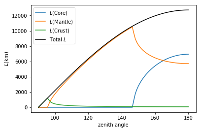
We consider CC and NC interactions separately. CC interactions are straightforward: the neutrino interacts and disappears. NC interactions are more complicated because the neutrino loses a fraction of its energy without disappearing. The average fractional energy loss is 20% at high neutrino energies. The effect of this energy loss can be handled by treating absorption as a two dimensional matrix, relating the energy distribution of neutrinos entering the Earth to the energy distribution of detected neutrinos. This is expressed as a relationship between two fluxes, a function of when the neutrino enters the Earth, and , a function of the detected neutrino energy Aartsen:2017kpd. The result can be expressed in terms of an apparent transparency, , at a single energy , , but, because of energy loss by more energetic neutrinos, this apparent absorption at a given has some dependence on the assumed neutrino spectrum. We avoid this spectral dependence here by considering only monoenergetic neutrinos.
Figure 7 shows as a function of neutrino energy and zenith angle, for and . The shift from shadowing to antishadowing is visible at TeV. The effect of the Earth’s core, with its high iron and likely nickel content, enhances nuclear effects for large zenith angles. These results are shown more quantitatively in Fig. 8 where is presented as a function of for several discrete neutrino energies. drops from about 1.02 to 0.96 for increasing neutrino energies. With trajectories traversing the Earth’s core, the spread is slightly larger due to the greater nuclear effects. The differences between and are shown to be relatively small.


The probability for a neutrino to survive passage through the Earth is
| (28) |
where is the path length through the Earth for a given zenith angle while is the absorption length. Nuclear effects modify the cross section so that where is the cross section for an isoscalar target without shadowing. At an energy and zenith angle where , the change survival probability due to the inclusion of nuclear effects, is roughly comparable to . As rises, so that for long chords through the Earth with a high absorption probability, , small changes in lead to larger changes in the absorption probability.
The larger modification of with due to shadowing could affect the interpretation of anomalous events, such as the possible events observed by ANITA Gorham:2018ydl. For example, ANITA-III event 15717147 traverses a 7,000 km chord through the Earth, corresponding to without nuclear effects, requiring contributions from BSM physics. Reducing the cross section by 4% due to shadowing roughly doubles the survival probability. While this reduction is too small to alter the overall conclusion, a larger reduction in cross section, such as from a colored glass condensate Henley:2005ms might allow this event to be interpreted without requiring BSM physics.
It is important to note that, although we have focused on the best-fit values of EPS09 and EPPS16, the uncertainties are significant. The uncertainties on these values are considerable, more than % and thus larger than . This uncertainty will limit many quantitative analyses.
IV Nuclear effects on inelasticity
The inelasticity of high-energy and charged-current interactions on ice targets has been measured by the IceCube Collaboration Aartsen:2018vez. They separately measured the energy of the hadronic cascade from the struck nucleus, , and the energy of the outgoing muon, , and calculated the inelasticity as . There are two major reconstruction challenges to measuring neutrino inelasticity in a neutrino telescope. First, a muon with energy above 1 TeV travels many kilometers before losing its energy, making the energy determination difficult. Second, there are corrections to account for missing (carried off by the neutrino) and mismeasured (hadronic instead of electromagnetic) energy.
Measurements using starting tracks, defined as a track originating in the active volume of the detector, have many applications. In addition to inelasticity, starting tracks are important for flavor ratio measurements; determining from the difference in inelasticity distributions; and searching for charm production in neutrino interactions Binder:2017rlx. Inelasticity is also relevant for decays since it helps determine the division of energy between the interaction and the , i.e. the energy division between the first and second showers in double-bang ( events with GeV, characterized by a hadronic shower originated when the interacts, a m minimum ionizing track, and a subsequent cascade when the decays) and double-pulse (similar to double-bang but at lower energy, resulting a m minimum ionizing track) events. Changes in the inelasticity distribution may also affect the relationship between and muon energy in through-going muon events.
Ice consists of H2O. As we discuss, hydrogen and oxygen exhibit different nuclear effects. While oxygen is subject to nuclear shadowing, the nuclear effects are dominated by hydrogen because it strongly violates isospin invariance. As Figs. 9 and 10 show, hydrogen has a large , with a rather distinctive energy and inelasticity dependence. The inelasticity can be related to and by
| (29) |
where is the nucleon mass. The inelasticity at a given and fixed is integrated over and . The integral over starts from a minimum of 9 GeV2. The cross sections increase with so that at higher the integral is dominated by .
Figures 9 and 10 show relative to an isospin invariant deuterium target for both protons and H2O, using the CT10 and CT14 CT14 proton PDFs respectively with the EPPS16 nPDFs. Results are given for values of separated by an order of magnitude for from to GeV.
In all cases, as decreases, increases. The shape of for fixed is balance of contributions from and . The range at a given is constrained by the requirement that . For a given , as , can be large, near the maximum of the available range, and will remain less than unity. On the other hand, when , the denominator of Eq. (29) is small so that nust be near its minimum value for to be less than unity.
The choice of proton PDF is important for hydrogen at low inelasticity, where is large and the valence distributions dominate. The top panels of the figures show for hydrogen to deuterium. With a proton target the quark distributions dominate the CC neutrino cross sections while the quark distributions dominate the antineutrino cross sections. In the case of deuterium, the and contributions are balanced. Thus, naively, for neutrinos while, for antineutrinos .
At large , is small and decreases with increasing . Thus, in this range, the sea quark distributions dominate and approaches unity, both as and . In models with a colored glass condensate, or strong nuclear shadowing, the cross section in this region would be reduced.
As , on the other hand, the valence distributions dominate and, here, a difference between the proton PDFs appears at . The change in the slope of in this region is due to the behavior of the valence distribution of the CT10 PDFs. The origin of this rather abrupt change in slope in CT10 is not clear but it is absent in the CT14 sets. We have checked the older proton PDF sets, CTEQ6M and GRV98 GRV98, as well and the calculated values for hydrogen with these sets agree with the CT14 results.

The bottom panels of the figures show for H2O. In this case is dominated by the effect on oxygen. As a consequence of the interplay of and as a function of discussed earlier, the inelasticity curves in these figures trace the inverse of the EPPS16 shadowing ratios in Fig. 2. The rise at low visible for GeV is the result of the high behavior of the shadowing function; the decrease to the minimum of corresponds to the EMC region and the subsequent rise at large is the effect of antishadowing. As increases, the EMC and antishadowing regions become more compressed at low and a decease is seen instead of a rise at larger because is in the shadowing region. Although the effect is relatively independent of whether the interaction is initiated by or , there is a slightly stronger rise for -initiated interactions because of the increased antishadowing in the CC interactions. In addition, as seen in Fig. 4, the distribution dominating antineutrino interactions includes antishadowing on both the valence and sea distributions in this region while the dominant for neutrino interactions shows effects of antishadowing on the valence distribution but shadowing in the same region for the distribution. Finally, we note that the rather large uncertainties visible in both cases for GeV arise here because, even though higher values are probed at large , large uncertainties remain due to the 40 error sets for EPPS16.
The uncertainties on due to the nPDF uncertainties are much larger than for the proton PDFs, on the order of 20%. Because the uncertainties on the nPDFs decrease with , as does the overall nuclear modification, the largest uncertainties are on the smallest values shown for fixed . For fixed , the largest nPDF uncertainties are at small because the smallest range is probed here.
Since the effect on oxygen dominates for H2O, the difference between the CT10 and CT14 PDF sets does not play a significant role here. The relative independence of the nuclear effects on the proton PDFs seen here shows that the choice of proton PDFs did not play a role in the cross section effects discussed in the previous section. Larger nuclear effects, due to color glass condensates or nonlinear parton dynamics, could also alter the inelasticity distribution Goncalves:2013kva. Since and are inversely related, reductions in the cross section are likely to be most prominent at large , corresponding to small .

These nuclear effects have implications for neutrinos and antineutrinos with energies from 100 GeV to a few TeV. At larger energies, the central values of are fairly small but with significant uncertainties due to shadowing.
There are two key points arising from the result that : the nuclear effects are large at small inelasticities and they behave differently for and , particularly for hydrogen. The differences in and may cancel for some effects if there is an equal admixture of and . At TeV, the flux of atmospheric neutrinos (the dominant source) is expected to be in the proportion , rising to 1.75 at 100 TeV Aartsen:2017kpd, resulting in an incomplete cancellation. We will consider the implications of these nuclear effects on a number of different analyses.
IceCube found rather good agreement between their data and inelasticity expectations Aartsen:2017kpd. In their lowest energy bin, TeV, the rise in led to an increase in low inelasticity events. IceCube has limited low inelasticity acceptance in this energy region because of the requirement that the number of detected photons, summed over the IceCube volume, , is large enough to observe the event. The absence of a significant hadronic shower means that most of the neutrino energy is transferred to the muon and escapes the detector. There is room in these data for nuclear effects and efforts have been made to refine the calculations of neutrino scattering rates 2019PhRvD.100i1301G; 2019JHEP…01..217B.
Many other neutrino telescope measurements rely on an implicit knowledge of the inelasticity distribution because many starting-track analyses have an inelasticity-dependent inefficiency. These analyses also require a minimum , or other similar criteria, making them insensitive to events with .
Inelasticity measurements have been used to measure . At energies below about 10 TeV, and have different inelasticity distributions because of the contribution from the valence quarks. At these energies, the flux is dominated by atmospheric which then dominate the measurement. However, with a low-threshold surface air shower detector to veto neutrinos accompanied by an air shower, it might be possible to eliminate most downgoing from the atmosphere. Because and experience different nuclear modifications, measurements of may require a correction for nuclear effects.
In concert with cascades, starting tracks are also used to determine the neutrino flavor ratio. High inelasticity starting tracks will be mistaken for cascades while low inelasticity starting tracks will be missed because of the cut.
Inelasticity also affects the energy that incident transfer to nuclear targets, affecting the energy seen in the first bang of double-bang events.
The excess of low-inelasticity events could be an unexpected background in searches for electromagnetic neutrino interactions which do not involve a nuclear recoil Seckel:1997kk; Beacom:2019pzs and may be relevant in searches for new, BSM interaction topologies.
V Conclusions
We have examined the role of two nuclear effects: shadowing and violation of isospin invariance in ultra-high energy neutrino interactions in both the Earth and in polar ice packs.
Antishadowing decreases the neutrino cross section by about 2% at energies below about 500 TeV while shadowing increases it by about 4% at higher energies. These corrections should be included in new high-accuracy measurements of neutrino absorption in the Earth, including cross section measurements and Earth tomography. These estimated corrections are based on standard QCD evoluion of the nPDFs; new phenomena like the colored glass condensate could perhaps lead to larger modifications.
Nuclear effects in both hydrogen and oxygen affect the inelasticity distribution of neutrino interactions in ice, particularly at low inelasticity, in an energy range that probes quarks at large Bjorken-. The Fermi motion of nucleons in oxygen increases the number of high-momentum quarks and thus the cross section at very low . On the other hand, the difference in sign of the nuclear effects for and on hydrogen will affect measurements of the ratio . These effects are largest for from 100 GeV up to a few TeV. At higher energies, the modifications are shifted to very low and do not contribute greatly.
Although these central shifts are relatively small, the uncertainties are quite significant. Until the uncertainties are reduced, they will limit the precision of many measurements. The uncertainties rise with neutrino energy and are particularly large at the energies targeted by next-generation radio-detection systems Aguilar:2019jay.
With the advent of higher-precision neutrino measurements Robertson:2019wfw, it will be necessary to account for nuclear effects in cross section and tomography measurements. This need will only increase in larger, next-generation neutrino observatories Aartsen:2014njl; Adrian-Martinez:2016fdl; Shoibonov:2019gfj. The introduction of large (order 100 km3) radio-pulse-based neutrino telescopes, with energy thresholds above GeV will also open the door to cross section measurements at higher energies Aguilar:2019jay; Anker:2019mnx, provided that good angular resolution is achieved for near-horizontal events. These experiments may also be able to measure inelasticity in interactions at very high energies by taking advantage of the LPM effect, which elongates electromagnetic showers, allowing them to be separated from the hadronic shower on the basis of Cherenkov cone widths CastroPena:2000fx or via multiple showers Aartsen:2018vez.
Acknowledgements This work was supported in part by the National Science Foundation under grant number PHY-1307472 and the U.S. Department of Energy under contract numbers DE-AC-76SF00098 (S.R.K. and S.A.R.), DE-AC52-07NA27344 and DE-SC-0004014 (R.V).
References
- (1) M. G. Aartsen et al. [IceCube Collaboration], Observation and Characterization of a Cosmic Muon Neutrino Flux from the Northern Hemisphere using six years of IceCube data, Astrophys. J. 833, 3 (2016).
- (2) M. Ackermann et al., Fundamental Physics with High-Energy Cosmic Neutrinos, arXiv:1903.04333 [astro-ph.HE].
- (3) M. G. Aartsen et al. [IceCube Collaboration], A Search for Neutrino Point-Source Populations in 7 Years of IceCube Data with Neutrino-count Statistics, arXiv:1909.08623 [astro-ph.HE].
- (4) M. G. Aartsen et al. [IceCube Collaboration], Flavor Ratio of Astrophysical Neutrinos above 35 TeV in IceCube, Phys. Rev. Lett. 114, 171102 (2015).
- (5) M. G. Aartsen et al. [IceCube Collaboration], Measurement of the Atmospheric Spectrum with IceCube, Phys. Rev. D 91, 122004 (2015).
- (6) M. G. Aartsen et al. [IceCube Collaboration], Measurements using the inelasticity distribution of multi-TeV neutrino interactions in IceCube, Phys. Rev. D 99, 032004 (2019).
- (7) M. G. Aartsen et al. [IceCube Collaboration], Neutrino Interferometry for High-Precision Tests of Lorentz Symmetry with IceCube, Nature Phys. 14, 961 (2018).
- (8) F. Halzen and S. R. Klein, IceCube: An Instrument for Neutrino Astronomy, Rev. Sci. Instrum. 81, 081101 (2010).
- (9) M. G. Aartsen et al. [IceCube Collaboration], The IceCube Neutrino Observatory - Contributions to ICRC 2017 Part II: Properties of the Atmospheric and Astrophysical Neutrino Flux, arXiv:1710.01191 [astro-ph.HE].
- (10) R. Abbasi et al. [IceCube Collaboration], An improved method for measuring muon energy using the truncated mean of , Nucl. Instrum. Meth. A 703, 190 (2013).
- (11) M. G. Aartsen et al. [IceCube Collaboration], Energy Reconstruction Methods in the IceCube Neutrino Telescope, JINST 9, P03009 (2014).
- (12) FASER Collaboration, Detecting and Studying High-Energy Collider Neutrinos with FASER at the LHC, 2019, arXiv:1908.02310, [hep-ex].
- (13) M. G. Aartsen et al. [IceCube Collaboration], Measurement of the multi-TeV neutrino cross section with IceCube using Earth absorption, Nature 551, 596 (2017).
- (14) T. Yuan [IceCube Collaboration], Measurement of the high-energy all-flavor neutrino-nucleon cross section with IceCube, arXiv:1908.07027 [astro-ph.HE].
- (15) M. Bustamante and A. Connolly, Extracting the Energy-Dependent Neutrino-Nucleon Cross Section above 10 TeV Using IceCube Showers, Phys. Rev. Lett. 122, 041101 (2019).
- (16) K. Hoshina, presented at the Neutrino Oscillation Tomography Workshop, Jan. 7-8 2016, Earthquake Research Institute, the University of Tokyo. Slides are available at https://indico.cern.ch/event/442108/contributions/1946171/.
- (17) A. Donini, S. Palomares-Ruiz and J. Salvado, Neutrino tomography of Earth, Nature Phys. 15, 37 (2019).
- (18) J. Ellis, K. Sakurai and M. Spannowsky, Search for Sphalerons: IceCube vs. LHC, JHEP 1605, 085 (2016).
- (19) S. R. Klein, Probing high-energy interactions of atmospheric and astrophysical neutrinos, arXiv:1906.02221 [astro-ph.HE].
- (20) B. L. N. Kenett, On the density distribution within the Earth, Geophys. J. Int. 132, 374 (1998); G. Masters and D. Gubbins, On the resolution of density within the Earth, Phys. Earth and Planetary Interiors, 140, 159 (2003); R. W. L. de Wit, P. J. Kaufl, A. P. Valentine and J. Trampert, Bayesian inversion of free oscillations for Earth’s radial (an)elastic structure, Phys. Earth and Planetary Interiors, 237, 1 (2014).
- (21) A. Cooper-Sarkar, P. Mertsch and S. Sarkar, The high energy neutrino cross-section in the Standard Model and its uncertainty, JHEP 1108, 042 (2011).
- (22) A. Connolly, R. S. Thorne and D. Waters, Calculation of High Energy Neutrino-Nucleon Cross Sections and Uncertainties Using the MSTW Parton Distribution Functions and Implications for Future Experiments, Phys. Rev. D 83, 113009 (2011).
- (23) C. Andreopoulos, C. Barry, S. Dytman, H. Gallagher, T. Golan, R. Hatcher, G. Perdue and J. Yarba, The GENIE Neutrino Monte Carlo Generator: Physics and User Manual, arXiv:1510.05494 [hep-ph]. See also http://www.genie-mc.org/.
- (24) C. Andreopoulos et al., Summary of the NuSTEC Workshop on Shallow- and Deep-Inelastic Scattering, arXiv:1907.13252 [hep-ph].
- (25) F. Gelis, E. Iancu, J. Jalilian-Marian and R. Venugopalan, The Color Glass Condensate, Ann. Rev. Nucl. Part. Sci. 60, 463 (2010).
- (26) E. M. Henley and J. Jalilian-Marian, Ultra-high energy neutrino-nucleon scattering and parton distributions at small , Phys. Rev. D 73, 094004 (2006).
- (27) Y. V. Kovchegov, Introduction to the physics of saturation, AIP Conf. Proc. 1520, 3 (2013).
- (28) V. P. Gonçalves and D. R. Gratieri, High density effects in ultrahigh neutrino interactions, Phys. Rev. D 88, no. 1, 014022 (2013) doi:10.1103/PhysRevD.88.014022 [arXiv:1307.1621 [hep-ph]].
- (29) R. Gauld , Precise predictions for multi-TeV and PeV energy neutrino scattering rates, Phys. Rev. D 100, 9 (2019).
- (30) V Bertone, R Gauld and J Rojo, Neutrino telescopes as QCD microscopes, Journal of High Energy Physics 2019, 1 (2019).
- (31) J. L. Albacete, J. I. Illana and A. Soto-Ontoso, Neutrino-nucleon cross section at ultrahigh energy and its astrophysical implications, Phys. Rev. D 92, no. 1, 014027 (2015) doi:10.1103/PhysRevD.92.014027 [arXiv:1505.06583 [hep-ph]].
- (32) K. J. Eskola, P. Paakkinen, H. Paukkunen and C. A. Salgado, EPPS16: Nuclear parton distributions with LHC data, Eur. Phys. J. C 77, 163 (2017).
- (33) J. Pumplin, D. R. Stump, J. Huston, H. L. Lai, P. M. Nadolsky and W. K. Tung, New generation of parton distributions with uncertainties from global QCD analysis, JHEP 0207, 012 (2002).
- (34) R. Vogt, Shadowing Effects on and Production at Energies Available at the CERN Large Hadron Collider, Phys. Rev. C 92, 281547 (2015).
- (35) C.-Y. Chen, P. S. Bhupal Dev and A. Soni, Standard Model Explanation of the Ultra-high Energy Neutrino Events at IceCube, Phys. Rev. D 89, 033012 (2014).
- (36) A. Baldit et al. [NA51 Collaboration], Study of the isospin symmetry breaking in the light quark sea of the nucleon from the Drell-Yan process, Phys. Lett. B 332, 244 (1994).
- (37) R. S. Towell et al. [NuSea Collaboration], Improved measurement of the anti-d / anti-u asymmetry in the nucleon sea, Phys. Rev. D 64, 052002 (2001).
- (38) K. Nagai [SeaQuest Collaboration], Measurements of Nucleon Structure via Proton-Induced Drell-Yan Process at FNAL SeaQuest, PoS DIS 2018, 033 (2018).
- (39) A. D. Martin, R. G. Roberts and W. J. Stirling, Parton distributions: A Study of the new HERA data, , the gluon and jet production, Phys. Lett. B 387, 419 (1996).
- (40) H. L. Lai, J. Huston, S. Kuhlmann, F. I. Olness, J. F. Owens, D. E. Soper, W. K. Tung and H. Weerts, Improved parton distributions from global analysis of recent deep inelastic scattering and inclusive jet data, Phys. Rev. D 55, 1280 (1997).
- (41) K. J. Eskola, H. Paukkunen and C. A. Salgado, EPS09: A New Generation of NLO and LO Nuclear Parton Distribution Functions, JHEP 0904, 065 (2009).
- (42) M. Tanabashi et al., Review of Particle Physics, Phys. Rev. D 98, 030001 (2018).
- (43) H. L. Lai, M. Guzzi, J. Huston, Z. Li, P. Nadolsky, J. Pumplin, and C.-P. Yuan, New parton distributions for collider physics, Phys. Rev. D 82, 074024 (2010).
- (44) T. Kitagaki et al. [E745 Collaboration], A New Method to Investigate the Nuclear Effect in Leptonic Interactions, Phys. Lett. B 214, 281 (1988).
- (45) V. Emel’yanov, A. Khodinov, S. R. Klein and R. Vogt, The Effect of shadowing on initial conditions, transverse energy and hard probes in ultrarelativistic heavy ion collisions, Phys. Rev. C 61, 044904 (2000).
- (46) J. Gomez et al., Measurement of the -dependence of deep inelastic electron scattering, Phys. Rev. D 49, 4348 (1994).
- (47) P. Amaudruz et al. [New Muon Collaboration], A Reevaluation of the nuclear structure function ratios for D, He, Li-6, C and Ca, Nucl. Phys. B 441, 3 (1995).
- (48) M. Arneodo et al. [New Muon Collaboration], The Structure Function ratios (Li)/(D) and (C)/(D) at small , Nucl. Phys. B 441, 12 (1995).
- (49) M. Arneodo et al. [New Muon Collaboration], The dependence of the nuclear structure function ratios, Nucl. Phys. B 481, 3 (1996).
- (50) J. Ashman et al. [European Muon Collaboration], A Measurement of the ratio of the nucleon structure function in copper and deuterium, Z. Phys. C 57, 211 (1993).
- (51) D. M. Alde et al., Nuclear dependence of dimuon production at 800 GeV. FNAL-772 experiment, Phys. Rev. Lett. 64, 2479 (1990).
- (52) M. A. Vasilev et al. [NuSea Collaboration], Parton energy loss limits and shadowing in Drell-Yan dimuon production, Phys. Rev. Lett. 83, 2304 (1999).
- (53) S. Chatrchyan et al. [CMS Collaboration], Studies of dijet transverse momentum balance and pseudorapidity distributions in pPb collisions at TeV, Eur. Phys. J. C 74, no. 7, 2951 (2014).
- (54) V. Khachatryan et al. [CMS Collaboration], Study of boson production in pPb collisions at 5.02 TeV, Phys. Lett. B 750, 565 (2015).
- (55) V. Khachatryan et al. [CMS Collaboration], Study of boson production in pPb collisions at TeV, Phys. Lett. B 759, 36 (2016).
- (56) G. Aad et al. [ATLAS Collaboration], boson production in Pb collisions at TeV measured with the ATLAS detector, Phys. Rev. C 92, 044915 (2015).
- (57) G. Onengut et al. [CHORUS Collaboration], Measurement of nucleon structure functions in neutrino scattering, Phys. Lett. B 632, 65 (2006).
- (58) S. R. Klein and A. Connolly, Neutrino Absorption in the Earth, Neutrino Cross Sections, and New Physics, arXiv:1304.4891 [astro-ph.HE].
- (59) S. L. Glashow, Resonant Scattering of Antineutrinos, Phys. Rev. 118, 316 (1960).
- (60) F. D. Stacey and P. M. Davis, Physics of the Earth, 4th edition, Cambridge University Press, 2008.
- (61) P. W. Gorham et al. [ANITA Collaboration], Observation of an Unusual Upward-going Cosmic-ray-like Event in the Third Flight of ANITA, Phys. Rev. Lett. 121, 161102 (2018).
- (62) G. A. Binder, Measurements of the Flavor Composition and Inelasticity Distribution of High-Energy Neutrino Interactions in IceCube, UC Berkeley dissertation (2017).
- (63) S. Dulat et al., New parton distribution functions from a global analysis of quantum chromodynamics, Phys. Rev. D 93, 033006 (2016).
- (64) M. Gluck, E. Reya and A. Vogt, Dynamical parton distributions revisited, Eur. Phys. J. C 5, 461 (1998).
- (65) D. Seckel, Neutrino photon reactions in astrophysics and cosmology, Phys. Rev. Lett. 80, 900 (1998).
- (66) B. Zhou and J. F. Beacom, -boson and trident production in TeV–PeV neutrino observatories, arXiv:1910.10720 [hep-ph].
- (67) J. A. Aguilar et al., The Next-Generation Radio Neutrino Observatory – Multi-Messenger Neutrino Astrophysics at Extreme Energies, arXiv:1907.12526 [astro-ph.HE].
- (68) S. Robertson [IceCube Collaboration], Measurement of the multi-TeV neutrino cross section with IceCube using Earth absorption, arXiv:1908.06123 [astro-ph.HE].
- (69) M. G. Aartsen et al. [IceCube Collaboration], IceCube-Gen2: A Vision for the Future of Neutrino Astronomy in Antarctica, arXiv:1412.5106 [astro-ph.HE].
- (70) S. Adrian-Martinez et al. [KM3NeT Collaboration], Letter of intent for KM3NeT 2.0, J. Phys. G 43, 084001 (2016).
- (71) B. Shoibonov [Baikal Collaboration], Baikal-GVD - the Next Generation Neutrino Telescope in Lake Baikal, J. Phys. Conf. Ser. 1263, 012005 (2019). doi:10.1088/1742-6596/1263/1/012005
- (72) A. Anker et al. [ARIANNA Collaboration], Targeting ultra-high energy neutrinos with the ARIANNA experiment, Adv. Space Res. 64, 2595 (2019) doi:10.1016/j.asr.2019.06.016 [arXiv:1903.01609 [astro-ph.IM]].
- (73) J. A. Castro Pena, G. Parente and E. Zas, Measuring the BFKL pomeron in neutrino telescopes, Phys. Lett. B 500, 125 (2001) doi:10.1016/S0370-2693(01)00068-5 [hep-ph/0011043].