Obtaining a Canonical Polygonal Schema from a Greedy Homotopy Basis with Minimal Mesh Refinement
Abstract
Any closed manifold of genus can be cut open to form a topological disk and then mapped to a regular polygon with sides. This construction is called the canonical polygonal schema of the manifold, and is a key ingredient for many applications in graphics and engineering, where a parameterization between two shapes with same topology is often needed. The sides of the gon define on the manifold a system of loops, which all intersect at a single point and are disjoint elsewhere. Computing a shortest system of loops of this kind is NP-hard. A computationally tractable alternative consists in computing a set of shortest loops that are not fully disjoint in polynomial time using the greedy homotopy basis algorithm proposed by Erickson and Whittlesey [1], and then detach them in post processing via mesh refinement. Despite this operation is conceptually simple, known refinement strategies do not scale well for high genus shapes, triggering a mesh growth that may exceed the amount of memory available in modern computers, leading to failures. In this paper we study various local refinement operators to detach cycles in a system of loops, and show that there are important differences between them, both in terms of mesh complexity and preservation of the original surface. We ultimately propose two novel refinement approaches: the former minimizes the number of new elements in the mesh, possibly at the cost of a deviation from the input geometry. The latter allows to trade mesh complexity for geometric accuracy, bounding deviation from the input surface. Both strategies are trivial to implement, and experiments confirm that they allow to realize canonical polygonal schemas even for extremely high genus shapes where previous methods fail.
Index Terms:
Topology, polygonal schema, cut graph, homology, homotopy, cross parameterizationI Introduction
Generating a cross parameterization between two 3D shapes with same genus is an interesting topological problem with practical impact in many fields. Maps of this kind allow to transfer a signal from one shape to the other, and are exploited by many tools in computer graphics, engineering and medicine for various applications, such as texture mapping, remeshing and shape registration, to name a few.
Given two manifolds, a robust way to obtain a cross parameterization consists in cutting both shapes open to topological disks, flatten them on the plane, and then overlap the two disks to obtain a point-to-point correspondence (Figure 2). Computational topology provides a sound theoretical framework to perform each of these operations.
Any closed orientable surface with genus has exactly classes of homotopically independent loops. A system of loops containing one loop from each such class is also a homotopy basis [1]. If cut along its homotopy basis, the surface becomes a topological disk, hence it can be flattened to the plane. In particular, if all loops emanate from a single source and are disjoint elsewhere, cutting the surface yields a polygon with sides, called the canonical polygonal schema of the surface [2] (Figure 1, right). This construction is a topological invariant, hence any two shapes with same genus share the same polygonal schema, which can then be used as a medium to initialize a cross parameterization between them [3, 4, 5]. For this map to be practically useful the cut graph should be shortest, but this latter condition makes the problem NP-hard. A practical alternative consists in computing in polynomial time a shortest system of loops that possibly overlap at some mesh edge, using the greedy homotopy basis algorithm proposed in [1], and then detach such loops in post processing via mesh refinement. Despite apparently trivial, this refinement operation hides some difficulty. In fact, for high genus shapes the system will contain a big number of loops, which will largely snap to the same chains of edges, requiring massive mesh refinement to fully detach them.
To better understand this observation, we recall that the loops of a discrete manifold with genus should all intersect at a unique mesh vertex. For these loops to be fully disjoint, such vertex should have at least incident chains of edges. For example, the Nasty Cheese model shown at the top of Figure 7 has genus 133, which means that the origin of its system of loops should be located at a mesh vertex with at least 532 neighbors. Having a mesh with such a connectivity is practically impossible. In fact, it is known that the average vertex valence for triangle meshes is equal to , which means that already for a manifold with genus 2 the chances that all loops in the basis will be fully disjoint are tiny, and mesh refinement is necessary.
Li and colleagues [3] proposed to use edge splits to detach loops in a greedy homotopy basis. In this paper we show that their refinemet scheme does not scale well on high genus shapes. To make a practical example, the mesh of aforementioned Nasty Cheese originally contained 30K vertices and 60K faces. After refinement it counts 1.5M vertices and 3M faces. Such an incredible growth (roughly 5K times more vertices and triangles) is impractical for applications, and hinders the applicability of this technique for complex shapes. As we show in Section V, for higher genus shapes the refined mesh may become so big that it does not fit the memory of a modern computer, leading to a failure.


In this short paper we analyze alternative refine strategies to detach loops in a given homotopy basis. We first show that, to locally detach two loops, the edge split operator introduces an amount of new elements that depends on the local complexity of the mesh, whereas the vertex split operator has a constant cost of 2 new triangles and 1 new vertex. We also show that, despite topologically optimal, the vertex split may occasionally require deviation from the input mesh. Based on these considerations we propose two alternative refinement strategies: the first one simply substitutes the edge split with the vertex split, obtaining minimal mesh growth; the second one takes also geometry into account, and tries to use as many vertex splits as possible, switching to the costly edge split only when the former would introduce significative deviation from the reference geometry. Users can easily trade mesh size for geometric fidelity by acting on an intuitive parameter that controls when the switch between these operators should occur.
Experiments confirm that our refinement strategies outperform previous refinement techniques for high genus meshes, thus turning this strong theoretical framework into a practical algorithm to robustly initialize cross parameterizations between shapes of any complexity.
II Background and prior works
Before providing a precise formulation of our problem, we briefly introduce basic notions from computational topology and discuss previous works, also fixing the notation.
A manifold is a topological space where each point is locally homeomorphic to . In the discrete setting, manifolds are typically represented as triangle meshes. With abuse of notation, in remainder of the paper we will use the symbol to denote both the manifold and its combinatorial realization. The interpretation will become evident form the context.
Any discrete manifold can be cut through a subset of its edges to form a topological disk. This set of edges is called the cut graph of , and its nodes and arcs define the points and edges of a 2D polygon, called polygonal schema of [7]. The canonical polygonal schema is a mapping of to a regular polygon with sides, where is the genus of . The cut graph associated to such a schema designs on a system of loops that are fully disjoint except at a common vertex, called the origin (or root) of the system. The corners of the gon are the images of the origin, and the edges are images of the loops, which are ordered according to the gluing scheme
with and being two copies of a loop (Figure 1). The canonical polygonal schema has two fundamental properties:
- •
it is a topological invariant, meaning that two manifolds with same genus map to the same polygon (up to a rotational degree of freedom);
- •
it is optimal, in the sense that among all the possible polygonal schemas, the canonical polygon has the least number of edges (i.e. there exists no gon with that is the cut graph of a manifold with genus [8])
Polygonal schemas play a central role in computer graphics, where they are at the basis of numerous applications, such as texture mapping [9], remeshing [10], compression [11], and morphing [12], to name a few. In particular, the properties of the canonical schema make it an appealing starting point to initialize a mapping between two shapes with same genus [3, 4, 5]. In fact, as shown in Figure 2, given two manifolds with genus , and denoting with and their one-to-one maps to the canonical polygon
a cross parameterization can be obtained through the composition
Topologists and pratictioners in computer graphics have widely investigated the problem of computing cut graphs for discrete manifolds. Typically, the goal is to find the cut graph with minimal length, or the one that contains the least number of edges. Erickson and Har-Peled showed that both problems are NP-hard, and proposed a greedy algorithm to compute a approximation of the minimum cut graph in [7]. The so generated cut graphs are not necessarily canonical, hence are not suitable for cross parameterization. Dey and Shipper [8] propose a linear time method to compute a polygonal schema using a breadth-first search on the dual graph. Their cut-graph is not guaranteed to be shortest, and may not yield the canonical schema as well. In [13] Colin de Verdière and Lazarus propose a polynomial time algorithm that inputs a system of loops, and shrinks it in order to find the shortest system of loops in the same homotopy class. To mimic the continuous framework, the authors ”allow the loops to share edges and vertices in the mesh, provided that they can be spread apart on the surface with a thin space so that they become simple and disjoint except at the origin”. The authors do not explain how this operation can be performed, and what impact it has on mesh size. In this paper we focus on this very specific problem, aiming to find the mesh refinement strategy with minimal impact on the input manifold, both in terms of number of discrete elements and geometric fidelity. In [14] and [2] methods to compute system of loops that realize a canonical polygonal schema are presented. As already acknowledged by Lazarus and colleagues in their final remarks ”the obtained loops look too much jaggy and complex to be of any use for practical applications. More work needs to be done in this direction taking into account the geometry of the surface” [14]. To this end, a big step forward was done by Erickson and Whittlesey with their greedy homotopy basis algorithm [1]. At the time of writing, this can be considered to be the state of the art for computing arbitrary polygonal schemas on discrete manifolds. Their method uses the tree-cotree decomposition [15], and is guaranteed to find the shortest system of loops centered at a given mesh vertex in , and – by testing each point in the mesh – the globally shortest system of loops in . It is interesting to notice that while the computation of the shortest cut graph is NP-hard, the shortest system of loops is easy to compute. The difference between these entities relies in how lengths are computed: in a cut graph, each edge in the cut counts once; in a system of loops, each edge counts as many times as the number of loops in the system that traverse it. It follows that the systems of loops computed with the greedy homotopy basis algorithm are practically useful (because they are shortest), but do not allow to realize a canonical schema (because multiple loops snap to the same mesh edges), hence cannot be used to initialize a cross parameterization between two manifolds.
The use of mesh refinement to detach loops in a given homotopy basis is mentioned in a few aforementioned papers but, to the best of our knowledge, only [3] provided an actual algorithm. A similar method was possibly proposed already in [2], but the manuscript misses some technical details, and the algorithm is hardly reproducible. To the best of the author’s knowledge, no alternative refinement schemes have ever been proposed in previous literature.
III Problem Statement and Overview
Given a discrete manifold with genus , our objective is to generate a cut graph that realizes a canonical polygonal schema of , enabling a map to a regular gon. Our algorithm inputs and a system of loops . Loops in are assumed to all emanate from the same origin , but may not be fully disjoint, thus violating the necessary condition to realize a canonical schema, that is
| (1) |
Our method outputs a refined manifold and a new system of loops , such that satisfies Equation 1, and the refinement of is minimal. Without loss of generality, we assume that the input is computed with the greedy homotopy basis algorithm [1]. This is just a practical choice to ensure that loops are shortest. The method works also if loops are not shortest paths, provided that if at some point two loops merge, they follow the same path until they reach the origin .
III-A General Algorithm
To devise a refinement algorithm we start from a basic observation: loops in the system may be partially overlapping, but can never be entirely coincident. This is ensured by the fact that is a system of loops in the sense of [13], hence it is also a cut graph of . If two loops were coincident, would not be a topological disk, thus could not be a cut graph in the first place. It follows that if two loops share a portion of their path towards the origin of the system, there should be a mesh vertex where they begin to coincide. We call this point a merging vertex. Figure 3 (left) shows an example of merging vertex where two loops collapse into a single discrete path that takes to the origin of the system. Note that the number of loops incident to a merging vertex can be much higher (for a manifold with genus the worst case scenario is ). Moreover, each incoming path can be either a single loop or a bundle of multiple loops that already joined at a previous merging vertex. From a computational perspective there is no difference between these cases, single loops or bundles of loops can all be locally disjoint using the same refinement operators.
The main idea of the algorithm is to iteratively push each merging vertex one step forward towards the origin of the system of loops , until all merging points converge to it and Equation 1 is satisfied. In the initialization step, all the merging vertices in are identified and stored in a queue . Then, merging vertices are iteratively extracted and the mesh is locally refined, making sure that all incoming loops traverse the one ring of along a dedicated path. After refinement, the merging point of all such loops has moved to a new mesh vertex which was originally in the one ring of the current . If such a point is not the origin of the system of loops, it is added to the queue. The algorithm stops when is empty. At that point there won’t be any merging vertex in but , thus Equation 1 is satisfied, and a canonical polygonal schema of the refined manifold along the newly generated system can be computed (Figure 1).
Note that the algorithm above does not provide any detail on how the local refinement is performed. There are several options, which produce different results in terms of number of new elements inserted in the mesh, and geometric distance between and . In Section IV we present all the possible alternatives, discussing pros and cons of each strategy.
IV Local Refinement Operators
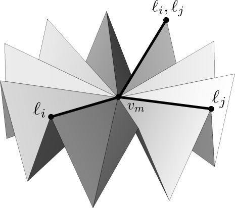
In this section we explore all the alternative ways to split the elements of a simplicial mesh to detach a set of loops around a merging vertex. The basic ingredients for this operation are illustrated in Figure 4. The refinement strategy based on the edge split operator discussed in Section IV-A was already presented in [3]. To the best of our knowledge, the alternatives presented in Section IV-B and IV-D are novel.
The typical configuration is the one shown in Figure 3, where two loops, meet at merging vertex and, from that point on, proceed together towards the origin of the system of loops . Edges traversed by some loop can be locally oriented, such that there is one outgoing edge that points towards the origin of the system, and two (or more) ingoing edges , which all converge to the merging vertex. Rotating from the outgoing edge clock-wise and counter clock-wise towards the first ingoing edges, defines two ordered fans of mesh elements. These are the two alternative domains that can be used to locally refine the mesh, defining two disjoint paths for and within the umbrella of their merging vertex . In the following sub-sections we will detail how each splitting operator can be used to perform such operation.
IV-A Edge Split
Considering a merging vertex and the ordered fan of edges in between an ingoing edge and an outgoing edge , a unique path connecting the associated ingoing vertex and the outgoing vertex can be obtained by splitting all edges in . Denoting with the splitting point of edge , the path is entirely defined within the triangle fan span by , and is also completely disjoint from any other path connecting and . Figure 3 (middle) shows its application to the CCW and CW fans of edges around the merging point . Note that splitting the CCW edge fan introduces 2 new vertices and 4 new triangles, whereas splitting the CW edge fan introduces 1 new vertex and 2 new triangles. In the general case, the mesh grows linearly with the size of the edge fan, and the growth amounts to new vertices, and new triangles. Since there are always two alternative edge fans to be split (CW or CCW), to minimize mesh growth it is preferable to always split the fan with smallest size. Note that the edge split requires that . If the fan of elements in between contains only one triangle and zero edges, loops can be locally split only with the vertex or the triangle split operators.
IV-B Vertex split
Considering the same edge fan around a merging vertex , a unique path connecting and can also be obtained by splitting along the ingoing and outgoing edges that bound . Figure 3 (right) shows an application of this refinement scheme to the CCW and CW fans around the merging point . Note that in both cases the number of new mesh elements amounts to 1 new vertex and 2 new triangles. Differently from the edge split case, this growth is invariant and does not depend on the local complexity of the mesh. Although preferable from a topological point of view, the vertex split operator has a geometric limitation: depending on the geometry of the mesh, the two new triangles incident to the new edge will not adhere to the original mesh, introducing a deviation from the target geometry. An example of failure case is depicted in Figure 5. In general, any time the fan of triangles span by is not planar, the vertex split operator introduces such a deviation.
IV-C Triangle split
Differently form the edge split and the vertex split operator, the triangle split operator can be used to locally detach a pair of loops if and only if the ingoing and the outgoing edges share the same triangle. In that case, adding a new vertex inside the triangle and connecting it to the three corners with new edges generates an alternative path from the ingoing vertex and the outgoing vertex , without passing from the merging vertex (Figure 6). Note that this operation is equivalent to performing a vertex split of along the edges . Also note that if the input system of loops is shortest – as in the case of [1] – this configuration will never occur. If fact, due to the triangular inequality
the path will always be shorter than the path , hence would not be a merging vertex. Considering its limited applicability and the fact that, even when usable, the triangle split is equivalent to the vertex split, this is not a suitable operator to detach loops in a cut graph.
IV-D Hybrid split
The analysis of standard refinement operators revealed that:
- •
the edge split operator can always be used to locally detach loops around a merging vertex without deviating from the input geometry, and introduces an amount of new mesh elements that scales linearly with the number of elements incident to the merging vertex;
- •
the vertex split operator can always be used to locally detach loops around a merging vertex, at the fixed cost of one new vertex and two new triangles. Despite optimal from a topological standpoint, this strategy has a geometric limitation: if none of the two triangle fans are coplanar, the new triangles deviate from the original surface;
- •
the triangle split operator can be used to locally detach loops around a merging vertex if and only if one of the two triangle fans is composed of a single element. When applicable, it is equivalent to the vertex split operator.
We introduce here a fourth option, which aims at combining the positive aspects of the first two operators, using as many vertex splits as possible to minimize mesh growth, and switching to the costly edge split to avoid deviation from the surface. The method is extremely simple, and seamlessly integrates in the global detaching algorithm described in Section III-A.
Given a merging vertex, the hybrid local refinement first checks whether either the CW or CCW fans of elements aside the outgoing edge are roughly planar. If so, it splits the merging vertex along the ingoing and outgoing edges that bound such fan, as described in Section IV-B. If none of the fans are roughly planar, it locally refines the mesh using the edge split operator as described in Section IV-A. To measure planarity we simply consider the maximum angle between the normals of two triangles in the fan of triangles
| (2) |
If the angle above evaluates zero, the fan is planar and the vertex split operator can be used without introducing any deviation from the input surface. In all other cases some deviation from the reference geometry will occur. Assuming the mesh is planar and the vertex split operator is used, positioning the new vertex in the one ring of the merging vertex is also critical to ensure that no triangle will flip its orientation in the refined mesh. Making sure that stays inside the polygon defined by the boundaries of the edge fan is not enough, because such polygon may be non convex ( and may form a concave angle). We practically solve this issue by initializing the new point as
where is initially set to 0.75, and is the vertex opposite to along the edge , which is median in the edge fan being split. If any of the triangles incident to is flipped, we halve and update its position, until a valid position is found. Such a position always exists if do not coincide. In practice we use the vertex split operator even when the fan of elements is roughly planar. To do so we simply test Equation 2 with a threshold angle set by the user. For more details on the actual values refer to Section V.

| Edge Split | Vert Split | Hybrid Split | ||||||||||||
| Model | #V/#T | genus | #V/#T | % | Val. | #V/#T | % | Val. | #V/#T | % | Val. | Cop. | V/E % | H |
| Bamboo Basket | 8K/16K | 163 | out of memory (>16GB) | 26K/53K | 237% | 114/17.6 | 337K/675K | 4229% | 43/14.3 | 64%/36% | ||||
| Buckyball | 5K/11K | 31 | 16K/32K | 202% | 22/9.5 | 7K/14K | 35% | 16/8.5 | 13K/26K | 145% | 22/9.1 | 40%/60% | ||
| Chair | 47K/94K | 245 | out of memory (>16GB) | 98K/197K | 109% | 207/28.4 | 2.7M/5.4M | 5772% | 156/24.9 | 70%/30% | ||||
| Eight | 0.75K/1.5K | 2 | 0.78K/1.5K | 2% | 9/6.9 | 0.75/1.5K | 1% | 9/6.9 | 0.78K/1.5K | 1% | 9/6.9 | 22%/78% | ||
| Fertility | 6K/12K | 4 | 6K/12K | 4% | 11/9.2 | 6K/12K | 2% | 11/8 | 6K/12K | 4% | 11/9.1 | 11%/89% | ||
| Hexbowl | 34K/70K | 260 | out of memory(>16GB) | 110K/220K | 219% | 163/13.1 | 875K/1.7M | 2450% | 164/12.7 | 60%/40% | ||||
| Nasty Cheese | 30K/61K | 133 | 1.5M/3M | 4902% | 49/11.1 | 48K/97K | 60% | 93/11.5 | 177K/355K | 490% | 62/11.8 | 63%/37% | ||
| Polycube | 1K/2K | 50 | 47K/93K | 57016% | 39/8.2 | 10K/21K | 1189% | 29/7.9 | 10K/21K | 1197% | 182/28.1 | 99%/1% | ||
| Radiator | 33K/68K | 204 | out of memory(>16GB) | 65K/130K | 92% | 578/123.9 | 2.1M/4.2M | 6155% | 316/78.3 | 81%/19% | ||||
| Thingi 1764652 | 4.2K/9K | 117 | 32K/65K | 7627% | 32/15.1 | 11K/22K | 153% | 45/13.1 | 54K/109K | 1179% | 43/14.8 | 60%/40% | ||
V Results and Discussion
In this section we analyze the performances of the refinement strategies previously presented. Since we are mostly interested in the scalability of these operators, we focused our analysis on high genus meshes, which we mostly gathered from the Thingi10K [16] dataset. For completeness, a few meshes with lower genus have also been considered (e.g. Eight, Fertility). Our experimental setup is as follows: for each model we first compute a generic system of loops with [1]. To reduce the computational effort, rather than computing the globally shortest system of loops we randomly pick a mesh vertex and compute the shortest system centered at it. We then apply the three refinement algorithms to detach all loops except at their basis, producing three alternative cut graphs that admit a canonical polygonal schema (Figure 7).
In Table I we report numerical results. For each refinement strategy we report mesh size before and after refinement, and the growth rate, measured in percentage w.r.t. the initial number of vertices. Since for the edge split and the hybrid strategies the number of elements incident to a merging vertex is deeply connected with the amount of new elements introduced in the mesh, we also report minimum and average valence of the merging vertices processed during refinement. Note that the maximum valence reported is always lower than (with being the genus), which is the valence of the vertex at which the system of loops is centered. For the hybrid scheme, we also report the amount of vertex and edge splits executed, the coplanarity threshold we used to choose between them, as well as the maximum and average Hausdorff distances from the input manifold, computed with Metro [17].
Looking at numbers, it becomes very clear that for low genus meshes there is no significant difference between the three refinement operators we presented. This is not surprising, in fact low genus manifolds require a small amount of splits, which do not impact mesh size whatever strategy is used. For meshes with growing genus the weaknesses of the edge split operator become evident, and manifolds grow up to several orders of magnitude with respect to their original size. In four cases our reference implementation was not even able to complete the refinement, as the mesh was bigger than the memory at disposal in our testing hardware (16GB of RAM). Conversely, the vertex split operator always provides minimal mesh refinement, exhibiting a mesh growth that is always lower than 250% except for one mesh. The hybrid refinement stays in between, and the amount of mesh growth it produces closely relates with the geometry of the manifold. For largely planar meshes like the polycube, its performances are almost equivalent to the vertex split operator (only 1% of edge splits performed), whereas for smooth geometries the amount of edge splits may grow up to 89% (for Fertility, the worst result in this regard). Note that these numbers depend from the coplanarity threshold of choice. Smaller angles would increase the amount of edge splits, whereas larger angles would reduce it, possibly at the cost of a bigger deviation from the input geometry. We empirically observed that a threshold of 5 degrees provides a good tradeoff between the amount of vertex splits executed and the deviation from the input mesh. With this value the average Hausdorff distance was always below 4e-5. Users can intuitively play with this parameter, trading mesh size for geometric accuracy.
Taking a closer look at why the disparity between the edge split and the vertex split is so big, one plausible explanation is that the edge split introduces, for each merging vertex processed, an amount of new mesh elements that scales linearly with the size of the triangle fan being split (Section IV-A). To this end, it should be noted that even though the average vertex valence for a triangle mesh is 6, the connectivity generated by these refinement operators produces vertices with bigger valence, especially for high genus meshes where multiple loops snap to the same path. To make an example, if at a merging vertex there are three incoming edges, each one carrying 10 loops, after detachment the outgoing vertex adjacent to it will have valence 32 (30 plus 2 incident edges in the original one ring the merging vertex). To fully detach all loops, one similar vertex will be produced as many times as the number of discrete steps between the initial position of the merging vertex and the root of the system of loops. Conversely, the vertex split operator only adds two new triangles and one new vertex for each loop being detached, and is therefore not affected by the valence of the merging vertices, which is in average higher for this scheme (Table I).
In Figure 8 we study the growth rate of the three splitting operators on a sequence of meshes with increasing genus. For this experiment, we considered as base mesh a genus one polycube like the one showed in Figure 2, and produced a sequence of polycubes concatenating multiple occurrences of it. Overall, we produced 50 meshes with genus going from 1 to 50. As shown in the plot, the edge split operator has the worst performances, exhibiting a super quadratic growth in the number of vertices. After detaching all the loops in the system, the mesh of the torus with genus 50 contains more vertices than its original version. Conversely, the vertex split operator exhibits a linear growth in mesh size, having a maximal growth in the number of vertices equal to . Interestingly, also the hybrid scheme has the same asymptotic behaviour, and has a maximal growth in the number of vertices equal to . As already pointed out before, note that the performances of the hybrid scheme depend from both topology and geometry, and may therefore be different for manifolds with different embedding. Nevertheless, polycubes are an interesting case of study because of their practical relevance: maps between a shape and a polycube abstraction of it are at the base of many applications, such as texturing, hexmeshing and spline fitting [6, 3].
VI Conclusions and future works
We showed that detaching cycles in a system of loops using the edge split operator triggers a mesh growth that explodes with genus, producing overly big meshes with little practical usefulness. In alternative we propose two novel refinement operators. The first one is based on the vertex split, and outperforms methods based on the edge split by introducing a minimal amount of elements in the mesh. Despite optimal from a topological point of view, this scheme may introduce deviation from the input surface. The second alternative addresses this limitation, and proposes to use as many vertex splits as possible, switching to the costly edge split only when significative surface deviation occurs. An intuitive parameter that measures the local planarity of the mesh allows users to trade between mesh size and geometric fidelity. In the technical part we also describe two simple heuristics to evaluate local planarity and to robustly position new mesh vertices. Although these methods worked fine in all our experiments, depending on the needs they could be easily substituted with more accurate (or faster) alternatives.
We support our claims with a variety of results, obtained on discrete manifolds that span from low to very high genus, and from smooth to CAD-like shapes. The proposed algorithms are based on well established local operators for simplicial meshes. These operators are already implemented in many geometry processing toolkits, making our results easy to reproduce. Nevertheless, we release a reference implementation of all the splitting methods presented in this paper (included the basic edge split strategy) inside Cinolib [18].
Despite conceptually simple, we believe that this work makes one step forward towards the robust and computationally affordable generation of cross maps between complex shapes. Interesting results have already been presented for disk-like topologies [19], and we expect more and more papers to come in future years. In the same spirit of recent works for the robust computation of planar maps, which start with Tutte’s embedding and then cure distortion [20, 21, 22], we foresee a similar pipeline for cross maps between shapes, where manifolds are first cross mapped via their canonical schema, and then the polygon is evolved to minimize distortion. Note that this problem is much harder: partly because distortion minimization should consider the composition of two maps that overlap to one another, but more importantly because there are alternative ways to overlap two gons (i.e., which handle maps to which?), which makes it a problem with mixed discrete and continuous degrees of freedom for which, to the best of our knowledge, no effective solution is available in literature. Finally, we also plan to study the suitability of our cut graphs as an alternative to the ones described in [23] for the computation of global seamless parameterizations.
References
- [1] J. Erickson and K. Whittlesey, “Greedy optimal homotopy and homology generators,” in Proceedings of the sixteenth annual ACM-SIAM symposium on Discrete algorithms. Society for Industrial and Applied Mathematics, 2005, pp. 1038–1046.
- [2] G. Vegter and C. K. Yap, “Computational complexity of combinatorial surfaces,” in Proceedings of the sixth annual symposium on Computational geometry. ACM, 1990, pp. 102–111.
- [3] X. Li, Y. Bao, X. Guo, M. Jin, X. Gu, and H. Qin, “Globally optimal surface mapping for surfaces with arbitrary topology,” IEEE Transactions on Visualization and Computer Graphics, vol. 14, no. 4, pp. 805–819, 2008.
- [4] C. Carner, M. Jin, X. Gu, and H. Qin, “Topology-driven surface mappings with robust feature alignment.” in IEEE Visualization, vol. 2005, 2005, pp. 543–550.
- [5] H. Wang, Y. He, X. Li, X. Gu, and H. Qin, “Polycube splines,” in Proceedings of the 2007 ACM symposium on Solid and physical modeling. ACM, 2007, pp. 241–251.
- [6] M. Livesu, N. Vining, A. Sheffer, J. Gregson, and R. Scateni, “Polycut: Monotone graph-cuts for polycube base-complex construction,” ACM Transactions on Graphics (Proc. SIGGRAPH ASIA 2013), vol. 32, no. 6, 2013.
- [7] J. Erickson and S. Har-Peled, “Optimally cutting a surface into a disk,” Discrete & Computational Geometry, vol. 31, no. 1, pp. 37–59, 2004.
- [8] T. K. Dey and H. Schipper, “A new technique to compute polygonal schema for 2-manifolds with application to null-homotopy detection,” Discrete & Computational Geometry, vol. 14, no. 1, pp. 93–110, 1995.
- [9] A. Sheffer, B. Lévy, M. Mogilnitsky, and A. Bogomyakov, “Abf++: fast and robust angle based flattening,” ACM Transactions on Graphics (TOG), vol. 24, no. 2, pp. 311–330, 2005.
- [10] P. Alliez, M. Meyer, and M. Desbrun, “Interactive geometry remeshing,” in ACM Transactions on Graphics (TOG), vol. 21, no. 3. ACM, 2002, pp. 347–354.
- [11] G. Taubin and J. Rossignac, “Geometric compression through topological surgery,” ACM Transactions on Graphics (TOG), vol. 17, no. 2, pp. 84–115, 1998.
- [12] V. Kraevoy and A. Sheffer, “Cross-parameterization and compatible remeshing of 3d models,” ACM Transactions on Graphics (TOG), vol. 23, no. 3, pp. 861–869, 2004.
- [13] É. C. De Verdière and F. Lazarus, “Optimal system of loops on an orientable surface,” Discrete & Computational Geometry, vol. 33, no. 3, pp. 507–534, 2005.
- [14] F. Lazarus, M. Pocchiola, G. Vegter, and A. Verroust, “Computing a canonical polygonal schema of an orientable triangulated surface,” in Proceedings of the seventeenth annual symposium on Computational geometry. ACM, 2001, pp. 80–89.
- [15] D. Eppstein, “Dynamic generators of topologically embedded graphs,” in Proceedings of the fourteenth annual ACM-SIAM symposium on Discrete algorithms. Society for Industrial and Applied Mathematics, 2003, pp. 599–608.
- [16] Q. Zhou and A. Jacobson, “Thingi10k: A dataset of 10,000 3d-printing models,” arXiv preprint arXiv:1605.04797, 2016.
- [17] P. Cignoni, C. Rocchini, and R. Scopigno, “Metro: measuring error on simplified surfaces,” in Computer Graphics Forum, vol. 17, no. 2. Wiley Online Library, 1998, pp. 167–174.
- [18] M. Livesu, “cinolib: a generic programming header only c++ library for processing polygonal and polyhedral meshes,” Transactions on Computational Science XXXIV, 2019, https://github.com/mlivesu/cinolib/.
- [19] P. Schmidt, J. Born, M. Campen, and L. Kobbelt, “Distortion-minimizing injective maps between surfaces,” ACM Transactions on Graphics (TOG), vol. 38, no. 6, pp. 1–15, 2019.
- [20] M. Rabinovich, R. Poranne, D. Panozzo, and O. Sorkine-Hornung, “Scalable locally injective mappings,” ACM Transactions on Graphics (TOG), vol. 36, no. 4, p. 37a, 2017.
- [21] J. Smith and S. Schaefer, “Bijective parameterization with free boundaries,” ACM Transactions on Graphics (TOG), vol. 34, no. 4, p. 70, 2015.
- [22] L. Liu, C. Ye, R. Ni, and X.-M. Fu, “Progressive parameterizations,” ACM Transactions on Graphics (TOG), vol. 37, no. 4, p. 41, 2018.
- [23] M. Campen, H. Shen, J. Zhou, and D. Zorin, “Seamless parametrization with arbitrary cones for arbitrary genus,” ACM Transactions on Graphics (TOG), vol. 39, no. 1, pp. 1–19, 2019.