Forecasting multiple functional time series in a group structure: an application to mortality

Let $y_{t}^{(j)}(x_{i})$ be the log central mortality rates observed at the beginning of each year $t=1,2,\dots,n$ at observed ages $(x_{1},x_{2},\dots,x_{p})$ where $x$ is a continuous age variable, $p$ denotes the number of ages, and superscript ^(j) represents $j$^th series. By applying a penalized regression spline smoothing, we obtain smoothed series, $f_{t}^{(j)}(x)$ that is observed at discrete data points with errors.

As in the case of multiple subpopulations, the multivariate functional time series are combined in a vector with

These multivariate functions are defined over the same domain $\Gamma$. The common domain $\Gamma$ must be compact sets in $R^{\omega}$, $\omega\in N$ with finite measure and with each element $f^{(j)}(x)$ assumed to be a square-integrable function $\mathcal{L}^{2}(\Gamma)$, where $j=1,\dots,\omega$. For mathematical convenience, we let

where $\bm{0}$ denotes a vector of zeros. For $x,z\in\Gamma$, the cross-covariance function is defined with elements

From the cross-covariance function, we can deduce the eigenfunction as

where $\mathcal{K}$ induces the kernel of an integral operator, $\phi\mapsto\mathcal{K}\phi$ is a square-integrable function.

From the cross-covariance function, there exists an orthonormal sequence $(\phi_{k})$ of continuous functions in $\mathcal{L}^{2}(\Gamma)$ and a non-increasing sequence, $\lambda_{k}$, of positive numbers, such that

By functional principal component analysis, a de-centered stochastic process $f_{t}^{(j)}(x)$ can be expressed as

where $\big\{\phi_{1}^{(j)}(x),\dots,\phi_{K}^{(j)}(x)\big\}$ is a set of the first $K$ functional principal components for the $j$^th subpopulation; $\bm{\beta}_{1}^{(j)}=\big(\beta_{1,1}^{(j)},\dots,\beta_{n,1}^{(j)}\big)^{\top}$ and $\big\{\bm{\beta}^{(j)}_{1},\dots,\bm{\beta}^{(j)}_{K}\big\}$ denotes a set of principal component scores and $\bm{\beta}_{k}^{(j)}\sim N\big(0,\lambda_{k}^{(j)}\big)$ where $\lambda_{k}^{(j)}$ is the $k^{\text{th}}$ eigenvalue of the covariance function for the $j^{\text{th}}$ subpopulation in (3); and $K<n$ is the retained number of functional principal components. Expansion (6) facilitates dimension reduction as the first $K$ terms often provide a good approximation to the infinite sum, and thus the information contained in $\bm{f}^{(j)}(x)=[f^{(j)}_{1}(x),\dots,f^{(j)}_{n}(x)]$ can be adequately summarized by the $K$-dimensional vector $\big(\bm{\beta}^{(j)}_{1},\dots,\bm{\beta}^{(j)}_{K}\big)$.

The optimal value of $K$ can be selected by a ratio method:

or the optimal value of $K$ can be selected by explaining at least 90% of total variation:

We take the maximum of the $K$ values obtained from (7) and (8).

The matrix formulation of (6) is

where $\bm{f}_{t}(x)=\left[f_{t}^{(1)}(x),f_{t}^{(2)}(x),\dots,f_{t}^{(\omega)}(x)\right]$, $\bm{\beta}_{t}=\left[\beta_{t,1}^{(1)},\dots,\beta_{t,K}^{(1)},\beta_{t,1}^{(2)},\dots,\beta_{t,K}^{(2)},\dots,\beta_{t,1}^{(\omega)},\dots,\beta_{t,K}^{(\omega)}\right]$ being the vector of the basis expansion coefficients, and

where $\ell=\omega\times K$.

The advantage of our multivariate functional time-series forecasting method is that the correlations among sub-populations can be captured in the cross-covariance structure described in (3). The disadvantage of our proposal is that we implicitly assume that all series share the same retained number of functional principal components, and consequently we may lose forecast accuracy for a particular series.

Based on the estimated covariance function, we can extract empirical functional principal component functions $\bm{\mathcal{B}}=\{\widehat{\phi}^{(j)}_{1}(x),\dots,\widehat{\phi}^{(j)}_{K}(x)\}$ using functional principal component analysis. Conditioning on the smoothed functions $\bm{f}^{(j)}(x)=\{f_{1}^{(j)}(x),\dots,f_{n}^{(j)}(x)\}$ and the estimated functional principal components $\bm{\mathcal{B}}$, the $h$-step-ahead point forecast of $f_{n+h}^{(j)}(x)$ can be obtained as

where $\widehat{\beta}_{n+h|n,k}^{(j)}$ represents the time-series forecasts of the $k$^th principal component scores for the $j$^th subpopulation, which can be obtained by using autoregressive integrated moving average models.

We introduce the grouped forecasting methods using the Japanese age-specific mortality rates provided in Section 2. The Japanese data follow a three-level geographic group structure, coupled with a sex-grouping variable (Shang and Haberman 2017). The geographical group structure is presented in Figure 1. Japan can be split into eight regions from north to south, which is then divided into 47 prefectures (Shang and Haberman 2017).

The data can also be split by sex. Each of the nodes in the geographical group structure can also be split into males and females. We refer to a particular disaggregated series using the notation $X\ast S$, referring to the geographic area $X$ and the sex $S$, where $X$ can take the values shown in Figure 1 and $S$ can take values M (males), F (females) or T (total). For example, R1$\ast$ F denotes females in Region 1; P1$\ast$ T denotes all females and males in Prefecture 1; Japan $\ast$ M denotes all males in Japan.

Denote E${}_{X\ast S,t}(x)$ as the exposure-to-risk for series $X\ast S$ in year $t$ and age $x$, and let $\text{D}_{X\ast S,t}(x)$ be the number of deaths for series $X\ast S$ in year $t$ and age $x$. The age-specific mortality rate is $\text{R}_{X\ast S,t}(x)=\text{D}_{X\ast S,t}(x)/\text{E}_{X\ast S,t}(x)$.

To simplify expressions, we will drop the age argument $(x)$. Then for a given age, we can write

or $\bm{R}_{t}=\bm{S}_{t}\bm{b}_{t}$, where $\bm{R}_{t}$ is a vector containing all series at all levels of disaggregation, $\bm{b}_{t}$ is a vector of the most disaggregated series, and $\bm{S}_{t}$ shows how the two are connected.

As the simplest grouped forecasting method, the bottom-up method first generates independent forecasts for each series at the most disaggregated level, and then aggregates these to produce all of the required forecasts (Shang and Haberman 2017). For example, reverting to the Japanese data, we first generate $h$-step-ahead independent forecasts for the most disaggregated series, namely $\widehat{b}_{n+h}=\big[\widehat{R}_{\text{P1}\ast\text{F},n+h},\widehat{R}_{\text{P1}\ast\text{M},n+h},\dots,$ $\widehat{R}_{\text{P47}\ast\text{F},n+h},\widehat{R}_{\text{P47}\ast\text{M},n+h}\big]^{\top}$. Then, we obtain forecasts for all series as

where $\overline{\bm{R}}_{n+h}^{\text{BU}}$ denotes the reconciled forecasts obtained from the bottom-up method.

The bottom-up method performs well when the bottom-level series have a high signal-to-noise ratio. In contrast, the bottom-up method may lead to inaccurate forecasts of the top-level series, in particular when there are missing or noisy data at the bottom level (Shang and Haberman 2017; Shang and Hyndman 2017, see, e.g.,).

Instead of considering only the bottom-level series, Hyndman et al. 2011 have proposed the optimal-combination method where independent forecasts for all series are computed independently, and then the resultant forecasts are reconciled so that they satisfy the aggregation constraints via the summing matrix. The optimal-combination method combines the independent forecasts through linear regression by generating a set of revised forecasts that are as close as possible to the independent forecasts, but that also aggregate consistently within the group. The method is derived by expressing the independent forecasts as the response variable of the linear regression

where $\widehat{\bm{R}}_{n+h}$ is a matrix of $h$-step-ahead independent forecasts for all series, stacked in the same order as for the original data; $\bm{\beta}_{n+h}=\mathbb{E}[\bm{b}_{n+h}|\bm{R}_{1},\dots,\bm{R}_{n}]$ is the unknown mean of the independent forecasts of the most disaggregated series; and $\bm{\epsilon}_{n+h}$ represents the reconciliation errors.

To estimate the regression coefficient, Hyndman et al. 2011 have proposed an ordinary least-squares solution,

The revised forecasts are given by

Forecast combination involves the computation of weighted means for the forecast. The averaged forecast for horizon $h$ is computed as the weighted mean:

where $\overline{\bm{R}}_{n+h}^{g}$ denotes forecasts obtained from a grouped forecasting method, such as the bottom-up or optimal-combination method, and $\overline{\bm{R}}_{n+h}^{\text{comb}}$ represents the model-averaged forecast; and $(w_{1},w_{2},\dots,w_{G})$ are weights that sum to 1.

The crux of the problem lies in the selection of weights. Recent studies found that past performance information enables the use of unequal weighting combinations, but simple combination methods have been shown to be robust in many settings. Here, we consider two heuristics for combining the midpoint (i.e., point forecast) and endpoints (i.e., interval forecasts) (see Gaba et al. 2017, for other heuristics). First, we combine point and interval forecasts obtained from two grouped forecasting methods with equal weighting. Second, we consider an envelope of prediction intervals and simple averaging of midpoints.

Average (Av). From the viewpoint of combining interval forecasts, $\overline{\bm{R}}_{n+h,L}^{\text{comb, Av}}=\frac{1}{G}\sum^{G}_{g=1}\overline{\bm{R}}_{n+h,L}^{g}$ and $\overline{\bm{R}}_{n+h,U}^{\text{comb, Av}}=\frac{1}{G}\sum^{G}_{g=1}\overline{\bm{R}}_{n+h,U}^{g}$, where $[\overline{\bm{R}}_{n+h,L}^{g},\overline{\bm{R}}_{n+h,U}^{g}]$ for $g=1,\dots,G$ denote the lower and upper bounds for a random variable $\overline{\bm{R}}_{n+h}$, and $G$ denotes the number of grouped forecasting methods. This heuristic takes a simple average of the midpoint and endpoints. For combining point and interval forecasts, simple averages are often considered as the benchmark because of their simplicity, good performance, and robustness. When the lower and upper bounds are symmetric, Av combination method corresponds to averaging quantiles, which bridges the gap between interval forecast combination and quantile averaging (Gaba et al. 2017, see, e.g,).

Envelope (En) of endpoints and simple averaging of midpoints. The individual method tends to be overconfident, so an envelope method combines the prediction intervals by taking an extreme viewpoint. The combined $\big(\overline{\bm{R}}_{n+h,L}^{\text{comb, En}},\overline{\bm{R}}_{n+h,U}^{\text{comb, En}}\big)$ are obtained by $\overline{\bm{R}}_{n+h,L}^{\text{comb, En}}=\min(\overline{\bm{R}}_{n+h,L}^{1},\dots,\overline{\bm{R}}_{n+h,L}^{G})$ and $\overline{\bm{R}}_{n+h,U}^{\text{comb, En}}=\max(\overline{\bm{R}}_{n+h,U}^{1},\dots,\overline{\bm{R}}_{n+h,U}^{G})$. This heuristic is conservative but can overcome the overconfident issue, as each method only presents a partial view of reality. The simple average of the lower and upper bounds obtained from $G$ number of methods provides a combined point forecast, where

$$\overline{\bm{R}}_{n+h}^{\text{comb, AvInt}}=\frac{1}{G}\sum^{G}_{g=1}\frac{\overline{\bm{R}}_{n+h,L}^{g}+\overline{\bm{R}}_{n+h,U}^{g}}{2}.$$

(17)

Since the bottom-level forecasts are mortality rates, we ought to take into account forecast exposure-to-risk in order to reconcile death counts with respect to the group structure. The observed ratios that form the $S_{t}$ summing matrix are forecast using the automatic ARIMA algorithm of Hyndman and Khandakar 2008, when age $x=60$. For age above 60, we assume the exposure-to-risk of age $x+1$ in year $t+1$ will be the same as the exposure-to-risk of age $x$ in year $t$ (Shang and Haberman 2017, see also). For example, let $p_{t}=\text{E}_{\text{P1}\ast\text{F},t}/\text{E}_{\text{Japan}\ast\text{T},t}$ be a non-zero element of $S_{t}$. Given that we have observed $\{p_{1},\dots,p_{n}\}$, an $h$-step-ahead forecast $\widehat{p}_{n+h}$ can be obtained. The forecasts of ratios between any two exposure-to-risks are used to form the matrix $\bm{S}_{n+h}$. To ensure summability to 1 in each row of the group structure, every non-zero ratio is normalized by dividing the sum of ratios in each row.

The potential improvement in forecast accuracy of the reconciliation methods partially relies on the accurate forecast of the $S$ matrix. Recall that the $S$ matrix includes ratios of forecast exposure-at-risk. Our cohort assumption is reasonable because it allows us to forecast ratios and populate the $S$ matrix. Shang and Haberman 2017 and Shang and Hyndman 2017 compare point forecast and interval forecast accuracies between the reconciliation methods, with the forecast $S$ matrix and actual holdout $S$ matrix, and found that it is advantageous to use the forecast $S$ matrix.

For the national and sub-national mortality rates, we examine the goodness-of-fit of the proposed multivariate functional time-series method to the observed data. Because the mortality rates for subpopulations may have different mean and variance terms, we standardized age-specific mortality rates by subtracting the mean function and dividing the standard deviation function before implementing a functional principal component analysis to a stacked data matrix of size $n\times(p\times\omega)$. For the Hokkaido data, the selected number of components is one (this is effectively a Lee-Carter type model).

In the first column of Figure 2, we present the mean functions of the female and male smoothed log mortality rates. In the second and third columns, we present the first functional principal component, which accounts for around 88% of the total variation in the joint female and male sub-populations. Given that the principal component scores are surrogates for the original functional time series, they are forecast to continue to decrease over the next 20 years. We note that the first functional principal component models the female and male mortality data at younger and older ages.

We measure goodness-of-fit via a functional version of the $R^{2}$ criterion. It is given as

where $y_{t}^{(j)}(x)$ denotes the observed age-specific log mortality rates at each $t$ for the $j$^th subpopulation, $\widehat{f}_{t}^{(j)}(x)$ denotes the fitted age-specific log mortality rates. The larger the $R^{2}$ value is, the better is the goodness-of-fit by a model. It is possible for the $R^{2}$ criterion to take negative values. A negative $R^{2}$ value implies that the fitted model may not well explain the raw data that are likely to contain a large amount of measurement errors. From a negative $R^{2}$ value, we can quantify the amount of measurement errors exhibited in a data set and the degree of smoothing that the raw mortality data require.

In Table 2, we report the goodness-of-fit of the univariate and multivariate functional time-series methods, as measured by the $R^{2}$ criterion defined in (18). For both female and male series, the multivariate functional time-series method generally achieves a better goodness-of-fit result than the univariate functional time-series method. The superiority of the multivariate functional time series method is because it can incorporate correlation between multiple series. This correlation provides additional information that is not possessed by the univariate functional time series method.

Based on the observed mortality rates from 1975 to 2016, we produce the 20-years-ahead point forecasts of female and male age-specific mortality rates from 2017 to 2036. As shown in Figure 3 for the case of Hokkaido, the age-specific mortality rates are continuing to decline, and the forecast female mortality rates are likely to be lower than the male mortality rates.

Using the first 27 observations from 1975 to 2001 in the Japanese age-specific mortality rates, we produce one- to 15-step-ahead point forecasts. Through an expanding window approach, we re-estimate the parameters in the time series forecasting models using the first 28 observations from 1975 to 2002. Point forecasts from the estimated models are then produced for one- to 14-step-ahead. We repeat this process by increasing the sample size by one year until reaching the end of the data period in 2016. This process produces 15 one-step-ahead forecasts, 14 two-step-ahead forecasts, $\dots$, and one 15-step-ahead forecast. By comparing these forecasts with the holdout samples, we evaluate the out-of-sample point forecast bias and accuracy.

To assess the point forecast bias, we consider the mean forecast error (MFE). For each series $j$, MFE can be written as

where $h$ denotes forecast horizon, $y_{n+\xi}^{(j)}(x_{i})$ denotes the actual holdout sample for the $i$^th age and $\xi$^th curve in the $j$^th series, while $\widehat{y}_{n+\xi}^{(j)}(x_{i})$ denotes the point forecasts for the holdout sample. To assess the point forecast accuracy, we use the mean absolute forecast error (MAFE) defined as

Since the number of series is different across different levels of disaggregation, we obtain an overall assessment of point forecast bias and accuracy by taking the simple average of the error measures across the number of series at each level. With 15 different forecast horizons, we consider the mean and median values to evaluate overall point forecast bias and accuracy between the two functional time-series methods for national and sub-national mortality forecasts.

Averaging over all the series at each level of the group structure, Figure 4 compares MFE$(h)$ between the univariate and multivariate functional time-series methods. As measured by the MFE, the multivariate functional time-series method generally produces more accurate point forecast bias than the ones obtained using the univariate functional time-series method. Using the multivariate functional time-series method, the smallest bias can be achieved by using the forecast combination method with simple averaging of midpoints at each level of the group structure. The superior forecast accuracy of the multivariate functional time-series method over the univariate functional time-series method stems from two sources:

The advantage of this forecast combination is that it can reduce bias.

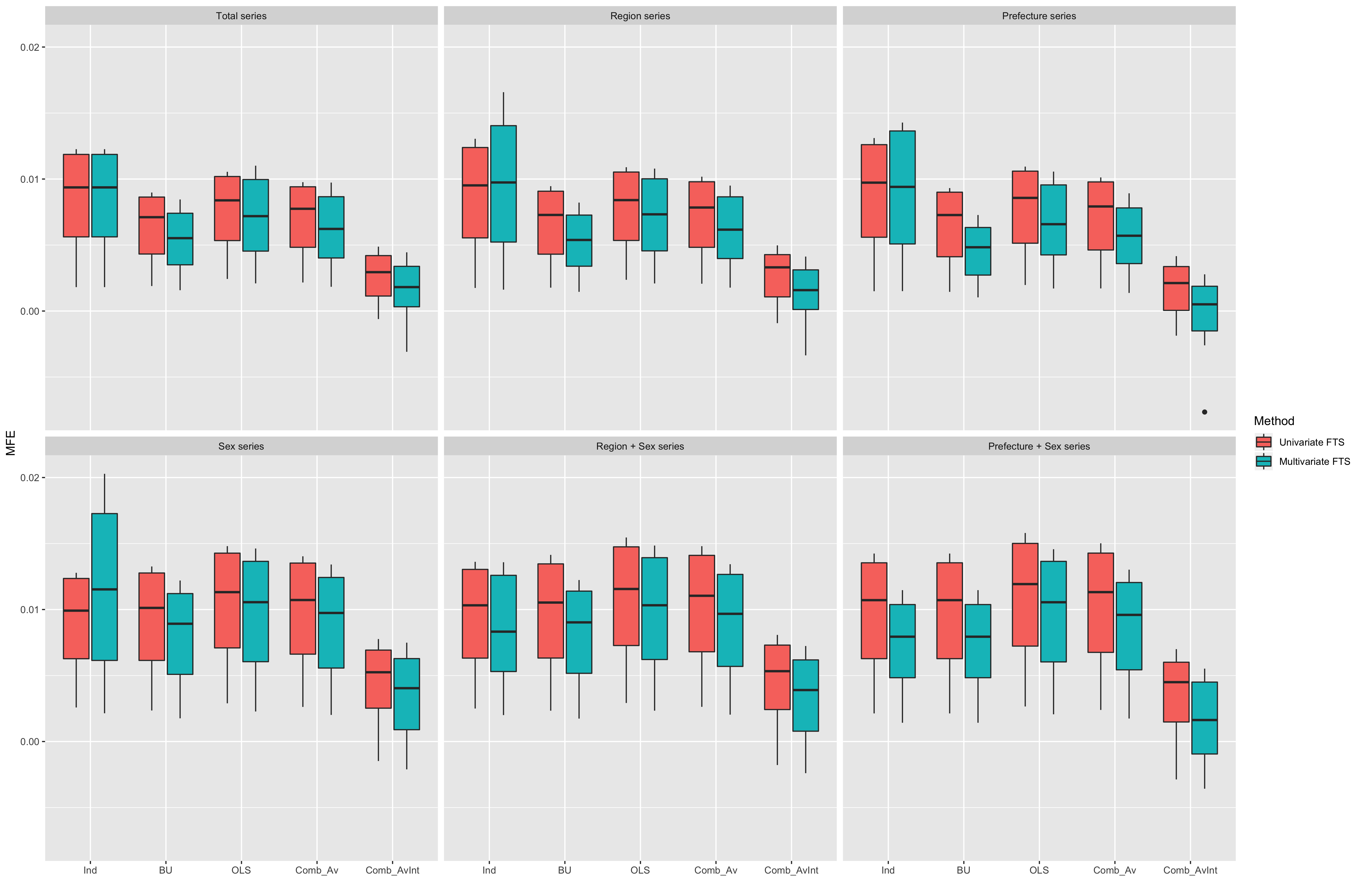
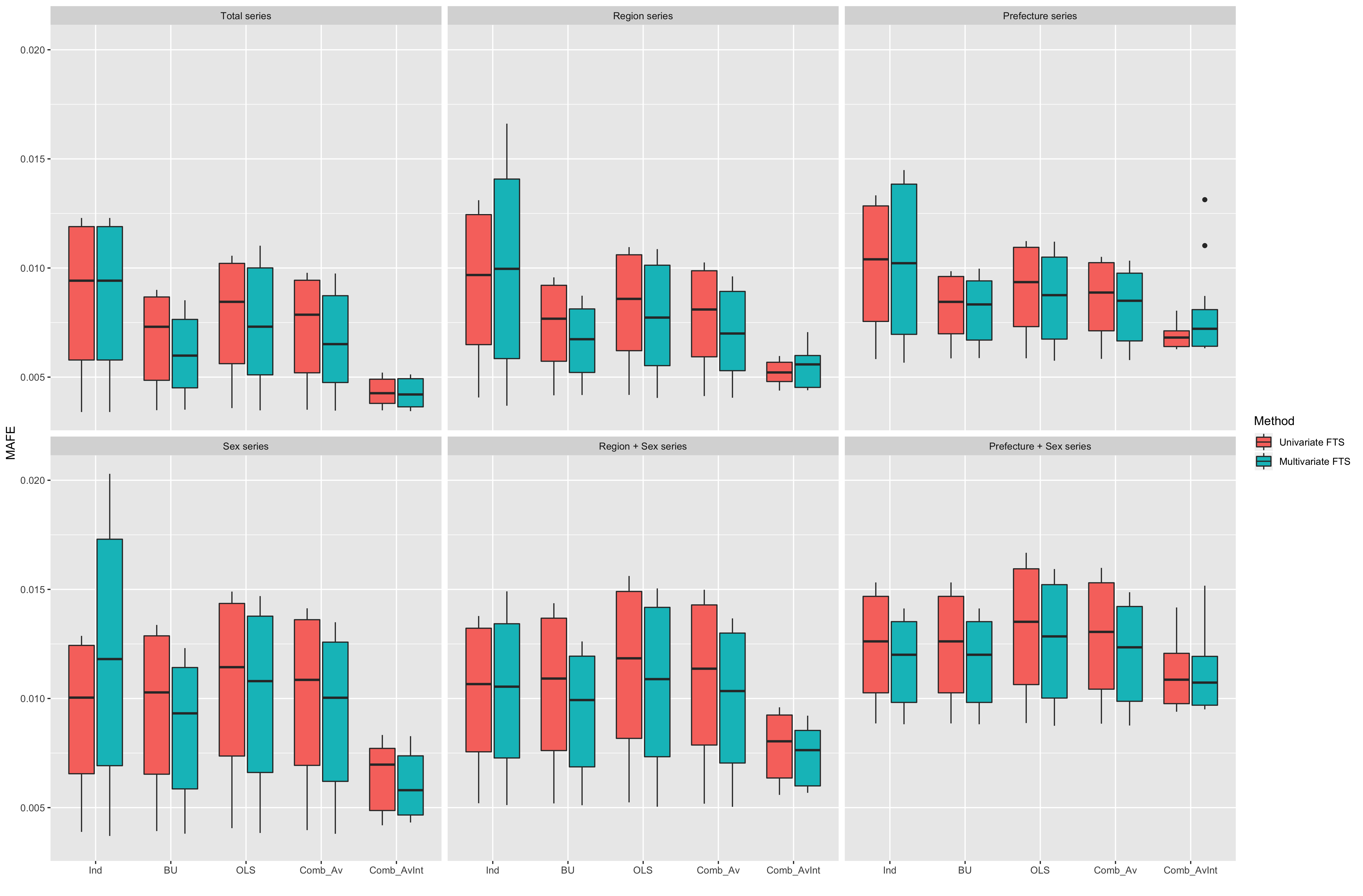
Figure 5 similarly compares MAFE($h$) between the univariate and multivariate functional time-series methods. The multivariate functional time-series method generally produces smaller point forecast errors than the ones obtained using the univariate functional time-series method for almost all levels of the group structure. Based on the two summary statistics of the forecast errors, the multivariate functional time-series method coupled with the forecast combination method (AvInt) performs the best across all levels of the group structure, while it reconciles point forecasts taking account of the group structure. The advantage of this forecast combination is that it can reduce point forecast errors.

We apply the method of Shang 2020 to construct pointwise prediction intervals. To evaluate pointwise interval forecast accuracy, we first construct lower and upper bounds of a prediction interval at the $100(1-\alpha)\%$ nominal coverage probability, where $\alpha$ denotes a significance level (see, Shang and Haberman 2017, for details). Then, we utilize the interval score of Gneiting and Raftery 2007. In the literature, extensive works are available on interval score and will not be reiterated here. The optimal interval score is achieved when there is almost $100(1-\alpha)\%$ of times that the holdout data lie between the upper and lower bounds of the prediction interval, and the distance between the upper and lower bounds is minimal.

Since the number of series is different across different levels of disaggregation, we obtain an overall assessment of interval forecast accuracy by taking the simple average of the interval scores across the number of series at each level. Also, for 15 different forecast horizons, we consider the mean and median values to evaluate overall interval forecast accuracy among the methods for national and sub-national mortality forecasts.

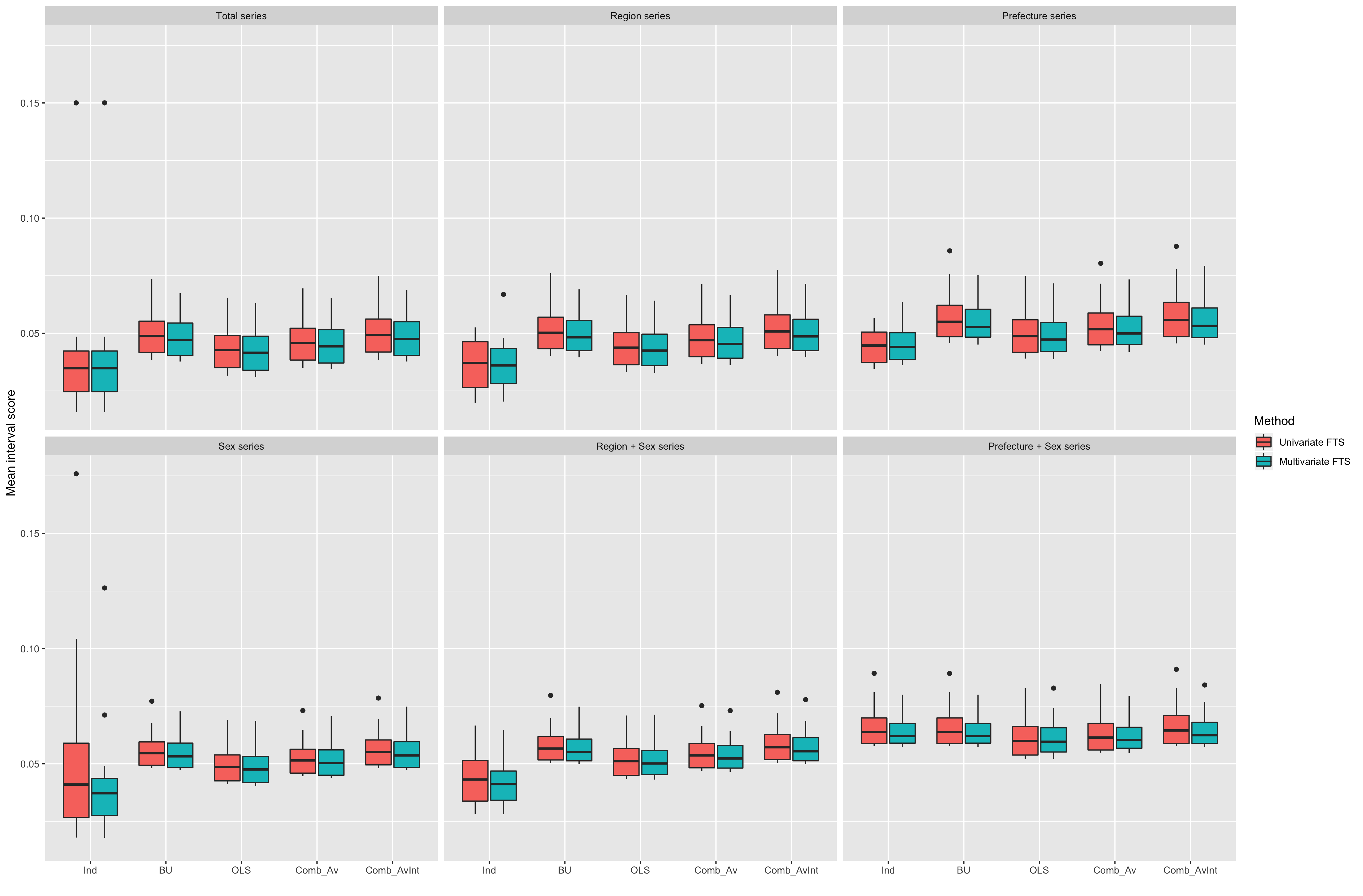
Averaging over all the series at each level of the group structure, Figure 6 presents the mean interval scores $\overline{S}_{\alpha}(h)$ between the univariate and multivariate functional time-series methods. Based on the averaged summary statistics of $\overline{S}_{\alpha}(h)$, the independent forecasting method generally performs the best because it fits each series without the constraint of a hierarchy. At the prefecture level, the optimal-combination method outperforms the independent functional time series forecasting method, which demonstrates the improved interval-forecast accuracy of the optimal-combination method while reconciling interval forecasts. Between the univariate and multivariate functional time-series methods, there is a slight advantage to use the multivariate functional time-series method at each level of the group structure. The forecast combination method with equal weighting produces mean interval scores that lie between the ones of the bottom-up and optimal-combination methods. The forecast combination method with simple averaging of midpoints produces the largest mean interval scores and thus this method is conservative.

References

- (1)
- Bates and Granger (1969) Bates, J. M. and Granger, C. W. J. (1969), ‘The combination of forecasts’, Operational Research Quarterly 20(4), 451–468.
- Cannon and Tonks (2008) Cannon, E. and Tonks, I. (2008), Annuity Markets, Oxford University Press, Oxford.
- Dickson et al. (2009) Dickson, D. C. M., Hardy, M. R. and Waters, H. R. (2009), Actuarial Mathematics for Life Contingent Risks, Cambridge University Press, Cambridge.
- Fung et al. (2017) Fung, M. C., Peters, G. W. and Shevchenko, P. V. (2017), ‘A unified approach to mortality modelling using state-space framework: Characterisation, identification, estimation and forecasting’, Annals of Actuarial Science 11(2), 343–389.
- Gaba et al. (2017) Gaba, A., Tsetlin, I. and Winkler, R. L. (2017), ‘Combining interval forecasts’, Decision Analysis 14(1), 1–74.
- Gaille and Sherris (2015) Gaille, S. A. and Sherris, M. (2015), ‘Causes-of-death mortality: What do we know on their dependence?’, North American Actuarial Journal 19(2), 116–128.
- Gneiting and Raftery (2007) Gneiting, T. and Raftery, A. E. (2007), ‘Strictly proper scoring rules, prediction and estimation’, Journal of the American Statistical Association 102(477), 359–378.
- Hatzopoulos and Haberman (2013) Hatzopoulos, P. and Haberman, S. (2013), ‘Common mortality modelling and coherent forecasts - an empirical analysis of worldwide mortality data’, Insurance: Mathematics and Economics 52(2), 320–337.
- Hyndman et al. (2011) Hyndman, R. J., Ahmed, R. A., Athanasopoulos, G. and Shang, H. L. (2011), ‘Optimal combination forecasts for hierarchical time series’, Computational Statistics and Data Analysis 55(9), 2579–2589.
- Hyndman and Khandakar (2008) Hyndman, R. J. and Khandakar, Y. (2008), ‘Automatic time series forecasting: the forecast package for R’, Journal of Statistical Software 27(3).
- Hyndman and Ullah (2007) Hyndman, R. J. and Ullah, M. S. (2007), ‘Robust forecasting of mortality and fertility rates: A functional data approach’, Computational Statistics & Data Analysis 51(10), 4942–4956.
- Japanese Mortality Database (2019) Japanese Mortality Database (2019), National Institute of Population and Social Security Research, Available at http://www.ipss.go.jp/p-toukei/JMD/index-en.html. data downloaded on July 18, 2018.
- Lee and Carter (1992) Lee, R. D. and Carter, L. R. (1992), ‘Modeling and forecasting U.S. mortality’, Journal of the American Statistical Association 87(419), 659–671.
- Li et al. (2019) Li, H., Li, H., Lu, Y. and Panagiotelis, A. (2019), ‘A forecast reconciliation approach to cause-of-death mortality modeling’, Insurance: Mathematics and Economics 86, 122–133.
- Li and Lee (2005) Li, N. and Lee, R. (2005), ‘Coherent mortality forecasts for a group of populations: An extension of the Lee–Carter method’, Demography 42(3), 575–594.
- Olivieri and Pitacco (2016) Olivieri, A. and Pitacco, E. (2016), ‘Frailty and risk classification for life annuity portfolios’, Risks 4(4), 39.
- O’Meara and Bruhn (2013) O’Meara, T. and Bruhn, A. (2013), ‘Compulsory Annuitisation: A policy option for Australia?’, Australasian Accounting Business and Finance Journal 7(3), 5–30.
- Richman and Wüthrich (2020a) Richman, R. and Wüthrich, M. V. (2020a), ‘A neural network extension of the Lee-Carter model to multiple populations’, Annals of Actuarial Science in press.
- Richman and Wüthrich (2020b) Richman, R. and Wüthrich, M. V. (2020b), Lee and Carter go machine learning: Recurrent neural networks, Working paper, ETH Zurich. Available at SSRN: https://papers.ssrn.com/abstract=3441030.
- Shang (2020) Shang, H. L. (2020), ‘Dynamic principal component regression for forecasting functional time series in a group structure’, Scandinavian Actuarial Journal in press.
- Shang et al. (2011) Shang, H. L., Booth, H. and Hyndman, R. J. (2011), ‘Point and interval forecasts of mortality rates and life expectancy: A comparison of ten principal component methods’, Demographic Research 25(5), 173–214.
- Shang and Haberman (2017) Shang, H. L. and Haberman, S. (2017), ‘Grouped multivariate and functional time series forecasting: An application to annuity pricing’, Insurance: Mathematics and Economics 75, 166–179.
- Shang and Hyndman (2017) Shang, H. L. and Hyndman, R. J. (2017), ‘Grouped functional time series forecasting: An application to age-specific mortality rates’, Journal of Computational and Graphical Statistics 26(2), 330–343.
- Villegas and Haberman (2014) Villegas, A. M. and Haberman, S. (2014), ‘On the modeling and forecasting of socioeconomic mortality differentials: An application to deprivation and mortality in England’, North American Actuarial Journal 18(1), 168–193.
- Wickramasuriya et al. (2019) Wickramasuriya, S. L., Athanasopoulos, G. and Hyndman, R. J. (2019), ‘Optimal forecast reconciliation for hierarchical and grouped time series through trace minimization’, Journal of the American Statistical Association: Theory and Methods 114(526), 804–819.
- Yaari (1965) Yaari, M. E. (1965), ‘Uncertain lifetime, life insurance, and the theory of the consumer’, The Review of Economic Studies 32(2), 137–150.