Quantifying many-body learning far from equilibrium with representation learning
Abstract
Far-from-equilibrium many-body systems, from soap bubbles to suspensions to polymers, learn the drives that push them. This learning has been observed via thermodynamic properties, such as work absorption and strain. We move beyond these macroscopic properties that were first defined for equilibrium contexts: We quantify statistical mechanical learning with machine learning. Our toolkit relies on a structural parallel that we identify between far-from-equilibrium statistical mechanics and representation learning, which is undergone by neural networks that contain bottlenecks, including variational autoencoders. We train a variational autoencoder, via unsupervised learning, on configurations assumed by a many-body system during strong driving. We analyze the neural network’s bottleneck to measure the many-body system’s classification ability, memory capacity, discrimination ability, and novelty detection. Numerical simulations of a spin glass illustrate our technique. This toolkit exposes self-organization that eludes detection by thermodynamic measures, more reliably and more precisely identifying and quantifying learning by matter.
Systems given many degrees of freedom can learn and remember patterns of forces that propel them far from equilibrium. Such behaviors have been predicted and observed in many settings, from charge-density waves Coppersmith_97_Self; Povinelli_99_Noise to non-Brownian suspensions Keim_11_Generic; Keim_13_Multiple; Paulsen_14_Multiple, polymer networks Majumdar_18_Mechanical, soap-bubble rafts Mukherji_19_Strength, and macromolecules Zhong_17_Associative. Such learning holds promise for engineering materials capable of memory and computation. This potential for applications, with experimental accessibility and ubiquity, have earned these classical nonequilibrium many-body systems much attention recently Keim_19_Memory. We measure many-body learning using a neural network (NN) that undergoes representation learning, a type of machine learning. Our toolkit detects and quantifies many-body learning more thoroughly and precisely than thermodynamic measures used to date.
One of the best-characterized instances of learning by driven matter involves a spin glass. The spins are classical and interact randomly. Consider applying fields from a set , which we call a drive. As the driving proceeds, the spins flip, absorbing work. In a certain parameter regime, the absorbed power shrinks adaptively: The spins migrate toward a corner of configuration space where their configuration withstands the drive’s insults. Consider then imposing fields absent from the original drive. Subsequent spin flips will absorb more work than if the field belonged to the original drive. Insofar as a simple, low-dimensional property of the material can be used to discriminate between drive inputs that fit a pattern and drive inputs that do not, we say that the material has learned the drive.
Learning behavior has been quantified with properties commonplace in thermodynamics. Examples include work, magnetization, and strain. This thermodynamic characterization has provided insights but suffers from two shortcomings. First, the types of thermodynamic properties vary from system to system. For example, work absorption characterizes the spin glass’s learning; strain characterizes polymer networks’. A more general approach would facilitate comparisons and standardize analyses. Second, thermodynamic properties are useful for characterizing macroscopic equilibrium states. But such properties are not necessarily the best for describing the far-from-equilibrium systems that learn.
Over the past several years, machine learning has revolutionized the quantification of learning Nielsen_15_Neural; Goodfellow_16_Deep. Machine learning calls for application to the learning of drive patterns by many-body systems.
Parallels between statistical mechanics and certain machine-learning components have been known for decades Engel_01_Statistical; Nielsen_15_Neural. For example, Boltzmann machines resemble particles exchanging heat with thermal baths. Parallels between representation learning and statistical mechanics have enjoyed less attention (though one parallel was proposed in Alemi_18_TherML). Figure 1(a) illustrates representation learning Bengio_12_Representation: A high-dimensional variable is inputted into a NN. The NN compresses relevant information into a low-dimensional variable . The NN then decompresses into a prediction of a high-dimensional variable . If , the NN is an autoencoder, mimicking the identity function. The latent variable acts as a bottleneck. The bottleneck’s size controls a tradeoff between the memory consumed and the prediction’s accuracy. We call the NNs that perform representation learning bottleneck NNs.
Representation learning, we argue, shares its structure with problems in which a strong drive forces a many-body system [Fig. 1(b)]. The system’s microstate, like , occupies a high-dimensional space. A macrostate synopsizes the microstate in a few numbers, such as particle number and magnetization. This synopsis parallels . If the system has learned the drive, the macrostate encodes the drive. One may reconstruct the drive from the macrostate, as a bottleneck NN reconstructs from .
Applying this analogy, we use representation learning to measure how effectively a far-from-equilibrium many-body system learns a drive. We illustrate with numerical simulations of the spin glass, whose learning has been characterized with work absorption Gold_19_Self. However, our methods generalize to other platforms. Our measurement scheme offers three advantages:
- 1.
Bottleneck NNs register learning behaviors more thoroughly, reliably, and precisely than work absorption.
- 2.
Our framework applies to a wide class of strongly driven many-body systems. The framework does not rely on strain, work absorption, susceptibility, etc. Hence our toolkit can characterize spins, suspensions, polymers, etc.
- 3.
Our approach unites a machine-learning sense of learning with the statistical mechanical sense. This union is conceptually satisfying.
We apply representation learning to measure classification, memory capacity, discrimination, and novelty detection. Our techniques can be extended to other facets of learning, such as prediction and the decomposition of a drive into constituents.
Most of our measurement schemes have the following structure: The many-body system is trained with a drive (e.g., fields , , and ). Then, the system is tested (e.g., with a field ). Training and testing are repeated in many trials. Configurations realized are used to train a bottleneck NN. In some cases, the NN then receives data from the statistical mechanical testing. Finally, we analyze the NN’s latent space and/or predictions.
The rest of this paper is organized as follows. Section I introduces the bottleneck NN that we use and the spin-glass example. In Sec. II, we prescribe how to quantify, using representation learning, the learning of a drive by a many-body system. Section III closes with a discussion: We decode our NN’s latent space in terms of thermodynamic variables, argue for our techniques’ feasibility, and detail opportunities engendered by this study.
I Setup: Representation-learning model and spin-glass example
This section introduces two toolkits applied in Sec. II: (i) Section I A details the bottleneck NN we use. (ii) Section I B details the spin glass with which we illustrate statistical mechanical learners.
I A Representation-learning model
This section overviews our architecture; details appear in App. A. This paper’s introduction identifies a parallel between thermodynamic problems and bottleneck NNs (Fig. 1). In the thermodynamic problem, represents the drive. We could design a bottleneck NN that predicts drives from configurations . But the NN would need to undergo supervised learning, if built according to today’s standards. During supervised learning, the NN would receive tuples (configuration, label of drive that generated the configuration). Receiving drive labels would give the NN information not directly accessible to the many-body system. The NN’s predictive success would not necessarily reflect only learning by the many-body system. Hence we design a bottleneck NN that performs unsupervised learning, receiving just configurations.
This NN is a variational autoencoder (VAE) Kingma_13_Auto; JR_14_Stochastic; Doersch_16_Tutorial. A VAE is a generative model: It receives samples from a distribution over the possible values of , learns about the distribution, and generates new samples. The NN approximates the distribution, using Bayesian variational inference (App. A). The parameters are optimized during training facilitated by backpropagation.
Our VAE has five fully connected hidden layers, with neuron numbers 200-200-(number of neurons)-200-200. We usually restrict to 2-4 neurons. This choice facilitates the visualization of the latent space and suffices to quantify our spin glass’s learning. Growing the number of degrees of freedom, and the number of drives, may require more dimensions. But our study suggests that the number of dimensions needed the system size.
The latent space is visualized in Fig. 2. Each neuron corresponds to one axis and represents a continuous-valued real number. The VAE maps each inputted configuration to one latent-space dot. Close-together dots correspond to configurations produced by the same field, if the spin glass and NN learn well. We illustrate this clustering in Fig. 2 by coloring each dot according to the drive that produced it.
I B Spin glass
A spin glass exemplifies the statistical mechanical learner. We introduce the spins, Hamiltonian, and heat exchange below. We model the time evolution, define work and heat, and describe the initialization procedure. Finally, we describe a parameter regime in which the spin glass learns effectively. Appendix B distinguishes robust learning from superficially similar behaviors.
We adopt the model in Gold_19_Self. Simulations are of classical spins. The spin occupies one of two possible states: .
The spins couple together and experience an external magnetic field. Spin evolves under a Hamiltonian
| (1) |
and the spin glass evolves under
| (2) |
at time . We call the first term in Eq. (1) the interaction energy and the second term the field energy. The couplings are defined in terms of an Erdös-Rényi random network: Nodes and have some probability of sharing an edge, for all and . We identify nodes with spins and identify edges with couplings. Each spin couples to eight other spins, on average. The nonzero couplings are selected according to a normal distribution of standard deviation 1.
The in Eq. (1) is defined as follows. At time , the spin glass experiences a field . represents the magnitude and sign of the field at spin . All fields point along the same direction (conventionally labeled as the -axis), so we simplify the vector notation to . Elsewhere in the text, we simplify to the capital Latin letter (or , or , etc.). Each is selected according to a normal distribution of standard deviation 3. The field changes every 100 seconds. To train the spin glass, we construct a drive by forming several random fields . We randomly select a field from the set, then apply the field. We repeat these two steps 299 times, unless otherwise noted (Fig. 3).
The spin glass exchanges heat with a bath at a temperature . We set Boltzmann’s constant to one: . Energies are measured in units of Kelvins (K). To flip, a spin must overcome an energy barrier of height . Spin tends to flip at a rate
| (3) |
Equation (3) has the form of Arrhenius’s law and obeys detailed balance. Each spin flips once every s, on average. We model the evolution with discrete 100-s time intervals, using the Gillespie algorithm.
The spins absorb work when the field changes, and they dissipate heat while flipping, as we now detail. Consider changing the field from to . The change in the spin glass’s energy equals the work absorbed by the spin glass:
| (4) |
To define heat, we suppose that spin flips at time : . The spin glass dissipates an amount of heat equal to the negative of the change in the spin glass’s energy:
| (5) | ||||
| (6) |
Our discussion is cast in terms of the absorbed power, .
The spin glass is initialized in a uniformly random configuration . Then, the spins relax in the absence of any field for 100,000 seconds. The spin glass navigates to near a local energy minimum. If a protocol is repeated in multiple trials, all the trials begin with the same .
In a certain parameter regime, the spin glass learns its drive effectively, even according to the absorbed power Gold_19_Self. Consider training the spin glass on a drive . The spin glass absorbs much work initially. If the spin glass learns the drive, the absorbed power declines. If a dissimilar field is then applied, the absorbed power spikes. The spin glass learns effectively when K-1 and K Gold_19_Self. These parameters define a Goldilocks regime: The temperature is high enough, and the barriers are low enough, that the spin glass can explore phase space. But is low enough, and the barriers are high enough, that the spin glass is not hopelessly peripatetic.
II How to detect and quantify
a many-body system’s
learning of a drive,
using representation learning
This section shows how to quantify four facets of learning. Section II A concerns the many-body system’s ability to classify drives; Sec. II B, memory capacity; Sec. II C, discrimination of similar fields; and Sec. II D, novelty detection. At the end of each section, we synopsize the technique introduced in boldface. These four techniques illustrate how representation learning can be applied to quantify features of learning. Other features may be quantified along similar lines. Code used can be found at the online repository Github_repo.
II A Classification: Which drive is this?
A system classifies a drive by identifying the drive as one of many possibilities. A VAE, we find, reflects more of a spin glass’s classification ability than absorbed power does.
We illustrate with the spin glass. We generated random fields , , , , and . From 4 of the fields, we formed the drive . On the drive, we trained the spin glass in each of 1,000 trials. In each of 1,000 other trials, we trained a fresh spin glass on a drive . We repeated this process for each of the 5 possible 4-field drives. Ninety percent of the trials were randomly selected for training our NN. The rest were used for testing.
We used the VAE to gauge the spin glass’s classification of the drives: We identified the configurations occupied by the spin glass at a fixed time in the training trials. On these configurations, we trained the VAE. The VAE populated the latent space with dots (as in Fig. 2) whose density formed a probability distribution.
We then showed the VAE a time- configuration from a test trial. The VAE compressed the configuration into a latent-space point. We calculated which drive most likely, according to the probability density, generated the latent-space point. The calculation was maximum a posteriori estimation (MAP estimation) (see Bishop_06_Pattern and App. C). Here, the MAP estimation is equivalent to maximum-likelihood estimation. We performed this testing and estimation for each trial in the test data. The fraction of trials in which MAP estimation succeeded forms the score. We scored the classification at each of many times . The score is plotted against in Fig. 4, as the blue, upper curve.
The absorbed power reflects the spin glass’s classification of the drives as follows. For each drive and each time , we histogrammed the power absorbed while was applied at in a VAE-training trial. Then, we took a trial from the test set and identified the power absorbed at . We inferred which drive most likely, according to the histograms, produced . The guess’s score appears as the orange, lower curve in Fig. 4.
The score maximizes at 1.00 if the drive is always guessed accurately. The score is lower-bounded by , which results from random guessing. In Fig. 4, each score grows over a time scale of tens of field switches. The absorbed-power score begins at 0.2011 1 The VAE’s score begins close to 0.20. The slight distance from 0.20, we surmise, comes from stochasticity of three types: the spin glass’s initial configuration, the MAP estimation, and stochastic gradient descent. Stochasticity of only the first two types affects the absorbed power’s score. and comes to fluctuate around 0.25. The VAE’s score comes to fluctuate slightly below 1.00. Hence the VAE reflects more of the spin glass’s classification ability than the absorbed power does.
A many-body system’s ability to classify drives is quantified with the score of MAP estimates calculated from a VAE’s latent space.
II B Memory capacity: How many drives can be remembered?
How many fields can a many-body system remember? A VAE, we find, registers a greater capacity than absorbed power registers.22 2 We use the term “memory capacity” in the physical sense of Keim_19_Memory. A more specific, technical definition of “memory capacity” is used in reservoir computing Jaeger_02_Short. Hence the VAE reflects statistical mechanical learning, at high field numbers, that the absorbed power does not.
We illustrated by constructing 50 random fields. We selected 40 to form a drive , selected 40 to form a drive , and repeated until forming 5 drives. We trained the spin glass on in each of 1,000 trials, for each of . Ninety percent of the trials were designated as VAE-training trials; and 10%, as VAE-testing trials.
The choice of 50 fields is explained in App. D: Fifty fields exceed the spin-glass capacity registered by the absorbed power. We aim to show that 50 fields do not exceed the capacity registered by the VAE: The VAE identifies spin-glass learning missed by the absorbed power.
We used representation learning to quantify the spin glass’s capacity as follows. For a fixed time , we collected the configurations occupied by the spin glass at in the VAE-training trials. On these configurations, the VAE performed unsupervised learning. The VAE populated its latent space with dots that formed five clusters. Then, we fed the VAE the configuration occupied at during a test trial. The VAE formed a new dot in latent space. We MAP-estimated the drive that, according to the VAE, most likely generated the dot (Sec. II A). The fraction of test trials in which the VAE guessed correctly constitutes the VAE’s score. The score is plotted against in Fig. 5, as the blue, upper curve.
The VAE’s score is compared with the absorbed power’s score, calculated as follows. For a fixed time , we identified the power absorbed at in each VAE-testing trial. We histogrammed the power absorbed when was applied at , for each . We then identified the power absorbed at in a test trial. Comparing with the histograms, we inferred which drive was most likely being applied. We repeated this inference with each other test trial. In which fraction of the trials did the absorbed power identify the drive correctly? This number forms the absorbed power’s score. The score is plotted as the lower, orange curve in Fig. 5.
The higher the score, the greater the memory capacity attributed to the spin glass. The absorbed power identifies the drive in approximately of the trials, as would random guessing. The score remains approximately constant, because the number of fields exceeds the spin-glass capacity measured by the absorbed power. In contrast, the VAE’s score grows over changes of the field, then plateaus at . The VAE points to the wrong drive most of the time but succeeds significantly more often than the absorbed power. Hence representation learning uncovers more of the spin glass’s memory capacity than absorbed power measure does.
A many-body system’s memory capacity is quantified with the greatest number of fields in any drive on which MAP estimation, based on a VAE’s latent space, scores better than random guessing.
II C Discrimination: How new is this field?
Suppose that a many-body system learns fields and , then encounters a field that interpolates between them. Can the system recognize that the new field contains familiar constituents? Can the system discern how much contributes and how much contributes? The answers characterize the system’s discrimination ability, which we quantify with a MAP-estimation score (Sec. II A). Estimates formed from a VAE’s latent space reflect more of the system’s discriminatory ability than do estimates formed from absorbed power.
We illustrate with the spin glass, forming a drive . In each of 300 time intervals, a field was selected randomly from the drive and applied. The spin glass was then tested with a linear combination . The weight varied from 0 to 1, in steps of , across trials.
We measured the spin glass’s discrimination using the VAE as follows. The final configuration assumed by the spin glass in each test trial was collected. The configurations were split into VAE-training data and VAE-testing data. On the configurations generated by in the VAE-training data, the VAE was trained. Then, the VAE received a configuration generated by in a VAE-testing trial. The VAE mapped the configuration to a latent-space point. We inferred which field most likely generated that point, using MAP estimation on the latent space. We tested the VAE many times, then calculated the fraction of MAP estimates that were correct, the VAE’s score.
Similarly, we measured the spin glass’s discrimination using the absorbed power. For each trial in the VAE-training data, we calculated the power absorbed by the spin glass after the application of . We histogrammed , inferring the probability that, if shown for a given , the spin glass will absorb an amount of power. Then, we calculated the power absorbed during a VAE-testing trial. We inferred which field most likely generated that point, using MAP estimation on the latent space. Repeating MAP estimation with all the VAE-testing trials, we calculated the absorbed power’s score.
The VAE’s score equals about double the absorbed power’s score, for latent spaces of dimensionality 2 to 20. The VAE scores between 0.448 and 0.5009, whereas the absorbed power scores 0.2381. Hence the representation-learning model picks up on more of the spin glass’s discriminatory ability than the absorbed power does.
A many-body system’s ability to discriminate combinations of familiar fields is quantified with the score of MAP estimates formed from a VAE’s latent space.
II D Novelty detection: Has this drive been encountered before?
At the start of the introduction, we described how absorbed power has been used to identify novelty detection. A system detects novelty when labeling a stimulus as familiar or unfamiliar. The stimulus produces a response that exceeds a threshold or lies below. If the stimulus exceeds the threshold, an observer should guess that the stimulus is novel. Otherwise, the observer should guess that the stimulus is familiar.
The observer can err in two ways: One commits a false positive by believing a familiar drive to be novel. One commits a false negative by believing a novel drive to be familiar. The errors trade off: Raising the threshold lowers the probability , suppressing false positives at the cost of false negatives. Lowering the threshold lowers the probability , suppressing false negatives at the cost of false positives.
The receiver-operating-characteristic (ROC) curve depicts the tradeoff’s steepness (see Brown_06_Receiver and Fig. 6). Each point on the curve corresponds to one threshold value. The false-positive rate runs along-the -axis; and the true-positive rate, , along the -axis. The greater the area under the ROC curve, the more sensitively the response reflects accurate novelty detection.
We measure a many-body system’s novelty-detection ability using an ROC curve. Let us illustrate with the spin glass. We constructed two random drives, and . We trained the spin glass on . In each of 3,000 trials, we then tested the spin glass with , , or . In each of 3,000 other trials, we tested with , , or . We defined one response in terms of a VAE, as detailed below; measured the absorbed power, a thermodynamic response; and, from each response, drew an ROC curve (Fig. 6). The curves show that representation learning offers greater sensitivity to the spin glass’s novelty detection.
We defined the representation-learning response in terms of a VAE as follows. We trained the VAE on the configurations assumed by the spin glass during its training. The VAE populated latent space with three clumps of dots. We modeled the clumps with a hard mixture of three Gaussians.33 3 A mixture is hard if it models each point as belonging to only one Gaussian. We then fed the VAE the configuration that resulted from testing the spin glass. The VAE mapped the configuration to a latent-space point . We calculated the probability that the distribution produced the new point. This protocol led to the blue, solid curve in Fig. 6.
We defined a thermodynamic ROC curve in terms of absorbed power. Consider the trials in which the spin glass is tested with field . We histogrammed the power absorbed by the spin glass at the end of the testing. We form another histogram from the -test trials; and a third histogram, from the -test trials. To these histograms was compared the power that the spin glass absorbed during a test with an arbitrary field. We inferred the likelihood that resulted from a familiar field. The results form the orange, dashed curve in Fig. 6.
The two ROC curves enclose regions of approximately the same area: The VAE curve encloses an area-0.9633 region; and the thermodynamic curve, an area-0.9601 region. On average across all thresholds, therefore, the responses register novelty detection approximately equally. Yet the responses excel in different regimes: The VAE achieves greater true-positive rates at low false-positive rates, and the absorbed power achieves greater true-positive rates at high false-positive rates. This two-regime behavior persisted across batches of trials, though the enclosed areas fluctuated a little. Hence anyone paranoid about avoiding false positives should measure a many-body system’s novelty detection with a VAE, while those more relaxed might prefer the absorbed power.
Why should the VAE excel at low false-positive rates? Because of the VAE’s skill at generalizing, we conjecture. Upon training on cat pictures, a VAE generalizes from the instances. Shown a new cat, the VAE recognizes its catness. Perturbing the input a little perturbs the VAE’s response little. Hence changing the magnetic field a little, which changes the spin-glass configuration little, should change latent space little, obscuring the many-body system’s novelty detection. This obscuring disappears when the magnetic field changes substantially.
A many-body system’s novelty-detection ability is quantified with an ROC curve formed from a VAE’s latent space or a thermodynamic response, depending on the false-positive threshold.
III Discussion
We have detected and quantified a many-body system’s learning of its drive, using representation learning, with greater sensitivity than absorbed power affords. The scheme relies on a parallel that we identified between statistical mechanical problems and VAEs. Uniting statistical mechanical learning with machine learning, the definition is conceptually satisfying. The definition also has wide applicability, not depending on whether the system exhibits magnetization or strain or another thermodynamic response. Furthermore, our representation-learning toolkit signals many-body learning more sensitively than does the seemingly best-suited thermodynamic tool.
The rest of this section is organized as follows. In Sec. III A, we decode latent space in terms of thermodynamic variables. In Sec. III B, we argue for the feasibility of applying our toolkit. In Sec. III C, we discuss problems that our toolkit can illuminate. We also motivate the development of new representation-learning tools.
III A Decoding latent space
Thermodynamicists parameterize macrostates with volume, energy, magnetization, etc. Thermodynamic macrostates parallel latent space, as illustrated in Fig. 1. What variables parameterize the VAE’s latent space? Latent space could suggest definitions of new thermodynamic variables, or hidden relationships amongst known thermodynamic variables. We begin decoding latent space in terms of thermodynamic quantities, leaving the full decoding for future research.
We illustrate with part of the spin-glass protocol in Sec. II A: Train the spin glass with a drive in each of many trials. On the end-of-trial configurations, train the VAE.


Figure 7 shows two visualizations of the latent space. Each visualization spotlights a correlation between a latent-space direction and a thermodynamic variable. In Fig. 7(a), blue dots represent configurations in which the spin glass absorbs little work. Red dots highlight high-absorbed-power configurations. The dots change from blue to red along the diagonal from the lower right-hand corner to the upper left-hand. Hence a point’s distance along the diagonal correlates with the absorbed power.
In Fig. 7(b), blue represents low magnetizations, and red represents high. Blue dots cluster near the latent space’s center, and red dots occupy the outskirts. Hence magnetization correlates with a dot’s radial coordinate. Magnetization correlates, to some extent, also with distance along the bottom-right-to-upper-left diagonal. After all, magnetization is related to the absorbed power.
In summary, the diagonal corresponds roughly to the absorbed power, and the radial direction corresponds roughly to magnetization. The directions are nonorthogonal, suggesting a nonlinear relationship between the thermodynamic variables. We leave the parameterization of the relationship, and the possible decoding of other latent-space directions into new thermodynamic variables, for future work.
III B Feasibility
Applying our toolkit might appear impractical, since microstates must be inputted into the NN. Measuring a many-body system’s microstate may daunt experimentalists. Yet the use of microstates hinders our proposal little, for three reasons.
First, microstates can be calculated in numerical simulations, which inform experiments. Second, many key properties of many-body microstates have been measured experimentally. High-speed imaging has been used to monitor soap bubbles’ positions Mukherji_19_Strength and colloidal suspensions Cheng_11_Imaging. Similarly wielded tools, such as high magnification, have advanced active-matter Sanchez_12_Spontaneous and gene-expression Lonsdale_13_Genotype studies.
One might worry that the full microstate cannot be measured accurately or precisely. Soap bubbles’ positions can be measured with finite precision, and other microscopic properties might be inaccessible. But, third, some bottleneck NNs denoise their inputs Vincent_08_Extracting; Goodfellow_16_Deep: The NNs learn the distribution from which samples are generated ideally, not systematic errors. Denoising by VAEs is less established but is progressing Im_15_Denoising.
Furthermore, one might wonder whether our study requires deep learning. Could simpler algorithms detect and measure many-body learning as sensitively? Appendix E addresses this question. We compare the VAE with simpler competitors that perform unsupervised learning: a single-layer linear NN, related to principal-component analysis (PCA) Bourland_88_Auto, and a clustering algorithm. The VAE outperforms both competitors.
III C Opportunities
Several opportunities emerge from this combination of statistical mechanical learning and bottleneck NNs. First, our toolkit may resolve open problems in the field of statistical mechanical learning. One example concerns the soap-bubble raft in Mukherji_19_Strength. Experimentalists trained a raft of soap bubbles with an amplitude- strain. The soap bubbles’ positions were tracked, and variances in positions were calculated. No such measures distinguished trained rafts from untrained rafts; only stressing the raft and reading out the strain could Mukherji_19_Strength; Miller_19_Raft. Bottleneck NNs may reveal what microscopic properties distinguish trained from untrained rafts.
Similarly, representation learning might facilitate the detection of active matter. Self-organization is detected now through simple, large-scale, easily visible signals Heylighen_02_Science. Bottleneck NNs could identify patterns invisible in thermodynamic measures.
Second, our framework calls for extensions to quantum systems. Far-from-equilibrium many-body systems have been realized with many quantum platforms, including ultracold atoms Langen_15_Ultracold, trapped ions Friis_18_Observation; Smith_16_Many, and nitrogen vacancy centers Kucsko_18_Critical. Applications to memories have been proposed Abanin_19_Colloquium; Turner_18_Weak. Yet quantum memories that remember particular coherent states have been focused on. The learning of strong drives by quantum many-body systems calls for exploration, as the learning of strong drives by polymers, soap bubbles, etc. has proved so productive in classical statistical mechanics. Our framework can guide this exploration.
Third, we identified a parallel between representation learning and statistical mechanics. The parallel enabled us to use representation learning to gain insight into statistical mechanics. Recent developments in information-theoretic far-from-equilibrium statistical mechanics (e.g., Still_12_Thermodynamics; Parrondo_15_Thermodynamics; Crutchfield_17_Origins; Kolchinsky_17_Dependence) might, in turn, shed new light on representation learning.
Fourth, the mutual information between configuration and drive can be calculated as a function of time. Let denote the joint probability that the configuration and the drive . Let and denote the marginal distributions. The mutual information quantifies the information about the drive in the configuration and vice versa: . The mutual information is expected to grow as the many-body system learns. Estimating proved difficult due to undersampling; hence our use of the MAP-estimate score (Sec. II A), a cousin of the mutual information (App. C). This work motivates the development of techniques for estimating from little data.
Such techniques could be complemented by a sampling strategy based on our VAE, fifth. The VAE populates latent space, analogous to the space of macrostates, as in Fig. 2. Consider choosing an unpopulated point, analogous to an unfamiliar macrostate, and having the VAE decompress the point. The VAE will construct a configuration. Such configurations could improve estimates and so estimates. Rough initial studies suggest that the constructed configurations resemble the true samples that they should mimic.
Sixth, given , one can benchmark the many-body system against the information curve Tishby_00_Information. The information curve quantifies the tradeoff in representation learning: Recall the general bottleneck NN described in the introduction. The NN compresses into , then decompresses into [Fig. 1(a)]. The more the NN compresses , the less space requires. Hence shrinking is desirable. Yet must carry enough information about to generate an accurate prediction . Hence should be large. One can tune the mutual informations’ relative importance, using a parameter . One chooses a , then maximizes the objective function . This strategy is called the information bottleneck Tishby_99_Information. Consider varying . At each value, the optimal can be plotted against the optimal . The resulting information curve represents an ideal: Physical systems can reach the points inside the curve, not points outside. Consider plotting a many-body system’s as a point. The point’s distance from the information curve will quantify how close the many-body system approaches to the ideal.
Seventh, we partially decoded the VAE’s latent space in terms of thermodynamic variables (Sec. III A). Further analysis merits exploration. Convention biases thermodynamicists toward measuring volume, magnetization, heat, work, etc. The VAE might identify new macroscopic variables better-suited to far-from-equilibrium statistical mechanics, or hidden nonlinear relationships amongst thermodynamic variables. A bottleneck NN could uncover new theoretical physics, as discussed in, e.g., Carleo_19_Machine; Wu_19_Toward; Iten_20_Discovering.
Acknowledgements.
The authors thank Alexander Alemi, Isaac Chuang, Emine Kucukbenli, Nick Litombe, Seth Lloyd, Julia Steinberg, Tailin Wu, and Susanne Yelin for useful discussions. WZ is supported by ARO Grant W911NF-18-1-0101; the Gordon and Betty Moore Foundation Grant, under No. GBMF4343; and the Henry W. Kendall (1955) Fellowship Fund. JMG is funded by the AFOSR, under Grant FA9950-17-1-0136. SM was supported partially by the Moore Foundation, via the Physics of Living Systems Fellowship. This material is based upon work supported by, or in part by, the Air Force Office of Scientific Research, under award number FA9550-19-1-0411. JLE has been funded by the Air Force Office of Scientific Research grant FA9550-17-1-0136 and by the James S. McDonnell Foundation Scholar Grant 220020476. NYH is grateful for an NSF grant for the Institute for Theoretical Atomic, Molecular, and Optical Physics at Harvard University and the Smithsonian Astrophysical Observatory. NYH also thanks CQIQC at the University of Toronto, the Fields Institute, and Caltech’s Institute for Quantum Information and Matter (NSF Grant PHY-1733907) for their hospitality during the development of this paper.Appendix A Details about the variational autoencoder
We briefly motivate and review VAEs, then describe the VAE applied in the main text. Further background about VAEs can be found in Kingma_13_Auto; JR_14_Stochastic; Doersch_16_Tutorial. We denote vectors with boldface in this appendix.
Denote by data that has a probability of assuming the value . denotes a parameter, and is called the evidence. We do not know the form of , when using representation learning. We model by identifying latent variables that assume the possible values . Let denote the conditional probability that , given that . We model the evidence, using the latent variables, with
| (A1) |
can be related to the posterior distribution . The posterior is the probability that, if , then . By Bayes’ rule, . Calculating the posterior is usually impractical, as is typically intractable (cannot be calculated analytically). Hence we approximate the posterior with a variational model . The optimization parameter denotes the NN’s weights and biases.
The approximation introduces an inference error, quantified with the Kullback-Leibler (KL) divergence. Let and denote distributions over the possible values of a variable. The KL divergence quantifies the distance between the distributions:
| (A2) | ||||
| (A3) |
We denote by the expectation value of a function . Operationally, the KL divergence equals the maximal efficiency with which the distributions can be distinguished, on average, in a binary hypothesis test. We quantify our inference error with the KL divergence between the variational model and the posterior, .
Recall that we wish to estimate : An accurate estimate lets us predict accurately. We wish also to estimate the latent posterior distribution, . We therefore write out the KL divergence’s form, apply Bayes’ rule to rewrite the , rearrange terms, and repackage terms into a new KL divergence:
| (A4) |
The penultimate term encodes our first goal; and the final term, our second goal.
Recall that the KL divergence is nonnegative. The sum of the final two terms therefore lower-bounds the log-likelihood, . denotes the event observed, denotes a possible cause, and denotes the likelihood that caused . Maximizing each side of Eq. (A4), and invoking Ineq. (A3), yields
| (A5) |
The RHS is called the evidence lower bound (ELBO).
A VAE is a neural network that implements the ELBO. encodes the input , and decodes. The VAE has the cost function
| (A6) |
denotes the distribution inferred from the empirical dataset. Given input values , the VAE generates a latent distribution . We denote by the standard multivariate normal distribution whose vector of means is and whose covariance matrix is . Neural-network layers parameterize the VAE’s and . Latent vectors are sampled according to , then decoded into outputs distributed according to . Neural-network layers parameterize the mean vector . The variance is a hyperparameter.
A VAE with the following architecture produced the results in the main text. The style was borrowed from Hafner_18_Building. Two fully connected -neuron hidden layers process the input data. One fully connected two-neuron hidden layer parameterizes each of and . Two fully connected -neuron hidden layers process the latent variables. An output layer reads off the outputs. We choose and use Rectified Linear Unit (ReLU) activations for all hidden layers.
Appendix B Distinction between robust learning
and two superficially similar behaviors
Learning contrasts with two other behaviors that the spin glass could exhibit, entraining to the field and near-freezing.
B 1 Entraining to the field
Imagine that most spins align with any field . The configuration reflects the field as silly putty reflects the print of a thumb pressing on the silly putty. Smoothing the silly putty’s surface wipes the thumbprint off. Similarly, applying a field to the spin glass wipes the signature of from the configuration. From the perspective of the end of the application of , the spin glass has not learned . The spin glass lacks a long-term memory of the field; the field is encoded in no robust, deep properties of the configuration.
We can distinguish learning from entraining by calculating the percentage of the spins that align with the field at the end of training. If the spins obeyed the field, 100% would align. If the spins ignored the field, would align, on average. Hence the spin glass’s entraining is quantified with
| (B1) |
(This measure does not apply to alignment percentages , which are unlikely to be realized.)
Figure 8 shows data collected about the spin glass in the good-learning regime (Sec. I B). The number of aligned spins is plotted against the amount of time for which the spin glass has trained. After the application of one field, 55% of the spins align with the field. At the end of training, 62% align. Hence the spins’ entraining grows from 10% to 24%. Growth is expected, as the spin glass learns the training drive. But is an order of magnitude less than , so the spin glass is not entrained to the field.
B 2 Near-freezing
Suppose that the spin glass is nearly frozen. Most spins cannot flip, but a few jiggle under most fields. The spin glass does not learn any field effectively, being mostly immobile. But the few flippable spins reflect the field. A bottleneck NN could guess the field from those few spins. The NN’s low loss function would induce a false positive, leading us to believe that the spin glass had learned.
We can avoid false positives by measuring two properties. First, we measure the percentage of the spins that antialign with the field. If the percentage consistently , many of the spins are not frozen. Figure 8 confirms that many are not.

Second, we check that the VAE compresses information about spins that have many different field energies [Eq. (1)]. We illustrate with the protocol used to generate Fig. 7: We trained the spin glass on a drive in each of many trials. On the end-of-trial configurations, the VAE was trained.
A configuration is represented in the VAE’s input layer, a column vector. A weight matrix transforms the input layer into the first hidden layer, another column vector. The weight matrix is depicted in Fig. 9. The matrix’s numerical entries have been replaced with colors. Each vertical stripe corresponds to one spin. The farther leftward a stripe, the lesser the spin’s field energy. The darker a stripe, the more information about the spin the VAE uses when forming . The plot is approximately invariant, at a coarse-grained level, under translations along the horizontal. (On the order of ten exceptions exist. These vertical stripes contain several dark dots. An example appears at . But the number of exceptions is much less than the number of spins: .) Hence the NN uses information about spins of many field energies. The spins do not separate into low-field-energy flippable spins and high-field-energy frozen spins.
Appendix C Maximum a posteriori estimation (MAP estimation)
This appendix details the MAP estimation applied in Sections II A-II C. MAP estimates help answer the question “How accurately can the drive be identified from the spin configuration?” We return to the notation used in the introduction, denoting the drive by and the configuration by .
In information theory, we answer this question using the conditional entropy,
| (C1) |
denotes a joint distribution; and , a marginal. The conditional entropy quantifies the uncertainty about the drive, given the configuration. Equation (C1) does not refer to any estimator of . Rather, underlies a bound on the accuracy with which any estimator can reconstruct the drive from the configuration, by Fano’s inequality. Estimating proves difficult, due to undersampling: An enormous amount of data is needed to estimate the distribution accurately enough to estimate (Sec. III C).
Undersampling plagues also the mutual information, a sister of the conditional entropy: . The Shannon entropy, , quantifies the randomness in the drive variable. The mutual information quantifies the information about the drive in the configuration and vice versa.
and offer one answer to our question. Another comes from using MAP estimation to predict drives from configurations, then scoring the predictions. MAP estimation proceeds as follows. One approximates the conditional probability distribution from the data via any possible strategy. (We detail one strategy below.) Let denote the approximation. Given a configuration , one predicts that it resulted from the drive
| (C2) |
that has the greatest conditional probability. Equation (C2) is the MAP estimator. We use it to map all the configurations to drive predictions . The frequency with which is the estimator’s score.
To use the MAP estimator (C2), we must approximate the conditional probability distribution . Our approximation suffers from undersampling. Hence we invoke the map from configurations to the low-dimensional latent-space variable . Approximating proves easier than approximating . By Bayes’ rule, . The approximation factors analogously. We redefine our estimator as
| (C3) |
The final equality holds because the arg-max over cannot depend on the -independent . The fields are chosen uniformly randomly from the drive. Hence is constant, and
| (C4) |
This MAP estimate equals the maximum-likelihood estimate. Generally, MAP estimation with a uniform prior amounts to maximum-likelihood estimation. We use only uniform priors. Other applications of our toolkit, however, can benefit from alternative priors, if extra information is available. Hence we present the MAP generalization of maximum-likelihood estimation. A Gaussian distribution approximates well, so can be approximated easily.
Appendix D Memory capacity attributed to the many-body system
by the absorbed power
In Sec. II B, we compared the memory capacity registered by the VAE to the capacity registered by the absorbed power. The study involved MAP estimation on drives of 40 fields selected from 50 fields. The choice of 50 is explained here: Fifty fields exceed the spin-glass capacity registered by the absorbed power.
Recall how memory has been detected thermodynamically Gold_19_Self: Let a many-body system be trained with a drive that includes a field . Consider testing the system, afterward, with an unfamiliar field , and then with . Suppose that the absorbed power jumps substantially when is applied and less when is reapplied. The many-body system identifies as novel and remembers , according to the absorbed power.
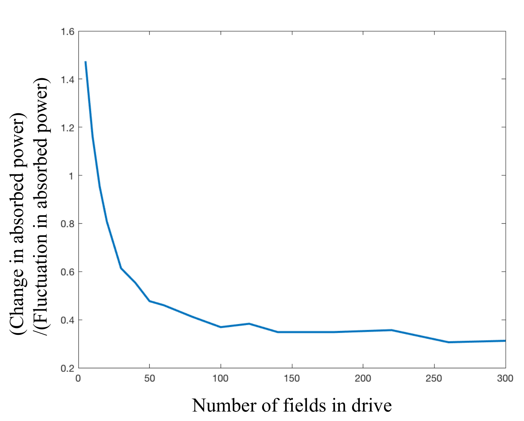
We sharpen this analysis. First, we divide the trial into time windows. During each time window, the field switches 10 times. (The 10 eliminates artificial noise and is not critical. Our qualitative results are robust with respect to changes in such details.) We measure the absorbed power at the end of each time window and at the start of the subsequent window. We define “the absorbed power jumps substantially” as “the absorbed power jumps, on average over trials, by much more than the noise (by much more than the absorbed power fluctuates across a trial)”:
| (D1) | ||||
Consider including only a few fields in the training drive, then growing the drive in later trials. The drive will tax the spin glass’s memory until exceeding the capacity. The LHS of (D1) will come to about equal the RHS.
Figure 10 illustrates with the spin glass. On the -axis is the number of fields in the training drive. On the -axis is the ratio of the left-hand side of Ineq. (D1) to the right-hand side (LHS/RHS). Where LHS/RHS , the spin glass reaches its capacity. This spin glass can remember fields, according to the absorbed power.
Appendix E Justification of use of machine learning
Deep learning is a powerful tool. Is it necessary for recovering our results? Could simpler algorithms detect and quantify many-body learning as sensitively? Comparable simpler algorithms tend not to, we find. Two competitors suggest themselves: single-layer linear autoencoders, related to PCA Bourland_88_Auto, and clustering algorithms. Alternatives include generalized linear models Bishop_06_Pattern and supervised linear autoencoders. These models, however, perform supervised learning. They receive more information than the VAE and so enjoy an unfair advantage. We analyze the two comparable competitors sequentially.
E 1 Comparison with single-layer linear autoencoder
The linear autoencoder is a single-layer NN. The input, , undergoes a linear transformation: . We compare, as follows, the linear autoencoder’s detection of field classification with the VAE’s detection: We trained the spin glass on a drive in each of 3,000-5,000 trials. Ninety percent of the trials were designated as NN-training data; and 10%, as NN-testing data. For each training trial, we identified the spin glass’s final configuration. On these configurations, each NN performed unsupervised learning. Each NN then received the configuration with which the spin glass ended a NN-testing trial. We inferred the field most likely to have produced this configuration, using MAP estimation. The fraction of trials in which the NN points to the correct field constitutes the NN’s score. On a three-field drive, the linear autoencoder scored 0.771, while the VAE scored 0.992. On a five-field drive, the linear autoencoder scored 0.3934, while the VAE scored 0.829. Hence the VAE picks up on more of the spin glass’s ability to classify fields.
E 2 Comparison with clustering algorithm
A popular, straightforward-to-apply algorithm is -means clustering Bishop_06_Pattern. refers to a parameter inputted into the algorithm, the number of clusters expected in the data. We inputted the number of drives imposed on the spin glass, in addition to inputting configurations. The VAE receives just configurations and so less information. We could level the playing field by automating the choice of , using the Bayesian information criterion (BIC) Bishop_06_Pattern. But clustering with the BIC-chosen would perform no better than clustering performed with the ideal , and the ideal clustering performs worse than the VAE.
The protocol run on the spin glass is described at the beginning of Sec. II B. Five thousand trials were performed. The configuration occupied by the spin glass at the end of each trial was collected. Splitting the data into testing and training data did not alter results significantly. Hence we fed all the configurations, with the number of drives, to the clustering algorithm. The algorithm partitioned the set of configurations into subsets. Each subset contained configurations likely to have resulted from the same drive.
Clustering algorithms are assessed with the Rand index, denoted by RI Rand_71_Objective. The Rand index differs from the MAP-estimation score (Sec. II A). How to compare the clustering algorithm with the VAE, therefore, is ambiguous. However, the Rand index quantifies the percentage of the algorithm’s classifications that are correct. Hence the Rand index and the MAP-estimation score have similar interpretations, despite their different definitions.
The clustering algorithm’s Rand index began at , at . RI rose during the first changes of the drive, then oscillated around 0.125. Figure 5 shows the VAE’s performance. The VAE’s score rose during the first changes of the drive, then oscillated around . Hence the VAE outperformed the clustering algorithm.
References
- (1) S. N. Coppersmith et al., Phys. Rev. Lett. 78, 3983 (1997).
- (2) M. L. Povinelli, S. N. Coppersmith, L. P. Kadanoff, S. R. Nagel, and S. C. Venkataramani, Phys. Rev. E 59, 4970 (1999).
- (3) N. C. Keim and S. R. Nagel, Phys. Rev. Lett. 107, 010603 (2011).
- (4) N. C. Keim, J. D. Paulsen, and S. R. Nagel, Phys. Rev. E 88, 032306 (2013).
- (5) J. D. Paulsen, N. C. Keim, and S. R. Nagel, Phys. Rev. Lett. 113, 068301 (2014).
- (6) S. Majumdar, L. C. Foucard, A. J. Levine, and M. L. Gardel, Soft Matter 14, 2052 (2018).
- (7) S. Mukherji, N. Kandula, A. K. Sood, and R. Ganapathy, Phys. Rev. Lett. 122, 158001 (2019).
- (8) W. Zhong, D. J. Schwab, and A. Murugan, Journal of Statistical Physics 167, 806 (2017).
- (9) N. C. Keim, J. D. Paulsen, Z. Zeravcic, S. Sastry, and S. R. Nagel, Rev. Mod. Phys. 91, 035002 (2019).
- (10) M. Nielsen, Neural Networks and Deep Learning (Determination Press, 2015).
- (11) I. Goodfellow, Y. Bengio, and A. Courville, Deep Learning (MIT Press, 2016), http://www.deeplearningbook.org.
- (12) A. Engel and C. P. L. V. d. Broeck, Statistical Mechanics of Learning (Cambridge University Press, New York, NY, USA, 2001).
- (13) A. A. Alemi and I. Fischer, arXiv:1807.04162 (2018).
- (14) Y. Bengio, A. Courville, and P. Vincent, arXiv:arXiv:1206.5538 (2012).
- (15) J. M. Gold and J. L. England, arXiv:1911.07216 (2019).
- (16) D. P. Kingma and M. Welling, arXiv:1312.6114 (2013).
- (17) D. Jimenez Rezende, S. Mohamed, and D. Wierstra, Stochastic Backpropagation and Approximate Inference in Deep Generative Models, in Proc. 31st Int. Conf. on Machine Learning, 2014.
- (18) C. Doersch, arXiv:1606.05908 (2016).
- (19) Online code, https://github.com/smarzen/Statistical-Physics, 2020.
- (20) C. M. Bishop, Pattern Recognition and Machine Learning (Springer, 2006).
- (21) H. Jaeger, Short-term memory in echo state networks, 2002.
- (22) C. D. Brown and H. T. Davis, Chemometrics and Intelligent Laboratory Systems 80, 24 (2006).
- (23) X. Cheng, J. H. McCoy, J. N. Israelachvili, and I. Cohen, Science 333, 1276 (2011), https://science.sciencemag.org/content/333/6047/1276.full.pdf.
- (24) T. Sanchez, D. T. N. Chen, S. J. DeCamp, M. Heymann, and Z. Dogic, Nature 491, 431 (2012).
- (25) J. Lonsdale et al., Nature Genetics 45, 580 (2013).
- (26) P. Vincent, H. Larochelle, Y. Bengio, and P.-A. Manzagol, Extracting and composing robust features with denoising autoencoders, in Proceedings of the 25th International Conference on Machine Learning, ICML ’08, pp. 1096–1103, New York, NY, USA, 2008, ACM.
- (27) D. J. Im, S. Ahn, R. Memisevic, and Y. Bengio, CoRR abs/1511.06406 (2015).
- (28) H. Bourlard and Y. Kamp, Biological Cybernetics 59, 291 (1988).
- (29) J. Miller, Physics Today (2019).
- (30) F. Heylighen, The Science of Self-Organization and Adaptivity (EOLSS Publishers Co Ltd, 2002), , in: L. D. Kiel, (ed.) Knowledge Management, Organizational Intelligence and Learning, and Complexity, in: The Encyclopedia of Life Support Systems ((EOLSS), (Eolss Publishers, Oxford). [http://www.eolss.net] Series editor: L. D. Kiel, (ed.).
- (31) T. Langen, R. Geiger, and J. Schmiedmayer, Annual Review of Condensed Matter Physics 6, 201 (2015), https://doi.org/10.1146/annurev-conmatphys-031214-014548.
- (32) N. Friis et al., Phys. Rev. X 8, 021012 (2018).
- (33) J. Smith et al., Nature Physics 12, 907 (2016).
- (34) G. Kucsko et al., Phys. Rev. Lett. 121, 023601 (2018).
- (35) D. A. Abanin, E. Altman, I. Bloch, and M. Serbyn, Rev. Mod. Phys. 91, 021001 (2019).
- (36) C. J. Turner, A. A. Michailidis, D. A. Abanin, M. Serbyn, and Z. Papic, Nature Physics 14, 745 (2018).
- (37) S. Still, D. A. Sivak, A. J. Bell, and G. E. Crooks, Phys. Rev. Lett. 109, 120604 (2012).
- (38) J. M. R. Parrondo, J. M. Horowitz, and T. Sagawa, Nature Physics 11, 131 (2015).
- (39) J. P. Crutchfield, arXiv:1710.06832 (2017).
- (40) A. Kolchinsky and D. H. Wolpert, Journal of Statistical Mechanics: Theory and Experiment 2017, 083202 (2017).
- (41) N. Tishby, F. C. Pereira, and W. Bialek, arXiv:physics/0004057 (2000).
- (42) N. Tishby, F. C. Pereira, and W. Biale, The information bottleneck method, in The 37th annual Allerton Conf. on Communication, Control, and Computing, pp. 368–377, 1999.
- (43) G. Carleo et al., Rev. Mod. Phys. 91, 045002 (2019).
- (44) T. Wu and M. Tegmark, Phys. Rev. E 100, 033311 (2019).
- (45) R. Iten, T. Metger, H. Wilming, L. del Rio, and R. Renner, Phys. Rev. Lett. 124, 010508 (2020).
- (46) D. Hafner, Building variational auto-encoders in tensorflow, Blog post, 2018.
- (47) W. M. Rand, Journal of the American Statistical Association 66, 846 (1971), https://www.tandfonline.com/doi/pdf/10.1080/01621459.1971.10482356.