The semi-classical approximation at high temperature revisited
Abstract
We revisit the semi-classical calculation of the size distribution of instantons at finite temperature in non-abelian gauge theories in four dimensions. The relevant functional determinants were first calculated in the seminal work of Gross, Pisarski and Yaffe and the results were used for a wide variety of applications including axions most recently. In this work we show that the uncertainty on the numerical evaluations and semi-analytical expressions are two orders of magnitude larger than claimed. As a result various quantities computed from the size distribution need to be reevaluated, for instance the resulting relative error on the topological susceptibility at arbitrarily high temperatures is about 5% for QCD and about 10% for Yang-Mills theory. With higher rank gauge groups this discrepancy is even higher. We also provide a simple semi-analytical formula for the size distribution with absolute error . In addition we also correct the over-all constant of the instanton size distribution in the scheme which was widely used incorrectly in the literature if non-trivial fermion content is present.
1 Introduction
This paper is concerned with the semi-classical study of gauge theories. At zero temperature or large space time volume the semi-classical picture is not reliable but at high temperature and finite spatial volume or small space time volume, the femto world Luscher:1981zf; Luscher:1982ma; Koller:1985mb; Koller:1987fq; vanBaal:1988va; vanBaal:1988qm, it is because the renormalized coupling runs with the relevant scale, or , and becomes small. In these regimes the path integral can accurately be computed as the saddle points associated with instantons and the perturbative fluctuations around them. At asymptotically large temperatures or asymptotically small space time volumes the higher charge sectors are suppressed relative to lower ones. If an observable only receives contributions from the non-zero sectors then the leading contribution is from the 1-instanton sector. For instance the topological susceptibility is such a quantity and the leading semi-classical result is fully determined by the size distribution of 1-instantons. This size distribution at high temperature is the object of study in the present paper.
There has been renewed interest in semi-classical results for the topological susceptibility in QCD at high temperature because of applications in axion physics; see Wantz:2009it and references therein, but also Pisarski:2019upw for unrelated recent developments. Basically, the topological susceptibility at high temperature can be used to constrain the amount of axions as dark matter components and its mass. In order to have results from first principles lattice calculations are ideal. Unfortunately the topological susceptibility decreases fast for hence a Monte-Carlo simulation will have a hard time achieving high precision because only very few configurations fall into the non-zero sectors. Even pure Yang-Mills theory is challenging in this respect Berkowitz:2015aua; Borsanyi:2015cka; Frison:2016vuc; Jahn:2018dke. Beyond pure Yang-Mills, results with dynamical fermions are also available Bonati:2015vqz; Petreczky:2016vrs; Borsanyi:2016ksw; Burger:2018fvb with full QCD Borsanyi:2016ksw reaching temperatures up to .
It is useful to compare the non-perturbative lattice results both in pure Yang-Mills and in full QCD with the semi-classical results. The relevant semi-classical expressions at finite temperature were first obtained in Pisarski:1980md; Gross:1980br. The instanton size distribution consists of two parts, the zero temperature expression and an extra factor responsible for the temperature dependence. In this work we report the correct zero temperature expression in the -scheme which was frequently used incorrectly once light fermions were included and secondly we also report that the factor responsible for the temperature dependence which was numerically evaluated in Gross:1980br has an uncertainty that is two orders of magnitude larger than claimed. In pure Yang-Mills theory only the latter issue is relevant and leads to an increase in the semi-classical prediction. Once fermions are included as in QCD, both issues become relevant and while the latter still leads to an increase, the former leads to a similar decrease.
The organization of the paper is as follows. In section 2 the basics of the semi-classical expansion as it relates to high temperatures is summarized, in section 3 the instanton size distribution is converted to the scheme and a frequent error is identified in the literature if non-trivial fermion content is present. The main result of the paper is contained in 4 where the temperature dependence of the instanton size distribution is calculated to high precision and in section 5 the results are applied to the topological susceptibility. Finally we end with some comments and conclusions in section 6.
2 Semi-classical expansion at high temperature
We will consider gauge theory with flavors of light fermions in the fundamental representation. The semi-classical approximation provides a consistent and reliable expansion of the path integral at fixed spatial volume and asymptotically high temperatures similarly to the situation in small 4-volume or femto world Luscher:1981zf; Luscher:1982ma; Koller:1985mb; Koller:1987fq; vanBaal:1988va; vanBaal:1988qm.
It is useful to consider the theory at non-zero angle and the partition function is then given by
| (1) |
where is the result of integrating over gauge fields with given topological charge . At high temperatures the sectors are suppressed relative to both exponentially in the inverse coupling as well as algebraically in the inverse temperature, similarly to the femto world. Hence we have the topological susceptibility as
| (2) |
where is the space-time volume and is the finite spatial box. Note that here we envisage a finite and large spatial volume and the limit . In this case all further terms in (2) are indeed negligible. For instance there is no need to invoke the dilute instanton gas approximation in order to obtain (2) at . The subject of the present paper is and our only objective is to study for so there is no reliance on the dilute instanton gas picture at all. In order to have a self contained presentation and clarify its relationship with the general semi-classical picture, we will nonetheless summarize the dilute instanton gas model in appendix A.
Now can be reliably calculated at asymptotically high temperatures as the contribution of the 1-instanton together with the perturbative fluctuations around it. The leading term is obtained by integration over the moduli space of 1-instanton solutions: where determines the position and the scale of the instanton. An integration over the arbitrary gauge orientation of the instanton is implied leading to an -dependent over-all factor. Integration over the position gives a space-time volume factor .
What we will be concerned with is the integration over the size or more precisely the size distribution ,
| (3) |
The size distribution at finite temperature Pisarski:1980md; Gross:1980br can be expressed by the analogous quantity at together with an explicitly temperature dependent factor ,
| (4) |
The zero temperature size distribution with light fermions at leading order is tHooft:1976snw; Bernard:1979qt
| (5) |
with the first coefficient of the -function and is a scheme-dependent constant. Its value will be detailed in the next section. The 2-loop expression for is actually available Morris:1984zi but for our purposes the leading order result is sufficient. Note that the constant in principle depends on given by the contribution of the non-zero mode fermion determinant Carlitz:1978yj; Novikov:1983gd; Kwon:2000kf; Dunne:2004sx but the massless limit can be taken for the asymptotically high temperature limit. It is assumed that the theory is renormalized at by introducing a renormalized coupling and renormalized masses at some renormalization scale in a chosen scheme. Once this is done is finite.
The presence of a finite temperature does not introduce any new divergences hence is also finite and by construction is zero at . For definiteness the renormalization scale can be chosen to be with some constant and the dependence on is indicative of higher order corrections. Since is dimensionless the only dependence is in fact through the variable . We have the result Brown:1978yj; Gross:1980br,
| (6) |
where the function ,
| (7) |
encodes the temperature dependence of the 1-loop determinant in the background of the instanton. Here determines the 1-instanton solution at finite temperature, the periodic Harrington-Shepard solution Harrington:1978ve, while is the corresponding function at zero temperature Belavin:1975fg,
| (8) | |||||
Both the first and second term in (7) are divergent separately and the second term, formally a constant, corresponding to zero temperature is subtracted in order to make finite and .
Summarizing the above, once is found the high temperature limit of and consequently that of the topological susceptibility is known.
The main object of study in the present paper is . The definition (7) can not be evaluated analytically. Numerically, the task is performing a 2 dimensional integral over and the careful subtraction of an infinite constant. This was first attempted in Gross:1980br and the numerical result was parametrized as,
| (9) |
with and and a quoted absolute numerical uncertainty of at most . Note that in Gross:1980br was denoted by but in order not to confuse it with Euler’s constant later we will label it by . Formula (9) was then used in all subsequent applications Berkowitz:2015aua; Borsanyi:2015cka; Kitano:2015fla; Frison:2016vuc where the topological susceptibility was studied at high temperatures and compared with the semi-classical results.
In the present paper we show that the actual numerical accuracy of (9) is two orders of magnitude larger than claimed in Gross:1980br at around leading to about a 5% mismatch for the topological susceptibility in QCD or 10% mismatch for pure Yang-Mills. For higher rank gauge groups the mismatch is even higher. Any absolute error on needs to be scaled by for the absolute accuracy of and this scaled absolute accuracy becomes the relative accuracy of the topological susceptibility.
Before calculating accurately in section 4 we make a comment in the next section on the constant appearing in (5). It turns out its flavor number dependence in the scheme was widely used incorrectly in the literature, especially recently in axion mass estimates as well as comparisons with lattice results.
3 Scheme dependence - conversion to
Historically, there has been quite a bit of confusion about the constant in (5). The topological susceptibility is of course a finite RG invariant quantity but its perturbative expansion in terms of a scheme dependent running coupling involve the scheme dependent constant . In the original paper tHooft:1976snw a Pauli-Villars regulator was used for which was extended to still with a Pauli-Villars regulator in Bernard:1979qt. The Pauli-Villars results in tHooft:1976snw were correct except for some trivial mistakes corrected later in an erratum, but the conversion to the MS scheme was incorrect. The correct conversion factor was later found in Hasenfratz:1980kn and confirmed in tHooft:1986ooh. It is possible to work directly within the MS scheme lending further support to the correct conversion factor Luscher:1982wf. The conversion between various schemes is via the -parameter ratios, more precisely the constants in two different schemes are related by
| (10) |
For definiteness we record the ones relevant for us below Bardeen:1978yd; Hasenfratz:1980kn,
| (11) |
Note that wrong -parameter ratios were published for instance in Weisz:1980pu as well as Dashen:1980vm. The scheme is one of the most frequently used schemes and the constant can trivially be obtained from either the Pauli-Villars or the MS scheme. The result is
| (12) | |||||
with the derivative of the Riemann -function . Even though there is now consensus on the pure Yang-Mills case, the flavor coefficient in was frequently quoted Ringwald:1998ek as in the notation of tHooft:1976snw and subsequently this value was used in applications Berkowitz:2015aua; Borsanyi:2015cka; Frison:2016vuc. 11 1 In an earlier work was reported Moch:1996bs based on Balitsky:1992vs which is also incorrect. However equals which is the relevant result within the Pauli-Villars scheme, the one obtained in tHooft:1976snw. It appears that only the coefficient was converted to and the flavor coefficient was not although of course depends on . The mismatch in is precisely which should be included using (10) and (11). Here comes from the -function and from the ratio of the -parameters.
4 Calculation of
It is seemingly a relatively straightforward task to evaluate (7). However analytical evaluation is apparently impossible and numerical integration is tricky primarily because of the subtraction of the infinite constant and a need for high arithmetic precision.
The 2 dimensional integral responsible for the -dependence is over where is a periodic variable with period . First, we will perform this integral over analytically and only the second integral over will be left numerically. Let us rescale both and by so that they become dimensionless and periodic with period . Then we have
| (13) | |||||
where prime denotes differentiation with respect to . Now the -integral can be done analytically for instance via the residue theorem and we obtain,
| (14) | |||||
where the and derivatives should be taken at fix and in the end are all simple functions of .
In a similar fashion let us integrate out in the second term of (7) containing responsible for subtracting an infinite constant. In this term can be made dimensionless by rescaling by and we obtain,
Now we have both terms in (7) in terms of a dimensionless and arrive at,
| (15) |
The integrals with or are separately divergent and the divergence comes from the origin. For finite and fixed they both behave as for hence the difference is finite. For both terms are integrable separately. More specifically we have,
Hence (15) defines a convergent integral for . Numerical evaluation is straightforward although high arithmetic precision is required because of large cancellations. First, the cancellation between and in (15) needs to be resolved and also the evaluation of itself via (14) involve large cancellations especially for small . As we will see the discrepancy between our result and Gross:1980br is precisely here in the small region. We have found that keeping significant digits is nonetheless sufficient.
In order to have as much analytic control as possible it is useful to derive the small and large asymptotics which will be used to check the numerical results.
4.1 Small and large asymptotics
It is relatively straightforward to obtain the asymptotics. The simplest is to change the integration variable in (15), expand the integrand in and perform the -integral. The first 3 terms are,
| (20) |
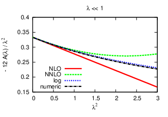
where the terms may include fractional powers and/or logarithms and it turns out that the log on the right hand side has the same first 3 Taylor coefficients as the ones obtained from the integral. These 3 terms will be referred to as LO, NLO, NNLO in the following.
The regime is more difficult to obtain. Starting with the original expression (15) one may split the integral to two intervals, and with some fixed . In the limit the first term is finite whereas the second term is logarithmically divergent.
More specifically, the first term can be straightforwardly expanded in leading to a constant and subleading expressions. In the integral all exponentials may be dropped, the integration over can then be performed and the result can be expanded in . Finally in the sum of the two integrals, order by order in , can be taken in order to justify the dropping of all exponentials. This procedure leads to,
| (21) |
The divergent piece is originating from the second integral in the above split. The 4 terms above will be referred to as LO, NLO, NNLO and N3LO in the following, similarly to the small expansion.
Clearly, the parametrization (9) satisfies the small expansion (20). However, even though the small expansion of the second term of (9) is its coefficient is rather large and distorts the small behavior. Quite remarkably the NLO large expansion (4.1) matches (9) since the constant term in (9) is which agrees with to 6 significant digits. However the NNLO and N3LO terms of the large expansions do not match (9) but for the application to the topological susceptibility this matters much less than the mismatch at .
4.2 Numerical results
After making sure the arithmetic precision is high enough it is straightforward to calculate numerically using (15). First, numerical integration is done on the interval with either the trapezoid or Simpson’s rule with step size . The difference between the two schemes is at most which is the estimated accuracy. The remaining integral on can be approximated by dropping all exponentials in the integrand and performing the integral analytically. This second piece is then added to the numerical integral on the finite interval and amounts to at most . We have checked that the exact integrand at agrees with the one where the exponentials are dropped to either or the added term is at most . The procedure is then reliable in absolute precision to at least .
The final result is shown in figure 1. The numerical result is compared with the increasing orders of both the small and large expansions in figure 2 showing increasing agreement order by order in both regimes as expected.
Let us now compare with Gross:1980br. We show the difference between the parametrization (9) and the numerical result in the left panel of figure 3. Clearly, the difference is well outside the claimed absolute precision of . Note that any absolute error on will turn into a relative error on the size distribution. Unfortunately, the differences are largest for which is precisely the region which contributes the most to the topological susceptibility through the integration over the instanton sizes.
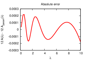
We have found that the following is a convenient parametrization with at most deviation from the numerical over the full range ,
| (22) | |||||
The difference with respect to the numerically evaluated is shown in the right panel of figure 3.
5 Topological susceptibility at high temperature
Once a reliable result for is obtained the topological susceptibility at asymptotically high temperatures can be calculated using (3) - (6). Here we are interested in studying the discrepancy between using (9) and our result (22) for the topological susceptibility for various gauge groups and fermion content. It is a simple exercise to compute the integrals over the instanton size and it turns out that there is an approximately 10% discrepancy between them for pure Yang-Mills and about 7%, 6% and 4% for 2, 3 and 4 light flavors, respectively, with the correct results being larger by these amounts. For fixed the largest relative difference is always at and for increasing the discrepancy grows. For instance with we have about 22% while with it is about 40% which is quite sizable. The reason for this exploding discrepancy is that in the large- limit the size distribution is more and more peaked around which unfortunately is approximately where the discrepancy between our result and Gross:1980br is largest in absolute terms, see left panel of figure 3, and any absolute discrepancy is scaled up by . The large absolute discrepancy is translated into a large relative discrepancy for the topological susceptibility. Since only instantons of the critical size contribute in the large- limit, a straightforward explicit expression can in fact be obtained for the topological susceptibility.
Recently there has been renewed interest in the non-perturbative determination of the topological susceptibility in lattice calculations DelDebbio:2004vxo; Berkowitz:2015aua; Borsanyi:2015cka; Kitano:2015fla; Bonati:2015vqz; Frison:2016vuc; Petreczky:2016vrs; Borsanyi:2016ksw; Dine:2017swf; Burger:2018fvb; Jahn:2018dke motivated mainly by axion physics. Even the pure Yang-Mills case is challenging and obtaining high precision results at high enough temperatures is difficult. It is nevertheless clear Borsanyi:2015cka; Jahn:2018dke that at the temperature is not high enough for the semi-classical topological susceptibility to agree with the non-perturbative lattice result, however at the two already only deviate Jahn:2018dke within . The lattice result Jahn:2018dke extrapolated to the continuum is , whereas the semi-classical one is where the 2-loop result for the susceptibility itself Morris:1984zi and 5-loop running Baikov:2016tgj; Herzog:2017ohr for the coupling was used (however 3-loop or 4-loop running for the coupling gives identical results). The first error estimate includes the residual dependence on the scale and the second (dominant) one originates from the uncertainty of which was also obtained in lattice calculations Borsanyi:2012ve. Note that without lattice input it is only possible to obtain the semi-classical susceptibility in units with the temperature also measured in , however the lattice results for the susceptibility are in units so the uncertainty related to is unavoidable. The resulting uncertainty is rather large because the power of enters the semi-classical susceptibility.
In QCD the situation Borsanyi:2016ksw is similar in that the semi-classical susceptibility is in units and with 4 flavors ; the uncertainty is about 5% Tanabashi:2018oca. This uncertainty is amplified by the even higher factor in the logarithm of the susceptibility, leading to the semi-classical result at where again the inherent uncertainty of the semi-classical result is negligible compared to the one associated with the uncertainty of the scale. The corresponding flavor lattice result extrapolated to the continuum is hence the deviation between the two is about ; for higher temperature the deviation is decreasing Borsanyi:2016ksw. The semi-classical result is consistently below the lattice result, similarly to pure Yang-Mills, and it is most likely that further perturbative corrections to the 2-loop semi-classical topological susceptibility are responsible for the current deviation at the relatively high temperature reachable today by lattice calculations. Note that in QCD the two issues reported in this paper (more accurate and correct ) nearly cancel each other in the final result.
6 Conclusions
In this paper we have studied the instanton size distribution in gauge theories with light fermions semi-classically. At large but finite spatial volume and asymptotically high temperatures the contribution of the 1-instanton sector is the exact result, there is no need to invoke the dilute instanton gas model. We were motivated by the recent interest in the semi-classical calculation of the topological susceptibility at high temperature which in turn was motivated by axion physics.
It turned out that there were two issues in previous semi-classical calculations which led to incorrect results. One, even at zero temperature the over-all constant of the instanton size distribution was not correctly converted to when and second, the numerically evaluated 1-loop determinant in the instanton background was two orders of magnitude less precise than originally thought. We have managed to evaluate these determinants to high precision with an absolute uncertainty of at most by doing the periodic integral over the temperature analytically leaving only a one dimensional integral numerically which could be handled by standard methods. Although the discrepancy with previous work is not large the integration over the instanton size is peaked at around the same point where the discrepancy is largest. Any discrepancy in absolute terms is then converted to a relative discrepancy for the topological susceptibility which can be 10% for or larger for higher gauge groups.
Once correct semi-classical expressions are obtained a meaningful comparison with the lattice results can be carried out however the uncertainty of the scale needs to be taken into account. Taking everything into account in pure Yang-Mills the semi-classical and lattice results already at are within Jahn:2018dke and with flavor QCD at the deviation is below Borsanyi:2016ksw. The remaining deviation can surely be reduced by simply considering higher temperatures which is however quite demanding on the lattice or by calculating further perturbative corrections to the semi-classical result.
Acknowledgments
We are grateful to Sandor Katz, Tamas Kovacs, Andreas Ringwald and Kalman Szabo for insightful discussions and helpful comments on the manuscript. The work of DN was supported by NKFIH under the grant KKP-126769.
Appendix A The dilute instanton gas model
As emphasized throughout the paper the asymptotically high temperature limit at fixed spatial volume as well as the small space time volume limit are accessible to semi-classical calculations. In these two regimes the path integral can be computed by the contribution of instantons and the perturbative fluctuations around them. If a given accuracy is required, only a finite number of topological sectors need to be considered. If only the leading behavior is required then one needs to include only the first sector which gives a non-zero result. Apart from being at high temperature or small space time volume, no further assumptions are needed and the results can be made arbitrarily precise by increasing the perturbative order at fixed sector and by including more and more sectors. In this sense the semi-classical results are exact in these two regimes.
The dilute instanton gas model on the other hand is an uncontrolled approximation. The assumption is the presence of some positively and negatively charged but otherwise indistinguishable and independent objects with a constant density. A priori there does not need to be any reference to weak coupling or semi-classical objects. Then the contribution of all sectors will be fixed in terms of a single variable which can be chosen as and we have,
| (23) |
which immediately leads to,
| (24) |
where is the modified Bessel-function of the first kind. The probability to find a gauge field with charge is then,
| (25) |
Hence the single parameter determines all -dependence and the full topological charge distribution. Unsurprisingly we have,
| (26) |
i.e. the single parameter is indeed the topological susceptibility.
We emphasize again that a priori there does not need to be any reference to weak coupling or semi-classical objects at all in order for (23) - (25) to hold with some parameter . Perhaps it would be more accurate to call these set of assumptions the ideal gas model rather than the dilute instanton gas model in order to make this distinction clear. This is because the following two questions are independent at a given temperature: (A) whether the semi-classical expansion at fixed order is accurate or not and (B) whether the topological charge distribution and the full -dependence follows (23) - (25) with a single parameter or not. As to question (A) we know that the semi-classical expansion is reliable at finite spatial volume and asymptotically high temperatures without any further assumptions. At asymptotically high temperatures (B) is also true with given by the semi-classical result (2) however at asymptotically high temperatures all the additional assumptions (23) - (25) are not necessary, the semi-classical picture alone is sufficient to calculate anything. Question (B) becomes a non-trivial proposition at finite temperature where perhaps it does hold, although there is no a priori reason for it, with some parameter which is however different from the semi-classical result (2). This is precisely what appears to be the case based on detailed lattice calculations in the pure Yang-Mills case Bonati:2013tt; Kovacs:2017pox; Vig:2019wei. Immediately above the topological charge distribution seems to follow (25) but with a which is non-perturbative and does not agree with the semi-classical formula. This comparison is what we would call testing the ideal gas model. It would be very interesting to extend these results to full QCD; for some recent results see Bonati:2018blm.
References
- (1) M. Luscher, Nucl. Phys. B 205, 483 (1982).
- (2) M. Luscher, Nucl. Phys. B 219, 233 (1983).
- (3) J. Koller and P. van Baal, Nucl. Phys. B 273, 387 (1986).
- (4) J. Koller and P. van Baal, Nucl. Phys. B 302, 1 (1988).
- (5) P. van Baal, Nucl. Phys. B 307, 274 (1988) Erratum: [Nucl. Phys. B 312, 752 (1989)].
- (6) P. van Baal, Acta Phys. Polon. B 20, 295 (1989).
- (7) O. Wantz and E. P. S. Shellard, Phys. Rev. D 82, 123508 (2010) [arXiv:0910.1066 [astro-ph.CO]].
- (8) R. D. Pisarski and F. Rennecke, arXiv:1910.14052 [hep-ph].
- (9) E. Berkowitz et al., Phys. Rev. D 92, no. 3, 034507 (2015) [arXiv:1505.07455 [hep-ph]].
- (10) S. Borsanyi et al., Phys. Lett. B 752, 175 (2016) [arXiv:1508.06917 [hep-lat]].
- (11) J. Frison et al., JHEP 1609, 021 (2016) [arXiv:1606.07175 [hep-lat]].
- (12) P. T. Jahn et al., Phys. Rev. D 98, no. 5, 054512 (2018) [arXiv:1806.01162 [hep-lat]].
- (13) C. Bonati et al., JHEP 1603, 155 (2016) [arXiv:1512.06746 [hep-lat]].
- (14) P. Petreczky, H. P. Schadler and S. Sharma, Phys. Lett. B 762, 498 (2016) [arXiv:1606.03145 [hep-lat]].
- (15) S. Borsanyi et al., Nature 539, no. 7627, 69 (2016) [arXiv:1606.07494 [hep-lat]].
- (16) M. Dine, P. Draper, L. Stephenson-Haskins and D. Xu, Phys. Rev. D 96, no. 9, 095001 (2017) [arXiv:1705.00676 [hep-ph]].
- (17) F. Burger et al., Phys. Rev. D 98, no. 9, 094501 (2018) [arXiv:1805.06001 [hep-lat]].
- (18) R. D. Pisarski and L. G. Yaffe, Phys. Lett. 97B (1980) 110.
- (19) D. J. Gross, R. D. Pisarski and L. G. Yaffe, Rev. Mod. Phys. 53, 43 (1981).
- (20) G. ’t Hooft, Phys. Rev. D 14, 3432 (1976) Erratum: [Phys. Rev. D 18, 2199 (1978)].
- (21) C. W. Bernard, Phys. Rev. D 19, 3013 (1979).
- (22) T. R. Morris, D. A. Ross and C. T. Sachrajda, Nucl. Phys. B 255, 115 (1985).
- (23) R. D. Carlitz and D. B. Creamer, Annals Phys. 118, 429 (1979).
- (24) V. A. Novikov, M. A. Shifman, A. I. Vainshtein and V. I. Zakharov, Fortsch. Phys. 32, 585 (1984).
- (25) O. K. Kwon, C. k. Lee and H. Min, Phys. Rev. D 62, 114022 (2000) [hep-ph/0008028].
- (26) G. V. Dunne, J. Hur, C. Lee and H. Min, Phys. Rev. Lett. 94, 072001 (2005) [hep-th/0410190].
- (27) L. S. Brown and D. B. Creamer, Phys. Rev. D 18, 3695 (1978).
- (28) B. J. Harrington and H. K. Shepard, Phys. Rev. D 17, 2122 (1978).
- (29) A. A. Belavin, A. M. Polyakov, A. S. Schwartz and Y. S. Tyupkin, Phys. Lett. 59B, 85 (1975).
- (30) R. Kitano and N. Yamada, JHEP 1510, 136 (2015) [arXiv:1506.00370 [hep-ph]].
- (31) A. Hasenfratz and P. Hasenfratz, Phys. Lett. 93B, 165 (1980).
- (32) G. ’t Hooft, Phys. Rept. 142, 357 (1986).
- (33) M. Luscher, Annals Phys. 142, 359 (1982).
- (34) W. A. Bardeen, A. J. Buras, D. W. Duke and T. Muta, Phys. Rev. D 18, 3998 (1978).
- (35) P. Weisz, Phys. Lett. 100B, 331 (1981).
- (36) R. F. Dashen and D. J. Gross, Phys. Rev. D 23, 2340 (1981).
- (37) A. Ringwald and F. Schrempp, Phys. Lett. B 438, 217 (1998) [hep-ph/9806528].
- (38) S. Moch, A. Ringwald and F. Schrempp, Nucl. Phys. B 507, 134 (1997) [hep-ph/9609445].
- (39) I. I. Balitsky and V. M. Braun, Phys. Rev. D 47, 1879 (1993).
- (40) L. Del Debbio, H. Panagopoulos and E. Vicari, JHEP 0409, 028 (2004) [hep-th/0407068].
- (41) P. A. Baikov, K. G. Chetyrkin and J. H. Kühn, Phys. Rev. Lett. 118, no. 8, 082002 (2017) [arXiv:1606.08659 [hep-ph]].
- (42) F. Herzog, B. Ruijl, T. Ueda, J. A. M. Vermaseren and A. Vogt, JHEP 1702, 090 (2017) [arXiv:1701.01404 [hep-ph]].
- (43) S. Borsanyi, G. Endrodi, Z. Fodor, S. D. Katz and K. K. Szabo, JHEP 1207, 056 (2012) [arXiv:1204.6184 [hep-lat]].
- (44) M. Tanabashi et al. [Particle Data Group], Phys. Rev. D 98, no. 3, 030001 (2018). doi:10.1103/PhysRevD.98.030001
- (45) C. Bonati, M. D’Elia, H. Panagopoulos and E. Vicari, Phys. Rev. Lett. 110, no. 25, 252003 (2013) [arXiv:1301.7640 [hep-lat]].
- (46) T. G. Kovacs, EPJ Web Conf. 175, 01013 (2018) [arXiv:1711.03911 [hep-lat]].
- (47) R. A. Vig and T. G. Kovacs, arXiv:1911.10086 [hep-lat].
- (48) C. Bonati, M. D’Elia, G. Martinelli, F. Negro, F. Sanfilippo and A. Todaro, JHEP 1811, 170 (2018) [arXiv:1807.07954 [hep-lat]].