microbatchGAN: Stimulating Diversity with Multi-Adversarial Discrimination

Gonçalo Mordido Haojin Yang Christoph Meinel Affiliation: Hasso Plattner Institute Email: goncalo.mordido@hpi.de

Abstract

We propose to tackle the mode collapse problem in generative adversarial networks (GANs) by using multiple discriminators and assigning a different portion of each minibatch, called microbatch, to each discriminator. We gradually change each discriminator’s task from distinguishing between real and fake samples to discriminating samples coming from inside or outside its assigned microbatch by using a diversity parameter $\alpha$ . The generator is then forced to promote variety in each minibatch to make the microbatch discrimination harder to achieve by each discriminator. Thus, all models in our framework benefit from having variety in the generated set to reduce their respective losses. We show evidence that our solution promotes sample diversity since early training stages on multiple datasets.

1 Introduction

Generative adversarial networks [12], or GANs, consist of a framework describing the interaction between two different models - one generator (G) and one discriminator (D) - that are trained together. While $G$ tries to learn the real data distribution by generating realistic looking samples that are able to fool $D$ , $D$ tries to do a better job at distinguishing between real and the fake samples produced by $G$ . Although showing very promising results across various domains [11, 14, 41, 40, 8] , GANs have also been continually associated with instability in training, more specifically mode collapse [16, 1, 25, 5, 2]. This behavior is observed when $G$ is able to fool $D$ by only generating samples from the same data mode, leading to very similar looking generated samples. This suggests that $G$ did not succeed in learning the full data distribution but, instead, only a small part of it. This is the main problem we are trying to solve with this work.

The proposed solution is to use multiple discriminators and assign each $D$ a different portion of the real and fake minibatches, i.e., microbatch. Then, we update each $D$ ’s task to discriminate between samples coming from its assigned fake microbatch and samples from the microbatches assigned to the other discriminators, together with the real samples. We call this microbatch discrimination. Throughout training, we gradually change from the originally proposed real and fake discrimination by [12] to the introduced microbatch discrimination by the use of an additional diversity parameter $\alpha$ that ultimately controls the diversity in the overall minibatch.

The main idea of this work is to force $G$ to reduce its loss by inducing variety in the generated set, complicating each $D$ ’s task on separating the samples in its microbatch from the rest. Even though only producing very similar images would also complicate the desired discrimination, it would not benefit any of the models. This is due to the attribution of distinct probabilities by each $D$ to samples from and outside its microbatch being required to minimize $G$ and $D$ ’s losses. Hence, all models in the proposed framework, called microbatchGAN, benefit directly from diversity in the generated set.

Our main contributions can be stated as follows: (i) proposal of a novel multi-adversarial GANs framework (Section 3) that mitigates the inherent mode collapse problem in GANs; (ii) empirical evidence on multiple datasets showing the success of our approach in promoting sample variety since early stages of training (Section 4) (iii) Competitiveness against other previously proposed methods on multiple datasets and evaluation metrics (Section 5).

1.1 Related Work

Previous works have optimized GANs training by changing the overall models’ objectives, either by using discrepancy measurements [20, 35] or different divergence functions [31, 36] to approximate the real data distribution. Moreover, [42, 4, 37] proposed to use energy-driven objective functions to encourage sample variety, [28] tried to match the mean and covariance of the real data, and [26] used an unrolled optimization of $D$ to train $G$ . [5, 39, 38, 4] penalized missing modes by using an extra autoenconder in the framework. [33] performed minibatch discrimination by forcing $D$ to condition its output on the similarity between the samples in the minibatch. [34] increased $D$ ’s robustness by maximizing the mutual information between inputs and corresponding labels, while [21] forced $D$ to make decisions over multiple samples of the same class, instead of independently.

Regarding using multiple discriminators, [29] extended the framework to several discriminators with each focusing in a low-dimensional projection of the data, set a priori. [10] proposed GMAN, consisting of an ensemble of discriminators that could be accessed by the single generator according to different levels of difficulty. [30] introduced D2GAN, introducing a single generator dual discriminator architecture where one discriminator rewards samples coming from the true data distribution whilst the other rewards samples coming from the generator, forcing the generator to continuously change its output. [27] proposed Dropout-GAN, applying adversarial dropout by omitting the feedback of a given $D$ at the end of each batch.

2 Generative Adversarial Networks

The original GANs framework [12] consists of two models: a generator ( $G$ ) and a discriminator ( $D$ ). Both models are assigned different tasks: whilst $G$ tries to capture the real data distribution $p_{r}$ , $D$ learns how to distinguish real from fake samples. $G$ maps a noise vector $z$ , retrieved from a noise distribution $p_{z}$ , to a realistic looking sample belonging to the data space. $D$ maps a sample to a probability $p$ , representing the likeliness of that given sample coming from $p_{r}$ rather than from $p_{g}$ . The two models are trained together and play the following minimax game:

\begin{split}\min_{G}\max_{D}V(D,G)=\\ \E_{x\sim p_{r}(x)}[\log D(x)]+\E_{z\sim p_{z}(z)}[\log(1-D(G(z)))],\end{split}

(1)

where $D$ maximizes the probability of assigning samples to the correct distribution and $G$ minimizes the probability of its samples being considered from the fake data distribution.

Alternatively, one can also train $G$ to maximize the probability of its output being considered from the real data distribution, i.e., $\log D(G(z))$ . Even though this changes the type of the game, by being no longer minimax, it avoids the saturation of the gradient signals at the beginning of training [12], where $G$ only receives continuously negative feedback, making training more stable in practice. However, since we employ multiple discriminators in the proposed framework, it is less likely that $G$ does not receive any positive feedback from the whole adversarial ensemble [10]. Therefore, we make use of the original value function in this work.

3 microbatchGAN

In this work, we propose a novel generative multi-adversarial framework named microbatchGAN, where we start by splitting each minibatch into several microbatches and assigning a unique one to each $D$ . The key aspect of this work is the usage of microbatch discrimination, where we change the original discrimination task of distinguishing between real and fake samples, as proposed in [12], to each $D$ distinguishing between samples coming or not from its fake microbatch. This change is performed in a gradual fashion, using an additional diversity parameter $\alpha$ . Thus, each $D$ ’s output gradually changes from the probability of a given sample being real to the probability of a given sample not belonging to its fake microbatch. Moreover, since each $D$ is trained with different fake and real samples, we encourage them to focus on different data properties. Figure 1 illustrates the proposed framework.

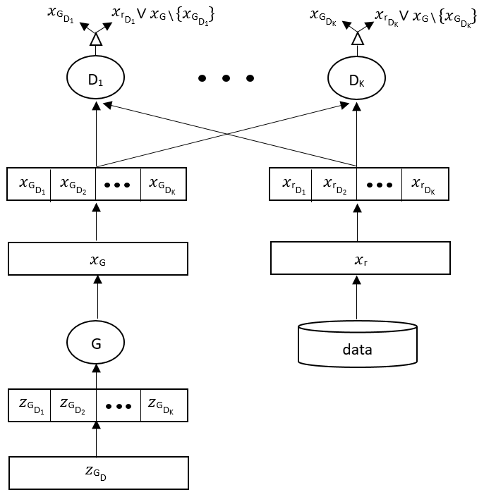
Refer to caption — Figure 1: microbatchGAN framework assuming a positive diversity parameter $\alpha$ . Each discriminator $D_{k}$ is assigned a different microbatch $x_{G_{D_{k}}}$ , where it discriminates between samples coming from inside its microbatch and samples coming from the microbatches assigned to the rest of the discriminators ( $x_{G}\setminus x_{G_{D_{k}}}$ ) together the real samples $x_{r_{D_{k}}}$ .

The proposed microbatch-level discrimination task leads to $G$ making such discrimination harder for each $D$ to lower its loss. Hence, $G$ is forced to induce variety on the overall minibatch, making it a substantially harder task for each $D$ to be able to separate its subset of fake samples in the diverse minibatch. Note that producing very similar samples across the whole minibatch would also make such discrimination difficult by making the whole minibatch the same. However, $G$ also benefits from each $D$ assigning distinct probabilities to samples from inside and outside its designed microbatch to lower its loss, making the generation of different samples in the minibatch a necessary requirement to obtain different outputs from $D$ . Hence, all models in our framework benefit directly from sample variety in the generated set.

In the microbatchGAN scenario with a positive diversity parameter $\alpha$ , each $D$ assigns low probabilities to fake samples from its microbatch and high probabilities to fake samples from the rest of the microbatches as well as samples from the real data distribution. Hence, fake samples in the rest of the minibatch, i.e., not coming from its assigned microbatch, shall be given distinct output probabilities by each $D$ . On the other hand, $G$ minimizes the probability given by each $D$ to the samples outside its microbatch and maximizes the probability given to the fake samples assigned to that specific $D$ . The value function of our minimax game is as follows:

\begin{split}\min_{G}\max_{\big\{D_{k}\big\}}\sum_{k=1}^{K}V(D_{k},G)=\sum_{k=1}^{K}\E_{x\sim p_{r_{D_{k}}}(x)}[\log D_{k}(x)]\\ +\E_{z\sim p_{z_{G_{D_{k}}}}(z)}[\log(1-D_{k}(G(z)))]\\ +\alpha\times\E_{z^{\prime}\sim p_{z_{G_{D}}\setminus\small\{z_{G_{D_{k}}}\small\}}(z^{\prime})}[\log D_{k}(G(z^{\prime}))],\end{split}

(2)

where K represents the number of total discriminators in the set. $p_{r_{D_{k}}}$ represents real samples from $D_{k}$ ’s real microbatch, $p_{z_{G_{D_{k}}}}$ indicates fake samples from $D_{k}$ ’s fake microbatch, and $p_{z_{G_{D}}\setminus\small\{z_{G_{D_{k}}}\small\}}$ relates to the rest of the fake samples in the minibatch but not in $p_{z_{G_{D_{k}}}}$ . $\alpha$ represents the diversity parameter responsible for penalizing the incorrect discrimination of fake samples coming from $p_{z_{G_{D}}\setminus\small\{z_{G_{D_{k}}}\small\}}$ by each $D_{k}$ . Note that $\alpha$ = 0 would represent the original GANs objective for each $D$ in the set. The training procedure of microbatchGAN is presented in Algorithm 1.

Algorithm 1 microbatchGAN.

Input:

K

number of discriminators,

\alpha

diversity parameter,

B

minibatch size

Initialize:

m\leftarrow\frac{B}{K}

for number of training iterations do

• Sample minibatch

z_{i}

i=1\ldots B

z_{i}\sim p_{g}(z)

• Sample minibatch

x_{i}

i=1\ldots B

x_{i}\sim p_{r}(x)

for

k=1

k=K

• Sample microbatch

z_{k_{j}}

j=1\ldots m

z_{k_{j}}=z_{(k-1)\times m+1:k\times m}

• Sample microbatch

x_{k_{j}}

j=1\ldots m

x_{k_{j}}=x_{(k-1)\times m+1:k\times m}

• Sample microbatch

z^{\prime}_{k_{j}}

j=1\ldots m

z^{\prime}_{k_{j}}\subset z_{i}\setminus\small\{z_{k_{j}}\small\}

• Update

D_{k}

by ascending its stochastic gradient:

\nabla_{\theta_{D_{k}}}\frac{1}{m}\sum_{j=1}^{m}[\log D_{k}(x_{k_{j}})+\log(1-D_{k}(G(z_{k_{j}})))

+\alpha\times\log D_{k}(G(z^{\prime}_{k_{j}}))]

end for

• Update

G

by descending its stochastic gradient:

\nabla_{\theta_{G}}\sum_{k=1}^{K}\big[\frac{1}{m}\sum_{j=1}^{m}[\log(1-D_{k}(G(z_{k_{j}})))

+\alpha\times\log D_{k}(G(z^{\prime}_{k_{j}}))]\big]

end for

3.1 Theoretical Discussion

To better understand how our approach differs from the original GANs in promoting variety in the generated set, we study a simplified version of the minimax game where we freeze each $D_{k}$ and train $G$ until convergence. In the most extreme case, we say that we have mode collapse when:

\text{For all }z^{\prime}\sim p_{g}(z),G(z^{\prime})=x

(3)

Theorem 1.

In original GANs, mode collapse fully minimizes $G$ ’s loss when we train $G$ exhaustively without updating $D$ .

Proof.

The optimal $x^{\ast}$ is the one that maximizes $D$ ’s output, where: $x^{\ast}=\underset{x}{\text{argmax}}D(x)$ . Thus, assuming $G$ would eventually learn how to produce $x^{\ast}$ , mode collapse on $x^{\ast}$ would fully minimize its loss, making $x^{\ast}$ independent of $z$ . ∎

Theorem 2.

In microbatchGAN, assuming $\alpha>0$ , $x\sim p_{g}$ must be dependent of $z$ for $G$ to fully minimize its loss, mitigating mode collapse when we train $G$ exhaustively without updating any $D_{k}$ .

Proof.

From Eq. 2, the value function between $G$ and each $D_{k}$ can be expressed as

\begin{split}V(D_{k},G)=\E_{x\sim p_{r}}[\log D_{k}(x)]+\E_{x^{\prime}\sim p_{g}}[\log(1-D_{k}(x^{\prime}))]\\ +\alpha\times\E_{x^{\prime\prime}\sim p_{g}}[\log D_{k}(x^{\prime\prime})].\end{split}

(4)

To fully minimize its loss in relation to $D_{k}$ , $G$ must find

x^{\prime}=\underset{x}{\text{argmax}}D_{k}(x)\text{ and }x^{\prime\prime}=\underset{x}{\text{argmin}}D_{k}(x),

(5)

which implies

D_{k}(x^{\prime})\neq D_{k}(x^{\prime\prime})\implies x^{\prime}\neq x^{\prime\prime}.

(6)

Thus, generating different outputs for different $z$ is a requirement to fully minimize $G$ ’s loss regarding each $D_{k}$ . Since we sum all $V(D_{k},G)$ to calculate $G$ ’s final loss, this also applies to overall adversarial set, concluding the proof.

∎

3.2 Diversity Parameter $\alpha$

We control the weight of the microbatch discrimination in the models’ losses by introducing an additional diversity parameter $\alpha$ . Lower $\alpha$ values lead to $G$ significantly lowering its loss by generating realistic looking samples on each microbatch without taking much consideration on the variety of the overall minibatch. On the other hand, higher $\alpha$ values induce a stronger effect on $G$ ’s loss if each $D$ is able to discriminate between samples inside and outside its microbatch. However, high values of $\alpha$ might compromise the realistic properties of the produced samples, since too much weight is given to the last part of Eq. 2, being sufficient to effectively minimize $G$ ’s loss. Thus, using $\alpha>0$ represents an additional way of ensuring data variety within the minibatch produced by $G$ at each iteration. An overview of different possible $\alpha$ settings follows below.

Static $\alpha$ . First, we statically set $\alpha$ to values between 0 and 1 throughout the whole training. For the evaluation of the effects of each $\alpha$ value, we used a toy experiment of a 2D mixture of 8 Gaussian distributions (representing 8 data modes) firstly presented by [26], and further adopted by [30]. We used 8 discriminators for all the experiments. Results are shown in Figure 2.

When setting $\alpha=0$ , $G$ mode collapses on a specific mode, showing the importance of using positive $\alpha$ values to mitigate mode collapse. When setting $0.1\leq\alpha\leq 0.5$ , $G$ is able to capture all data modes during training. However, learning problems in the early stages are observed, with $G$ only focusing on promoting variety in the generated samples. For higher $\alpha$ values ( $\alpha\geq 0.6$ ), $G$ was unable to produce any realistic looking samples throughout the whole training, focusing solely on sample diversity to lower its loss, suggesting the dominance of the last part of Eq. 2. Hence, a mild, dynamic, manipulation of $\alpha$ values seems to be necessary for a successful training of $G$ , ultimately meaning both realistic and diverse samples from an early training stage.

Self-learned $\alpha$ . We dynamically set $\alpha$ over time by adding it as a parameter of $G$ and letting it self-learn its values to lower its loss. However, we observed that $G$ takes advantage of being able to reduce its loss by increasing $\alpha$ at a large rate, focusing simply on promoting diversity in the generated samples without much realism, similarly to what was observed when using $\alpha=0.6$ in the toy experiment (Figure 2). Hence, we suggest several properties that $\alpha$ should have so that diversity does not compromise the veracity of the generated samples.

First, $\alpha$ should be upper bounded so that the last part of Eq. 2 (responsible for sample diversity) does not overpower the first part (responsible for sample realism), ultimately not compromising the feedback given to $G$ to also be able to generate realistic samples. Second, $\alpha$ ’s growth should saturate over time, meaning that continuously increasing at large rates $\alpha$ is no longer an option to substantially decrease $G$ ’s loss over time. Lastly, to tackle the problem in learning of early to mid stages, we suggest that $\alpha$ should grow in a controlled fashion, so focus can also be given in the realistic aspect of the samples since the beginning of training.

Thus, we propose to make $\alpha$ a function of $\beta$ , where $\alpha(\beta)\in\small[0,1\small[$ , and let $G$ regulate $\beta$ instead of directly learning $\alpha$ . We evaluated regulating $\alpha$ over three different functions that have the desired properties:

\alpha(\beta)=\begin{cases}\alpha_{sigm}(\beta)=Sigmoid(\beta),\beta\geq\beta_{sigm}\\ \alpha_{soft}(\beta)=Softsign(\beta),\beta\geq\beta_{soft}\\ \alpha_{tanh}(\beta)=Tanh(\beta),\beta\geq\beta_{tanh}\end{cases}

(7)

with $\beta_{sigm}$ , $\beta_{soft}$ , and $\beta_{tanh}$ representing the initial values of $\beta$ when training begins for the respective functions. For all the experiments of this paper, we set $\beta_{tanh}=\beta_{soft}=0$ , to obtain a positive codomain, and $\beta_{sigm}=-1.8$ , since we achieved better empirical results by starting $\beta$ with this value (for further discussion about the effects of using different $\beta_{sigm}$ on $\alpha_{sigm}(\beta)$ ’s growth please see the Appendix). Note that learning $\alpha$ without any constraints can be characterized as using the identity function ( $\alpha(\beta)=\alpha_{ident}(\beta)=\beta$ ). Thus, each used function promotes a different $\alpha$ growth over time. To ease presentation, we neglect to write $\beta$ ’s dependence for the rest of the manuscript and use only the function names to described each $\alpha$ setting: $\alpha_{sigm}$ , $\alpha_{soft}$ , $\alpha_{tanh}$ , and $\alpha_{ident}$ .

Results on the toy dataset using the different proposed $\alpha$ functions are shown in Figure 3. The benefits of increasing $\alpha$ in a milder fashion, as performed when using $\alpha_{sigm}$ , are observed especially early on training, with $G$ being concerned with the realism of the generated samples. On the other hand, when using $\alpha_{tanh}$ and $\alpha_{soft}$ , the network takes longer to focus on the data realism (10K steps) since it is able to reduce its loss significantly by simply promoting variety due to the steeper growth of $\alpha$ in the earlier stages on both functions. Nevertheless, as the functions gradually saturate, all $\alpha$ settings manage to eventually capture the real data distribution while still keeping the diversity in the generated samples.

In conclusion, one can summarize microbatchGAN’s training using these variations of self-learned $\alpha$ as the following: in the first iterations, $G$ increases $\alpha$ to reduce its loss, expanding its output. As $\alpha$ starts to saturate and each $D$ learns how to distinguish between real and fake samples, $G$ is forced to lower its loss by creating both realistic and diverse samples.

4 Experimental Results

We validated the effects of using different $\alpha$ functions on MNIST [19], CIFAR-10 [18], and cropped CelebA [22]. To quantitatively evaluate such effects, we used the Fréchet Inception Distance [13], or FID, since it has been shown to be sensitive to image quality as well as mode collapse [23], with the returned distance increasing notably when modes are missing from the generated data. We used several variations of the standard FID for a thorough study of $\alpha$ ’s effects in training, as well as the influence of using a different number of discriminators in our framework.

4.1 Intra FID

To measure the variety of samples of the generated set, we propose to calculate the FID between two subsets of 10K randomly picked fake samples generated at the end of every thousand iterations. We call this metric Intra FID. Important to note that Intra FID only measures the diversity in the generated set, not its realism. Hence, higher values indicate more diversity within the generated samples while lower values might indicate mode collapse in the generated set. The relation between Intra FID and progressive values of $\alpha$ is shown in Figure 4.

We observe a strong correlation between $\alpha$ ’s growth and variety in the set, especially in beginning to mid-training. Later on, as $\alpha$ saturates, the variety is kept (represented by the stability of the Intra FID). It is further visible that $\alpha_{sigm}$ , $\alpha_{soft}$ , and $\alpha_{tanh}$ converge to similar Intra FID on all datasets. Important to note, that, to ease the visualization, the graphs only represent $0\leq\alpha\leq 1$ , with $\alpha_{ident}$ ’s values naturally surpassing 1 as time progresses.

4.2 Cumulative Intra FID

To analyze the sample variety over time, we summed the Intra FID values obtained from every thousand iterations. Hence, higher values indicate that the model was able to promote more variety in the set across time. Results are shown in Figure 5, where we observe that using more discriminators leads to more variety across all datasets and $\alpha$ functions. Moreover, using $\alpha=0$ leads to lower variety compared to using positive $\alpha$ values, with $\alpha_{sigm}$ , $\alpha_{soft}$ , and $\alpha_{tanh}$ obtaining similar values throughout the different datasets. Even though $\alpha_{ident}$ promotes the highest variety, the generated samples lack realism, as previously witnessed in the toy experiment and further discussed next.

4.3 Mean and Minimum FID

To analyze both the realism and variety of the generated samples, we used the standard FID calculated between 10K fake samples and the real training data. Lower values should indicate both diversity and high-quality samples. The Mean FID and Minimum FID across 50K iterations are presented in Table 1 for each dataset. We observe that the best values, both in terms of mean and minimum, are obtained when using a higher number of discriminators, i.e., 5 or 10, and $\alpha_{tanh}$ , $\alpha_{soft}$ , and $\alpha_{sigm}$ . Moreover, the high distances obtained when using $\alpha_{ident}$ confirm the lack of realism of the generated samples, highlighting the importance of constraining $\alpha$ by the properties previously stated in Section 3.

microbatchGAN MNIST CIFAR-10 CelebA K $\alpha$ Mean FID Min FID Mean FID Min FID Mean FID Min FID 1 - 50.9 $\pm$ 9.7 22.7 $\pm$ 0.7 125.5 $\pm$ 1.5 84.8 $\pm$ 1.6 77.3 $\pm$ 1.7 38.5 $\pm$ 1.1 2 $\alpha_{sigm}$ 37.6 $\pm$ 1.1 23.5 $\pm$ 3.0 111.9 $\pm$ 0.1 90.8 $\pm$ 0.6 76.3 $\pm$ 0.6 53.0 $\pm$ 2.6 2 $\alpha_{soft}$ 41.9 $\pm$ 1.2 24.6 $\pm$ 0.0 110.2 $\pm$ 0.9 90.6 $\pm$ 1.2 74.7 $\pm$ 2.9 49.5 $\pm$ 0.1 2 $\alpha_{tanh}$ 43.9 $\pm$ 0.8 27.2 $\pm$ 0.5 115.3 $\pm$ 0.5 91.3 $\pm$ 0.4 87.1 $\pm$ 2.4 54.7 $\pm$ 0.8 2 $\alpha_{ident}$ 89.1 $\pm$ 2.2 53.6 $\pm$ 2.9 168.1 $\pm$ 2.0 113.2 $\pm$ 2.2 206.1 $\pm$ 3.5 113.6 $\pm$ 5.2 5 $\alpha_{sigm}$ 34.7 $\pm$ 0.3 20.1 $\pm$ 0.1 103.9 $\pm$ 1.8 81.4 $\pm$ 1.1 66.5 $\pm$ 0.6 40.4 $\pm$ 3.1 5 $\alpha_{soft}$ 37.2 $\pm$ 0.3 19.4 $\pm$ 0.1 106.4 $\pm$ 0.8 82.5 $\pm$ 1.2 69.1 $\pm$ 0.3 42.0 $\pm$ 2.0 5 $\alpha_{tanh}$ 39.4 $\pm$ 1.1 20.0 $\pm$ 0.1 107.2 $\pm$ 0.8 80.8 $\pm$ 0.6 70.3 $\pm$ 1.3 42.8 $\pm$ 0.5 5 $\alpha_{ident}$ 61.2 $\pm$ 0.3 37.3 $\pm$ 0.2 127.9 $\pm$ 0.4 97.5 $\pm$ 2.8 135.9 $\pm$ 1.1 77.5 $\pm$ 2.0 10 $\alpha_{sigm}$ 38.9 $\pm$ 3.0 18.0 $\pm$ 0.1 110.2 $\pm$ 1.7 79.0 $\pm$ 0.7 68.4 $\pm$ 0.1 34.8 $\pm$ 1.2 10 $\alpha_{soft}$ 36.2 $\pm$ 0.9 17.1 $\pm$ 0.2 110.8 $\pm$ 0.4 79.2 $\pm$ 0.5 67.8 $\pm$ 2.6 34.5 $\pm$ 0.2 10 $\alpha_{tanh}$ 37.4 $\pm$ 1.2 17.4 $\pm$ 0.2 112.8 $\pm$ 1.7 77.7 $\pm$ 0.6 71.0 $\pm$ 1.4 34.5 $\pm$ 0.3 10 $\alpha_{ident}$ 48.7 $\pm$ 0.9 28.7 $\pm$ 0.1 117.0 $\pm$ 0.2 87.1 $\pm$ 1.0 91.4 $\pm$ 0.2 45.4 $\pm$ 0.1

Table 1: Mean and Minimum FID over 50K iterations on the different datasets.

4.4 Generated samples

The generated samples on each dataset using 1 and 10 discriminators with different $\alpha$ are presented in Figure 6. For an objective assessment of the variety by the end of each iteration, the Intra FID is also provided. We observe the superiority of the generated samples, both in terms of realism and variety, when using $\alpha_{sigm}$ , $\alpha_{soft}$ , and $\alpha_{tanh}$ on all datasets. However, $\alpha_{tanh}$ seems to show a delayed ability in generating realistic samples, possibly due to the increase of $\alpha$ at a steeper fashion. The inability of generating realistic samples when using $\alpha_{ident}$ is also clearly detected on all datasets, as previously discussed. More importantly, the high variety on the generated set, observed by the high Intra FID, is witnessed since very early iterations when using $\alpha_{sigm}$ , $\alpha_{soft}$ , and $\alpha_{tanh}$ . The observed mitigation of mode collapse is carried out throughout the whole training.

When using standard GANs, we notice severe mode collapse, especially early on training. When using 10 discriminators and $\alpha$ set to 0, we notice a slight variation in the generated set, yet, this is only detected after a decent number of iterations, when each $D$ has seen enough samples to guide its judgment to a specific data mode due to the usage of different microbatch for each $D$ , delaying sample variety substantially. Thus, using positive $\alpha$ values is shown to be a necessary measure to stimulate variety since the beginning and until the end of training.

5 Method Comparison

We proceeded to compare different settings of microbatchGAN to other existing methods on 3 different datasets: CIFAR-10, STL-10 [6], and ImageNet [7]. We down-sampled the images of the last two datasets down to 32x32 pixels. We used Inception Score [33] or IS (higher is better) as the first quantitative metric. Even though IS has been shown to be less correlated with human judgment than FID, most previous works only report results on this metric, making it a useful measure for model comparisons. Out of fairness to the single discriminator methods that we compare our method against, we used only 2 discriminators in our experiments. The architectures and training settings used for all the experiments can be found in the Appendix.

The comparison results are shown in Table 2. We point special attention to the underlined method representing standard GANs, since it was the only method executed with our own implementation and identical training settings as microbatchGAN. Thus, this represents the only method directly comparable to ours. We notice a fair improvement of IS on all the tested datasets, observing an increase up to around 15% for CIFAR-10, 7% for STL-10, and 5% for ImageNet. This indicates the success of our approach on improving the standard GANs framework on multiple datasets with different sizes and challenges.

CIFAR-10 STL-10 ImageNet Real data 11.24 26.08 25.78 WGAN [2] 3.82 - - MIX+WGAN [3] 4.04 - - ALI [9] 5.34 - - BEGAN [4] 5.62 - - MAGAN [38] 5.67 - - GMAN (K = 2) [10] 5.87 - - GANs* [12] 5.92 6.78 7.04 Dropout-GAN (K = 2) [27] 5.98 - - GMAN (K = 5) [10] 6.00 - - Dropout-GAN (K = 5) [27] 6.05 - - DCGAN [32] 6.40 7.54 7.89 Improved-GAN [33] 6.86 - - D2GAN [30] 7.15 7.98 8.25 DFM [39] 7.72 8.51 9.18 MGAN [15] 8.33 9.22 9.32 microbatchGAN ( $K=2;\alpha=\alpha_{sigm}$ ) 6.77 7.23 7.32 microbatchGAN ( $K=2;\alpha=\alpha_{soft}$ ) 6.66 7.19 7.40 microbatchGAN ( $K=2;\alpha=\alpha_{tanh}$ ) 6.61 7.07 7.40

Table 2: Inception scores. For a fair comparison, only unsupervised methods are compared.

On CIFAR-10, microbatchGAN achieves competitive results, significantly outperforming GMAN with 5 discriminators while using a similar architecture. We argue that the use of more powerful architectures in the higher ranked methods plays a big role in their end score, especially for DCGAN. Nonetheless, we acknowledge that using different objectives for each $D$ (as proposed in D2GAN) seems to be beneficial in a multi-discriminator setting, representing a good path to follow in the future. Moreover, we observe that using extra autoencoders (DFM) or classifiers (MGAN) in the framework can help to achieve a better performance in the end. However, we note that MGAN makes use of a 10 generator framework, on top of an extra classifier, to achieve the presented results. Furthermore, the generated samples presented in their paper ([15]) indicate signs of partial mode collapse, which is not reflected in its high IS.

	CIFAR-10
GANs [12]	70.23
mod-GANs [12]	79.58
LSGAN [24]	83.66
DRAGAN [17]	80.57
GANs ( $K=2$ )	74.07
mod-GANs ( $K=2$ )	71.96
LSGAN ( $K=2$ )	73.33
DRAGAN ( $K=2$ )	75.83
Dropout-GANs ( $K=2$ )	66.82
Dropout-mod-GANs ( $K=2$ )	67.57
Dropout-LSGAN ( $K=2$ )	69.37
Dropout-DRAGAN ( $K=2$ )	66.90
microbatchGAN ( $K=2;\alpha=\alpha_{sigm}$ )	66.93
microbatchGAN ( $K=2;\alpha=\alpha_{soft}$ )	65.54
microbatchGAN ( $K=2;\alpha=\alpha_{tanh}$ )	65.84

Table 3: Minimum FID comparison.

We further compared our best FID with a subset of the reported methods in [23], namely GANs, both with the original and modified objective, LSGAN, and DRAGAN on CIFAR-10. These methods were chosen since they represent interesting variants of standard GANs, as presented in [23].

We extended each method to an ensemble of discriminators, for a fair comparison to our multiple discriminator approach. Furthermore, we compare against additional results with adversarial dropout at a dropout rate of $0.5$ , as proposed in [27]. We used the same architecture of the last experiment for all methods. Results are shown in Table 3. We observe that all variants of microbatchGAN outperform the rest of the compared methods under controlled and equal experiments.

A subset of the generated samples produced by the different variations of microbatchGAN reported in Table 2 are shown in Figure 7, where we observe high variety and realism across all generated sets. Extended results are provided in the Appendix.

6 Conclusions

In this work, we present a novel framework, named microbatchGAN, where each $D$ performs microbatch discrimination, differentiating between samples within and outside its fake microbatch. This behavior is enforced by the diversity parameter $\alpha$ , that is indirectly self-learned by $G$ . In the first iterations, $G$ increases $\alpha$ to lower its loss, expanding its output. Then, as $\alpha$ gradually saturates and each $D$ learns how to better distinguish between real and fake samples, $G$ is forced to fool each $D$ by promoting realism in its output, while keeping the diversity in the generated set. We show evidence that our solution produces realistic and diverse samples on multiple datasets of different sizes and nature, ultimately mitigating mode collapse.

References

[1] M. Arjovsky and L. Bottou. Towards principled methods for training generative adversarial networks. In International Conference on Learning Representations (ICLR 2017), 2017.
[2] M. Arjovsky, S. Chintala, and L. Bottou. Wasserstein generative adversarial networks. In D. Precup and Y. W. Teh, editors, Proceedings of the 34th International Conference on Machine Learning, volume 70 of Proceedings of Machine Learning Research, pages 214–223, International Convention Centre, Sydney, Australia, 06–11 Aug 2017. PMLR.
[3] S. Arora, R. Ge, Y. Liang, T. Ma, and Y. Zhang. Generalization and equilibrium in generative adversarial nets (GANs). In D. Precup and Y. W. Teh, editors, Proceedings of the 34th International Conference on Machine Learning, volume 70 of Proceedings of Machine Learning Research, pages 224–232, International Convention Centre, Sydney, Australia, 06–11 Aug 2017. PMLR.
[4] D. Berthelot, T. Schumm, and L. Metz. Began: Boundary equilibrium generative adversarial networks. arXiv preprint arXiv:1703.10717, 2017.
[5] T. Che, Y. Li, A. P. Jacob, Y. Bengio, and W. Li. Mode regularized generative adversarial networks. CoRR, abs/1612.02136, 2016.
[6] A. Coates, A. Ng, and H. Lee. An analysis of single-layer networks in unsupervised feature learning. In Proceedings of the fourteenth international conference on artificial intelligence and statistics, pages 215–223, 2011.
[7] J. Deng, W. Dong, R. Socher, L. jia Li, K. Li, and L. Fei-fei. Imagenet: A large-scale hierarchical image database. In In CVPR, 2009.
[8] C. Donahue, J. McAuley, and M. Puckette. Synthesizing audio with generative adversarial networks. arXiv preprint arXiv:1802.04208, 2018.
[9] V. Dumoulin, I. Belghazi, B. Poole, O. Mastropietro, A. Lamb, M. Arjovsky, and A. Courville. Adversarially learned inference. arXiv preprint arXiv:1606.00704, 2016.
[10] I. P. Durugkar, I. Gemp, and S. Mahadevan. Generative multi-adversarial networks. CoRR, abs/1611.01673, 2016.
[11] H. Edwards and A. Storkey. Censoring representations with an adversary. arXiv preprint arXiv:1511.05897, 2015.
[12] I. Goodfellow, J. Pouget-Abadie, M. Mirza, B. Xu, D. Warde-Farley, S. Ozair, A. Courville, and Y. Bengio. Generative adversarial nets. In Z. Ghahramani, M. Welling, C. Cortes, N. D. Lawrence, and K. Q. Weinberger, editors, Advances in Neural Information Processing Systems 27, pages 2672–2680. Curran Associates, Inc., 2014.
[13] M. Heusel, H. Ramsauer, T. Unterthiner, B. Nessler, and S. Hochreiter. Gans trained by a two time-scale update rule converge to a local nash equilibrium. In I. Guyon, U. V. Luxburg, S. Bengio, H. Wallach, R. Fergus, S. Vishwanathan, and R. Garnett, editors, Advances in Neural Information Processing Systems 30, pages 6629–6640. Curran Associates, Inc., 2017.
[14] J. Ho and S. Ermon. Generative adversarial imitation learning. In Advances in Neural Information Processing Systems, pages 4565–4573, 2016.
[15] Q. Hoang, T. D. Nguyen, T. Le, and D. Q. Phung. Multi-generator generative adversarial nets. CoRR, abs/1708.02556, 2017.
[16] T. Kim, M. Cha, H. Kim, J. K. Lee, and J. Kim. Learning to discover cross-domain relations with generative adversarial networks. In D. Precup and Y. W. Teh, editors, Proceedings of the 34th International Conference on Machine Learning, volume 70 of Proceedings of Machine Learning Research, pages 1857–1865, International Convention Centre, Sydney, Australia, 06–11 Aug 2017. PMLR.
[17] N. Kodali, J. Abernethy, J. Hays, and Z. Kira. On convergence and stability of gans. arXiv preprint arXiv:1705.07215, 2017.
[18] A. Krizhevsky. Learning multiple layers of features from tiny images. Technical report, 2009.
[19] Y. LeCun and C. Cortes. MNIST handwritten digit database. 2010.
[20] C.-L. Li, W.-C. Chang, Y. Cheng, Y. Yang, and B. Poczos. Mmd gan: Towards deeper understanding of moment matching network. In I. Guyon, U. V. Luxburg, S. Bengio, H. Wallach, R. Fergus, S. Vishwanathan, and R. Garnett, editors, Advances in Neural Information Processing Systems 30, pages 2200–2210. Curran Associates, Inc., 2017.
[21] Z. Lin, A. Khetan, G. Fanti, and S. Oh. Pacgan: The power of two samples in generative adversarial networks. arXiv preprint arXiv:1712.04086, 2017.
[22] Z. Liu, P. Luo, X. Wang, and X. Tang. Deep learning face attributes in the wild. In Proceedings of International Conference on Computer Vision (ICCV), 2015.
[23] M. Lucic, K. Kurach, M. Michalski, S. Gelly, and O. Bousquet. Are gans created equal? a large-scale study. arXiv preprint arXiv:1711.10337, 2017.
[24] X. Mao, Q. Li, H. Xie, R. Y. Lau, Z. Wang, and S. P. Smolley. Least squares generative adversarial networks. In Computer Vision (ICCV), 2017 IEEE International Conference on, pages 2813–2821. IEEE, 2017.
[25] L. Mescheder, S. Nowozin, and A. Geiger. The numerics of gans. In Proceedings Neural Information Processing Systems, 2017.
[26] L. Metz, B. Poole, D. Pfau, and J. Sohl-Dickstein. Unrolled generative adversarial networks. CoRR, abs/1611.02163, 2016.
[27] G. Mordido, H. Yang, and C. Meinel. Dropout-gan: Learning from a dynamic ensemble of discriminators. arXiv preprint arXiv:1807.11346, 2018.
[28] Y. Mroueh, T. Sercu, and V. Goel. Mcgan: Mean and covariance feature matching gan. arXiv preprint arXiv:1702.08398, 2017.
[29] B. Neyshabur, S. Bhojanapalli, and A. Chakrabarti. Stabilizing GAN training with multiple random projections. CoRR, abs/1705.07831, 2017.
[30] T. D. Nguyen, T. Le, H. Vu, and D. Q. Phung. Dual discriminator generative adversarial nets. CoRR, abs/1709.03831, 2017.
[31] S. Nowozin, B. Cseke, and R. Tomioka. f-gan: Training generative neural samplers using variational divergence minimization. In Advances in Neural Information Processing Systems, pages 271–279, 2016.
[32] A. Radford, L. Metz, and S. Chintala. Unsupervised representation learning with deep convolutional generative adversarial networks. arXiv preprint arXiv:1511.06434, 2015.
[33] T. Salimans, I. Goodfellow, W. Zaremba, V. Cheung, A. Radford, and X. Chen. Improved techniques for training gans. In Advances in Neural Information Processing Systems, pages 2234–2242, 2016.
[34] J. T. Springenberg. Unsupervised and semi-supervised learning with categorical generative adversarial networks. arXiv preprint arXiv:1511.06390, 2015.
[35] D. J. Sutherland, H.-Y. Tung, H. Strathmann, S. De, A. Ramdas, A. Smola, and A. Gretton. Generative models and model criticism via optimized maximum mean discrepancy. arXiv preprint arXiv:1611.04488, 2016.
[36] M. Uehara, I. Sato, M. Suzuki, K. Nakayama, and Y. Matsuo. Generative adversarial nets from a density ratio estimation perspective. arXiv preprint arXiv:1610.02920, 2016.
[37] T. Unterthiner, B. Nessler, C. Seward, G. Klambauer, M. Heusel, H. Ramsauer, and S. Hochreiter. Coulomb gans: Provably optimal nash equilibria via potential fields. arXiv preprint arXiv:1708.08819, 2017.
[38] R. Wang, A. Cully, H. J. Chang, and Y. Demiris. Magan: Margin adaptation for generative adversarial networks. arXiv preprint arXiv:1704.03817, 2017.
[39] D. Warde-Farley and Y. Bengio. Improving generative adversarial networks with denoising feature matching. 2016.
[40] Z. Yang, W. Chen, F. Wang, and B. Xu. Improving neural machine translation with conditional sequence generative adversarial nets. arXiv preprint arXiv:1703.04887, 2017.
[41] L. Yu, W. Zhang, J. Wang, and Y. Yu. Seqgan: Sequence generative adversarial nets with policy gradient. In AAAI, pages 2852–2858, 2017.
[42] J. J. Zhao, M. Mathieu, and Y. LeCun. Energy-based generative adversarial network. CoRR, abs/1609.03126, 2016.

Appendix A Training settings

The architectural and training settings used in Sections 3, 4, and 5 are presented in Tables 4, 5, and 6, respectively. For the FID comparison on CIFAR-10 and CelebA in Section 5, we used the same architectures as Table 6 but with a batch size of 64 on both datasets, and ran for 78K iterations on CIFAR-10 and 125K iterations on CelebA.

Table 4: Training settings for the toy dataset.

	Feature maps	Nonlinearity
$G(z):z\sim Normal(0,I)$	256
Fully connected	128	ReLu
Fully connected	128	ReLu
Fully connected	2	Linear
$D(x)$	2
Fully connected	128	ReLu
Fully connected	1	Softplus
Number of discriminators	8
$\alpha$ (static)	$\{0,0.1,0.2,0.3,0.4,0.5,0.6,0.7,0.8,0.9,1.0\}$
$\alpha$ (self-learned)	$\{\alpha_{sigm},\alpha_{soft},\alpha_{tanh},\alpha_{ident}\}$
Batch size	512
Iterations	25K
Optimizer	Adam ( $lr=0.0002,\beta_{1}=0.5$ )

Table 5: Training settings for MNIST, CIFAR-10, and CelebA.

Kernel Strides Feature maps Batch Norm. Nonlinearity $G(z):z\sim Uniform[-1,1]$ - - 100 - - Transposed convolution $3\times 3$ $4\times 4$ 128 Yes ReLu Transposed convolution $5\times 5$ $2\times 2$ 64 Yes ReLu Transposed convolution $5\times 5$ $2\times 2$ 32 Yes ReLu Transposed convolution $5\times 5$ $2\times 2$ 1/3 No Tanh $D(x)$ - - $32\times 32\times 1$ / $3$ - - Convolution $3\times 3$ $2\times 2$ 32 Yes Leaky ReLu (0.2) Convolution $3\times 3$ $2\times 2$ 64 Yes Leaky ReLu (0.2) Convolution $3\times 3$ $2\times 2$ 128 Yes Leaky ReLu (0.2) Fully connected - - 1 No Sigmoid Number of discriminators $\small\{1,2,5,10\small\}$ $\alpha$ (static) $\small\{0\small\}$ $\alpha$ (self-learned) $\{\alpha_{sigm},\alpha_{soft},\alpha_{tanh},\alpha_{ident}\}$ Batch size 100 Iterations 50K Optimizer Adam ( $lr=0.0002,\beta_{1}=0.5$ )

Table 6: Training settings for CIFAR-10, STL-10, and ImageNet.

Kernel Strides Feature maps Batch Norm. Nonlinearity $G(z):z\sim Uniform[-1,1]$ - - 100 - - Transposed convolution $3\times 3$ $4\times 4$ 256 Yes ReLu Transposed convolution $5\times 5$ $2\times 2$ 128 Yes ReLu Transposed convolution $5\times 5$ $2\times 2$ 64 Yes ReLu Transposed convolution $5\times 5$ $2\times 2$ 1/3 No Tanh $D(x)$ - - $32\times 32\times 1$ - - Convolution $3\times 3$ $2\times 2$ 64 Yes Leaky ReLu (0.2) Convolution $3\times 3$ $2\times 2$ 128 Yes Leaky ReLu (0.2) Convolution $3\times 3$ $2\times 2$ 256 Yes Leaky ReLu (0.2) Fully connected - - 1 No Sigmoid Number of discriminators $\small\{2\small\}$ $\alpha$ (self-learned) $\{\alpha_{sigm},\alpha_{soft},\alpha_{tanh}\}$ Batch size 100 Iterations 200K, 400K, 1M Optimizer Adam ( $lr=0.0002,\beta_{1}=0.5$ )

Appendix B Sigmoid initial value

In Figure 8, we show and discuss the effects of using different $\beta_{sigm}$ on $\alpha_{sigm}$ on the toy dataset, giving more insights regarding the choice of $\beta_{sigm}=-1.8$ mentioned in Section 3.

Appendix C Toy dataset comparisons

Figure 9 shows how different methods compare using the above mentioned toy dataset. We compared microbatchGAN’s results (K = 8, $\alpha_{sigm}$ ) to the standard GAN ([12]), UnrollledGAN ([26]), D2GAN ([30]), and MGAN ([15]). We observe bigger sample diversity with our method, while still approximating the real data distribution.