跳到论文正文
W Papers独立论文阅读器 arXiv:2001.03316 论文正文 计算阅读时间 · 0%
引用这篇论文根据当前论文元数据生成,正式投稿前建议核对。


License: arXiv.org perpetual non-exclusive license
arXiv:2001.03316v1 [stat.ML] 10 Jan 2020

Choosing the Sample with Lowest Loss makes SGD Robust

Vatsal Shah Affiliation: Department of Electrical and Computer Engineering, UT Austin    Xiaoxia Wu Affiliation: Department of Mathematics, UT Austin    Sujay Sanghavi Affiliation: Department of Electrical and Computer Engineering, UT Austin
Abstract

The presence of outliers can potentially significantly skew the parameters of machine learning models trained via stochastic gradient descent (SGD). In this paper we propose a simple variant of the simple SGD method: in each step, first choose a set of kk samples, then from these choose the one with the smallest current loss, and do an SGD-like update with this chosen sample. Vanilla SGD corresponds to k=1k=1, i.e. no choice; k≥2k\geq 2 represents a new algorithm that is however effectively minimizing a non-convex surrogate loss. Our main contribution is a theoretical analysis of the robustness properties of this idea for ML problems which are sums of convex losses; these are backed up with linear regression and small-scale neural network experiments.11 1 Appears in AISTATS 2020

1 Introduction

This paper focuses on machine learning problems that can be formulated as optimizing the sum of nn convex loss functions:

min𝒘⁡F⁡(𝒘)\displaystyle\min_{\boldsymbol{w}}\penalty\ F(\boldsymbol{w}) (1)

where F⁡(𝒘)=1n​∑i=1nfi​(𝒘)F(\boldsymbol{w})\penalty\ =\frac{1}{n}\,\sum_{i=1}^{n}f_{i}(\boldsymbol{w}) is the sum of convex, continuously differentiable loss functions.

Stochastic gradient descent (SGD) is a popular way to solve such problems when nn is large; the simplest SGD update is:

SGD:𝒘𝒕+𝟏=𝒘𝒕−ηt∇fit(𝒘𝒕)\displaystyle\text{SGD:}\penalty\ \boldsymbol{w_{t+1}}=\boldsymbol{w_{t}}-\eta_{t}\nabla f_{i_{t}}(\boldsymbol{w_{t}}) (2)

where the sample iti_{t} is typically chosen uniformly at random from [n].

However, as is well known, the performance of SGD and most other stochastic optimization methods is highly sensitive to the quality of the available training data. A small fraction of outliers can cause SGD to converge far away from the true optimum. While there has been a significant amount of work on more robust algorithms for special problem classes (e.g. linear regression, PCA etc.) in this paper our objective is to make a modification to the basic SGD method itself; one that can be easily applied to the many settings where vanilla SGD is already used in the training of machine learning models.

We call our method Min-kk Loss SGD ((MKL-SGD)), given below (Algorithm 1). In each iteration, we first choose a set of kk samples and then select the sample with the smallest current loss in that set; the gradient of this sample is then used for the update step.

Algorithm 1 MKL-SGD
1: Initialize 𝒘𝟎\boldsymbol{w_{0}}
2: Given samples D=(𝒙𝒕,yt)t=1∞D=(\boldsymbol{x_{t}},y_{t})_{t=1}^{\infty}
3: for t=1,…t=1,\dots do
4:   Choose a set StS_{t} of kk samples
5:   Select it=arg⁡mini∈St​fi​(𝒘𝒕)i_{t}=\arg\min_{i\in S_{t}}f_{i}(\boldsymbol{w_{t}})
6:   Update 𝒘𝒕+𝟏=𝒘𝒕−η∇fit(𝒘𝒕)\boldsymbol{w_{t+1}}=\boldsymbol{w_{t}}-\eta\nabla f_{i_{t}}(\boldsymbol{w_{t}})
7: end for
8: Return 𝒘𝒕\boldsymbol{w_{t}}

The effectiveness of our algorithm relies on a simple observation: in a situation where most samples adhere to a model but a few are outliers skewing the output, the outlier points that contribute the most to the skew are often those with high loss. In this paper, our focus is on the stochastic setting for standard convex functions. We show that it provides a certain degree of robustness against outliers/bad training samples that may otherwise skew the estimate.

Our Contributions
  • •

    To keep the analysis simple yet insightful, we define four natural and deterministic problem settings - noiseless with no outliers, noiseless with outliers, and noisy with and without outliers - in which we study the performance of MKL-SGD. In each of these settings the individual losses are assumed to be convex, and the overall loss is additionally strongly convex. We are interested in finding the optimum 𝒘∗\boldsymbol{w^{*}} of the “good” samples, but we do not a-priori know which samples are good and which are outliers.

  • •

    The expected MKL-SGD update (over the randomness of sample choice) is not the gradient of the original loss function (as would have been the case with vanilla SGD); it is instead the gradient of a different non-convex surrogate loss, even for the simplest and friendliest setting of noiseless with no outliers. Our first result establishes that this non-convexity however does not yield any bad local minima or fixed points for MKL-SGD in this particular setting, ensuring its success.

  • •

    We next turn to the setting of noiseless with outliers, where the surrogate loss can now potentially have many spurious local minima. We show that by picking a value of kk high enough (depending on the condition number of the loss functions that we define) the local minima of MKL-SGD closest to 𝒘∗\boldsymbol{w^{*}} is better than the (unique) fixed point of SGD.

  • •

    We establish the convergence rates of MKL-SGD-with and without outliers - for both the noiseless and noisy settings.

  • •

    We back up our theoretical results with both synthetic linear regression experiments that provide insight, as well as encouraging results on the MNIST and CIFAR-10 datasets.

2 Related Work

The related work can be divided into the following four main subparts:

Stochastic optimization and weighted sampling

The proposed MKL-SGDalgorithm inherently implements a weighted sampling strategy to pick samples. Weighted sampling is one of the popular variants of SGD that can be used for matching one distribution to another (importance sampling), improving the rate of convergence, variance reduction or all of them and has been considered in [16, 33, 38, 19]. Other popular weighted sampling techniques include [26, 25, 23]. Without the assumption of strong convexity for each fi(.)f_{i}(.), the weighted sampling techniques often lead to biased estimators which are difficult to analyze. Another idea that is analogous to weighted sampling includes boosting [11] where harder samples are used to train subsequent classifiers. However, in presence of outliers and label noise, learning the hard samples may often lead to over-fitting the solution to these bad samples. This serves as a motivation for picking samples with the lowest loss in MKL-SGD.

Robust linear regression

Learning with bad training samples is challenging and often intractable even for simple convex optimization problems. For example, OLS is quite susceptible to arbitrary corruptions by even a small fraction of outliers. Least Median Squares (LMS) and least trimmed squares (LTS) estimator proposed in [31, 34, 35] are both sample efficient, have a relatively high break-down point, but require exponential running time to converge. [14] provides a detailed survey on some of these robust estimators for OLS problem. Recently, [5, 6, 32, 20, 18] have proposed robust learning algorithms for linear regression which require the computation of gradient over the entire dataset which may be computationally intractable for large datasets. Another line of recent work considers robustness in the high-dimensional setting ([27, 36, 8, 3, 24]) In this version, our focus is on general stochastic optimization in presence of outliers.

Robust optimization

Robust optimization has received a renewed impetus following the works in [10, 22, 7]. In most modern machine learning problems, however, simultaneous access to gradients over the entire dataset is time consuming and often, infeasible. [9, 28] provides robust meta-algorithms for stochastic optimization under adversarial corruptions. However, both these algorithms require the computation of one or many principal components per epoch which requires atleast O⁡(p2)O(p^{2}) computation ([1]). In contrast, MKL-SGDalgorithm runs in O⁡(k)O(k) computations per iteration where kk is the number of loss evaluations per epoch. In this paper, we don’t consider the stronger adversarial model, our focus is on a tractable method that provides robustness on a simpler corruption model (as defined in the next section).

Label noise in deep learning

[2, 21, 4] describe different techniques to learn in presence of label noise and outliers. [30] showed that deep neural networks are robust to random label noise especially for datasets like MNIST and CIFAR10. [15, 29] propose optimization methods based on re-weighting samples that often require significant pre-processing. In this paper, our aim is to propose a computationally inexpensive optimization approach that can also provide a certain degree of robustness.

3 Problem Setup

We make the following assumptions about our problem setting described in 1. Let 𝕆\mathbb{O} be the set of outlier samples; this set is of course unknown to the algorithm. We denote the optimum of the non-outlier samples by 𝒘∗\boldsymbol{w^{*}}, i.e.

𝒘∗:=arg⁡min⁡∑i∉𝕆𝒘⁡fi​(𝒘)\boldsymbol{w^{*}}\penalty\ :=\penalty\ \arg\min_{\boldsymbol{w}}\,\sum_{i\notin\mathbb{O}}f_{i}(\boldsymbol{w})

In this paper we show that MKL-SGD allows us to estimate 𝒘∗\boldsymbol{w^{*}} without a-priori knowledge of the set 𝕆\mathbb{O}, under certain conditions. We now spell these conditions out.

Assumption 1 (Individual losses).

Each fi​(𝐰)f_{i}(\boldsymbol{w}) is convex in 𝐰\boldsymbol{w}, with Lipschitz continuous gradients with constant LiL_{i}.

‖∇fi​(𝒘𝟏)−∇fi​(𝒘𝟐)‖≤Li​‖𝒘𝟏−𝒘𝟐‖\norm{\nabla f_i(\bs{w_1}) -\nabla f_i(\bs{w_2})}\leq L_{i}\norm{ \bs{w_1} - \bs{w_2}}

and define L:=m​a​xi​LiL:=max_{i}L_{i}

It is common to also assume strong convexity of the overall loss function F⁡(⋅)F(\cdot). Here, since we are dropping samples, we need a very slightly stronger assumption.

Assumption 2 (Overall loss).

For any n−kn-k size subset SS of the samples, we assume the loss function ∑i∈Sfi​(𝐰)\sum_{i\in S}f_{i}(\boldsymbol{w}) is strongly convex in 𝐰\boldsymbol{w}. Recall that here kk is the size of the sample set in the MKL-SGD algorithm.

Lastly, we also assume that all the functions share the same minimum value. Assumption 3 is often satisfied by most standard loss functions with a finite unique minima [12] such as squared loss, hinge loss, etc.

Assumption 3 (Equal minimum values).

Each of the functions fi(.)f_{i}(.) shares the same minimum value min𝐰⁡fi​(𝐰)=min𝐰⁡fj​(𝐰)​∀i,j\min_{\boldsymbol{w}}f_{i}(\boldsymbol{w})=\min_{\boldsymbol{w}}f_{j}(\boldsymbol{w})\penalty\ \forall\penalty\ i,j.

We are now in a position to formally define three problem settings we will consider in this paper. For each ii let Ci:={𝒘^:𝒘^=arg⁡min𝒘​fi​(𝒘)}C_{i}:=\{\hat{\boldsymbol{w}}:\hat{\boldsymbol{w}}=\arg\min_{\boldsymbol{w}}f_{i}(\boldsymbol{w})\} denote the set of optimal solutions (there can be more than one because fi​(⋅)f_{i}(\cdot) is only convex but not strongly convex). Let d⁡(a,S)d(a,S) denote the shortest distance between point aa and set SS.

Noiseless setting with no outliers:

As a first step and sanity check, we consider what happens in the easiest case: where there are no outliers. There is also no “noise”, by which we mean that the optimum 𝒘∗\boldsymbol{w^{*}} we seek is also in the optimal set of every one of the individual sample losses, i.e.

𝒘∗∈Ci​for all i\boldsymbol{w^{*}}\in C_{i}\penalty\ \text{for all $i$}

Of course in this case vanilla SGD (and many other methods) will converge to 𝒘∗\boldsymbol{w^{*}} as well; we just study this setting as a first step and also to build insight.

Outlier setting:

Finally, we consider the case where a subset 𝕆\mathbb{O} of the samples are outliers. Specifically, we assume that for outlier samples the 𝒘∗\boldsymbol{w^{*}} we seek lies far from their optimal sets, while for the others it is in the optimal sets:

d⁡(𝒘∗,Ci)≥2​δ​for all i∈𝕆d(\boldsymbol{w^{*}},C_{i})\geq 2\delta\penalty\ \text{for all $i\in\mathbb{O}$}
𝒘∗∈Ci​for all i∉𝕆\boldsymbol{w^{*}}\in C_{i}\penalty\ \text{for all $i\notin\mathbb{O}$}

Note that now vanilla SGD on the entire loss function will not converge to 𝒘∗\boldsymbol{w^{*}}.

Noisy setting:

As a second step, we consider the case when samples are noisy but there are no outliers. In particular, we model noise by allowing 𝒘∗\boldsymbol{w^{*}} to now be outside of individual optimal sets CiC_{i}, but not too far; specifically,
No outliers

d⁡(𝒘∗,Ci)≤δ​for all id(\boldsymbol{w^{*}},C_{i})\leq\delta\penalty\ \text{for all $i$}

With outliers

d⁡(𝒘∗,Ci)≤δ​for all i∉𝕆d(\boldsymbol{w^{*}},C_{i})\leq\delta\penalty\ \text{for all $i\notin\mathbb{O}$}
d⁡(𝒘∗,Ci)>2​δ​for all i∈𝕆d(\boldsymbol{w^{*}},C_{i})>2\delta\penalty\ \text{for all $i\in\mathbb{O}$}

For the noisy setting, we will focus only on the convergence guarantees. We will show that MKL-SGD gets close to 𝒘∗\boldsymbol{w^{*}} in this setting; again in this case vanilla SGD will do so as well for the no outliers setting of course.

4 Understanding MKL-SGD

To build some intuition for MKL-SGD, we describe the notation and look at some simple settings. Recall MKL-SGD takes kk samples and then retains the one with lowest current loss; this means it is sampling non-uniformly. For any 𝒘\boldsymbol{w}, let m1​(𝒘),m2​(𝒘),m3​(𝒘),…​mn​(𝒘)m_{1}(\boldsymbol{w}),m_{2}(\boldsymbol{w}),m_{3}(\boldsymbol{w}),\dots m_{n}(\boldsymbol{w}) be the sorted order w.r.t. the loss at that 𝒘\boldsymbol{w}, i.e.

fm1​(𝒘)​(𝒘)≤fm2​(𝒘)​(𝒘)≤⋯≤fmn​(𝒘)​(𝒘)\displaystyle f_{m_{1}(\boldsymbol{w})}(\boldsymbol{w})\leq f_{m_{2}(\boldsymbol{w})}(\boldsymbol{w})\leq\dots\leq f_{m_{n}(\boldsymbol{w})}(\boldsymbol{w})

Recall that for a sample to be the one picked by MKL-SGD for updating 𝒘\boldsymbol{w}, it needs to first be part of the set of kk samples, and then have the lowest loss among them. A simple calculation shows that probability that the it​hi^{th} best sample mi​(𝒘)m_{i}(\boldsymbol{w}) is the one picked by MKL-SGD is given by

pmi​(𝒘)​(𝒘)={(n−ik−1)(nk)without replacement(n−(i−1))k−(n−i)knkwith replacement\displaystyle p_{m_{i}(\boldsymbol{w})}(\boldsymbol{w})=\begin{cases}{}&\dfrac{{n-i\choose k-1}}{{n\choose k}}\qquad\qquad\qquad\qquad\qquad\qquad\text{without replacement}\\ &\dfrac{(n-(i-1))^{k}-(n-i)^{k}}{n^{k}}\qquad\qquad\text{with replacement}\end{cases} (3)

In the rest of the paper, we will focus on the “with replacement” scenario for ease of presentation; this choice does not change our main ideas or results. With this notation, we can rewrite the expected update step of MKL-SGD as

𝔼[𝒘+|𝒘]=𝒘−η∑ipmi​(𝒘)∇fmi​(𝒘)(𝒘)\mathbb{E}[\boldsymbol{w}_{+}|\boldsymbol{w}]=\boldsymbol{w}-\eta\sum_{i}p_{m_{i}(\boldsymbol{w})}\nabla f_{m_{i}(\boldsymbol{w})}(\boldsymbol{w})

For simplicity of notation in the rest of the paper, we will relabel the update term in the above by defining as follows:

∇F~(𝒘):=∑ipmi​(𝒘)∇fmi​(𝒘)(𝒘)\nabla\widetilde{F}(\boldsymbol{w})\penalty\ :=\penalty\ \sum_{i}p_{m_{i}(\boldsymbol{w})}\nabla f_{m_{i}(\boldsymbol{w})}(\boldsymbol{w})

Underlying this notation is the idea that, in expectation, MKL-SGD is akin to gradient descent on a surrogate loss function F~​(⋅)\tilde{F}(\cdot) which is different from the original loss function F⁡(⋅)F(\cdot); indeed if needed this surrogate loss can be found (upto a constant shift) from the above gradient. We will not do that explicitly here, but instead note that even with all our assumptions, indeed even without any outliers or noise, this surrogate loss can be non-convex. It is thus important to see that MKL-SGD does the right thing in all of our settings, which is what we describe next.

4.1 Noiseless setting with no outliers

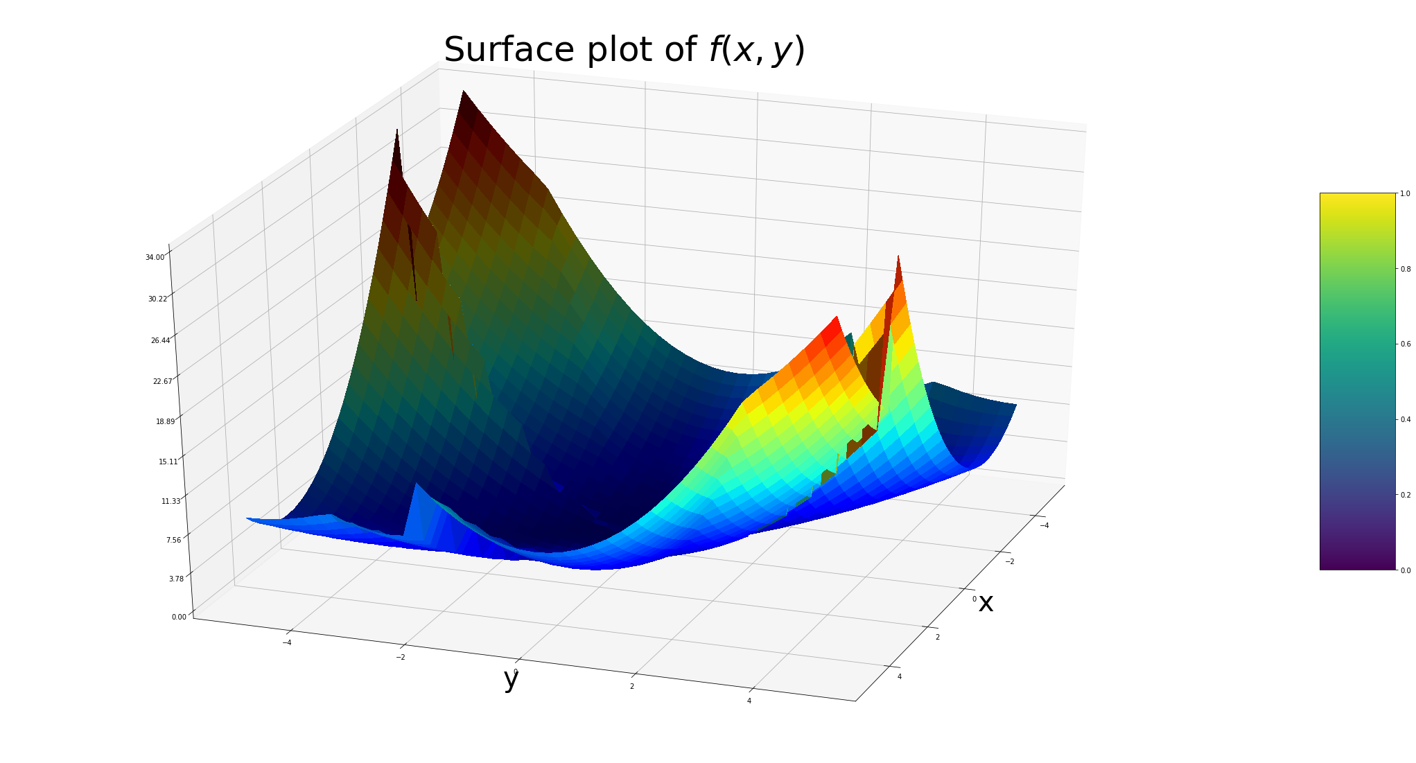
As a first step (and for the purposes of sanity check), we look at MKL-SGD in the simplest setting when there are no outliers and no noise. Recall from above that this means that 𝒘∗\boldsymbol{w^{*}} is in the optimal set of every single individual loss fi​(⋅)f_{i}(\cdot). However as mentioned above, even in this case the surrogate loss can be non-convex, as seen e.g. in Figure 1 for a simple example.
Refer to caption
Figure 1: Non-convexity of the surface plot with three samples in the two-dimensional noiseless linear regression setting

However, in the following lemma we show that even though the overall surrogate loss F~​(⋅)\tilde{F}(\cdot) is non-convex, in this no-noise no-outlier setting it has a special property with regards to the point 𝒘∗\boldsymbol{w^{*}}.

Lemma 1.

In the noiseless setting, for any 𝐰\boldsymbol{w} there exists a λ𝐰>0\lambda_{\boldsymbol{w}}>0 such that

∇F~(𝒘)⊤(𝒘−𝒘∗)≥λ𝒘‖𝒘−𝒘∗‖2.\nabla\widetilde{F}(\boldsymbol{w})^{\top}(\boldsymbol{w}-\boldsymbol{w^{*}})\geq\lambda_{\boldsymbol{w}}\norm{\w- \ws}^{2}.

In other words, what this lemma says is that on the line between any point 𝒘\boldsymbol{w} and the point 𝒘∗\boldsymbol{w^{*}}, the surrogate loss function F~\tilde{F} is convex from any point – even though it is not convex overall. This is akin to the restricted secant inequality condition described in [17, 37]. The following theorem uses this lemma to establish our first result: that in the noiseless setting with no outliers, 𝒘∗\boldsymbol{w^{*}} is the only fixed point (in expectation) of MKL-SGD.

Theorem 1 (Unique stationary point).

For the noiseless setting with no outliers, and under assumptions 1−31-3, the expected MKL-SGD update satisfies ∇F~​(𝐰)=0\nabla\widetilde{F}(\boldsymbol{w})=0 if and only if 𝐰=𝐰∗\boldsymbol{w}=\boldsymbol{w^{*}}.

4.2 Noiseless setting with Outliers

In presence of outliers, the surrogate loss can have multiple local minima that are far from 𝒘∗\boldsymbol{w^{*}} and indeed potentially even worse than what we could have obtained with vanilla SGD on the original loss function. We now analyze MKL-SGD in the simple setting of symmetric squared loss functions and try to gain useful insights into the landscape of loss function for the scalar setting. We would like to point out that the analysis in the next part serves as a clean template and can be extended for many other standard loss functions used in convex optimization.

Squared loss in the scalar setting

Figure 2 will be a handy tool for visualizing and understanding both the notation and results of this subsection. Consider the case where all losses are squared losses, with all the clean samples centered at w∗w^{*} and all the outliers at wBw_{B}, but all having different Lipschitz constants. Specifically, consider:

fi​(w)={li​(w−w∗)2∀i∉𝕆li​(w−wB)2∀i∈𝕆,\displaystyle f_{i}(w)=\begin{cases}&l_{i}(w-w^{*})^{2}\penalty\ \penalty\ \forall\penalty\ i\notin\mathbb{O}\\ &l_{i}(w-w_{B})^{2}\penalty\ \penalty\ \forall\penalty\ i\in\mathbb{O},\end{cases} (4)

Let lm:=mini∉𝕆⁡lil_{m}:=\min_{i\notin\mathbb{O}}l_{i} and Let lM:=maxi∈𝕆⁡lil_{M}:=\max_{i\in\mathbb{O}}l_{i} and lm​a​x=maxi∈[n]⁡lil_{max}=\max_{i\in[n]}l_{i}, lm​i​n=mini∈[n]⁡lil_{min}=\min_{i\in[n]}l_{i}. Let us define κ=lm​a​xlm​i​n≥lMlm\kappa=\dfrac{l_{max}}{l_{min}}\geq\dfrac{l_{M}}{l_{m}}. We initialize MKL-SGD at w0=wBw_{0}=w_{B}, a point where the losses of outlier samples are 0 and all the clean samples have non-zero losses. As a result at wBw_{B}, MKL-SGD has a tendency to pick all the outlier samples with a higher probability than any of the clean samples. This does not bode well for the algorithm since this implies that the final stationary point will be heavily influenced by outliers. Let w¯M​K​L\bar{w}_{MKL} be the stationary point of MKL-SGD for this scalar case when initialized at wBw_{B}.

Let us define w~\widetilde{w} as follows:

w~:={w∣w=minα⁡α​w∗+(1−α)​wB,α∈(0,1),flm​(w)=flM​(w)}\displaystyle\widetilde{w}:=\begin{cases}\begin{cases}w\mid&w=\min_{\alpha}\alpha w^{*}+(1-\alpha)w_{B},\alpha\in(0,1),\quad f_{l_{m}}(w)=f_{l_{M}}(w)\end{cases}\end{cases} (5)

Thus, w~\widetilde{w} is the closest point to wBw_{B} on the line joining wBw_{B} and w∗w^{*} where the loss function of one of the clean samples and one of the outliers intersect as illustrated in Figure 2.

By observation, we know for the above scalar case w~=lm​w∗+lM​wBlm+lM\widetilde{w}=\dfrac{\sqrt{l_{m}}w^{*}+\sqrt{l_{M}}w_{B}}{\sqrt{l_{m}}+\sqrt{l_{M}}}. Let p^​(𝒘0)=∑j∈𝕆pj​(𝒘0)\hat{p}(\boldsymbol{w}_{0})=\sum_{j\in\mathbb{O}}p_{j}(\boldsymbol{w}_{0}) represent the total probability of picking outliers at the starting point 𝒘0\boldsymbol{w}_{0}. The maximum possible value that can be attained p^\hat{p} over the entire landscape is given as:

p^m​a​x=maxw⁡p^​(𝒘)=∑i=1|𝕆|pmi​(𝒘)​(𝒘)\displaystyle\hat{p}_{max}=\max_{w}\hat{p}(\boldsymbol{w})=\sum_{i=1}^{\mathbb{|O|}}p_{m_{i}(\boldsymbol{w})}(\boldsymbol{w}) (6)

The next condition gives a sufficient condition to avoid all the bad local minima are avoided no matter where we initialize. For the simple scalar case, the condition is:

Condition 1.

p^m​a​x<11+κ​κ\hat{p}_{max}<\dfrac{1}{1+\kappa\sqrt{\kappa}}

Refer to caption
Figure 2: Illustration with conditions when bad local minima will or will not exist. Here, we demonstrate that even if we start at an initialization 𝒘𝓑\boldsymbol{w_{\mathcal{B}}} that assigns the highest probabilities to bad samples (red), it is possible to avoid the existence of a bad local minima if Condition 1 is satisfied. Recursively, we show in Lemma 2 that it is possible to avoid all bad local minima and reach a good local minima (where the good samples have the highest probabilities)

To further elaborate on this, for the loss functions and w~\widetilde{w} defined in equations (4) and (5) respectively, if condition 1 is not satisfied, then we cannot say anything about where MKL-SGD converges. However, if condition 1 holds true, then we are in Case 1 (Figure 2), i.e. the stationary point attained by MKL-SGD will be such that it is possible to avoid the existence of the first bad local minima. The first bad local minima occurs by solving the optimization problem where the top-|𝕆||\mathbb{O}| highest probabilities are assigned to the bad samples.

Following the above analysis recursively, we can show that all other subsequent bad local minimas are avoided as well, until we reach the local minima which assigns the largest (n−|𝕆|)(n-|\mathbb{O}|) probabilities to the clean samples22 2 Refer to Appendix section 8.2.3 for further details on this discussion. This indicates that irrespective of where we initialize in the 1​D1D landscape, we are bound to end up at a local minima with the highest probabilities assigned to the clean samples. In the latter part of this section, we will show that MKL-SGD solution attained when Case 1 holds is provably better than the SGD solution. However, if condition 1 is false (Case 2, Figure 2), then it is possible that MKL-SGD gets stuck at any one of the many local minimas that exist close to the outlier center wBw_{B} and we cannot say anything about the relative distance from 𝒘∗\boldsymbol{w^{*}}.

A key takeaway from the above condition is that for a fixed nn as κ\kappa increases, we can tolerate smaller p^\hat{p} and consequently smaller fraction of corruptions ϵ\epsilon. For a fixed ϵ\epsilon and nn, increasing the parameter kk (upto k<n2k<\frac{n}{2}) in MKL-SGD leads to an increase in p^\hat{p} and thus increasing kk can lead to the violation of the above condition. This happens because samples with lower loss will be picked with increasing probability as kk increases and as a result the propensity of MKL-SGD to converge towards the closest stationary point it encounters is higher.

Squared loss in the vector setting

The loss functions are redefined as follows:

fi​(𝒘)={li​‖𝒘−𝒘∗‖2∀i∉𝕆li​‖𝒘−𝒘bi‖2∀i∈𝕆,\displaystyle f_{i}(\boldsymbol{w})=\begin{cases}{}&l_{i}\norm{\w-\ws}^{2}\penalty\ \penalty\ \forall\penalty\ i\notin\mathbb{O}\\ &l_{i}\norm{\w-\w_{b_i}}^{2}\penalty\ \penalty\ \forall\penalty\ i\in\mathbb{O},\end{cases} (7)

Without loss of generality, assume that 2​δ<‖𝒘b1−𝒘∗‖≤‖𝒘b2−𝒘∗‖≤⋯≤‖𝒘b|𝕆|−𝒘∗‖2\delta<\norm{\w_{b_1}-\ws}\leq\norm{\w_{b_2}-\ws}\leq\dots\leq\norm{\w_{b_{|\mathbb{O}|}}-\ws} and γ=2​δ‖𝒘b|𝕆|−𝒘∗‖\gamma=\dfrac{2\delta}{\norm{\w_{b_{|\mathbb{O}|}}-\ws}}. Let 𝒘¯\bar{\boldsymbol{w}} be any stationary attained by MKL-SGD. Suppose θi,𝒘¯\theta_{i,\bar{\boldsymbol{w}}} be the angle between the line passing through 𝒘bi\boldsymbol{w}_{b_{i}} and 𝒘∗\boldsymbol{w^{*}} and the line connecting 𝒘¯\bar{\boldsymbol{w}} and 𝒘∗\boldsymbol{w^{*}}. Let us define θM,𝒘¯:=maxi⁡θi,𝒘¯\theta_{M,\bar{\boldsymbol{w}}}:=\max_{i}\theta_{i,\bar{\boldsymbol{w}}} Consider κ=maxi∈[n]⁡limini∈[n]⁡li\kappa=\dfrac{\max_{i\in[n]}l_{i}}{\min_{i\in[n]}l_{i}}. Let p^​(𝒘0)=∑j∈𝕆pj​(𝒘0)\hat{p}(\boldsymbol{w}_{0})=\sum_{j\in\mathbb{O}}p_{j}(\boldsymbol{w}_{0}) represent the total probability of picking outliers at the starting point 𝒘0\boldsymbol{w}_{0}. The maximum possible value that can be attained p^\hat{p} is given as:

p^m​a​x=maxw⁡p^​(𝒘)=∑i=1|𝕆|pmi​(𝒘)​(𝒘)\displaystyle\hat{p}_{max}=\max_{w}\hat{p}(\boldsymbol{w})=\sum_{i=1}^{\mathbb{|O|}}p_{m_{i}(\boldsymbol{w})}(\boldsymbol{w}) (8)

where for any 𝒘\boldsymbol{w}, pmi​(𝒘)​(𝒘)p_{m_{i}(\boldsymbol{w})}(\boldsymbol{w}) are ordered i.e. pm1​(𝒘)​(𝒘)>pm2​(𝒘)​(𝒘)>⋯>pmn​(𝒘)​(𝒘)p_{m_{1}(\boldsymbol{w})}(\boldsymbol{w})>p_{m_{2}(\boldsymbol{w})}(\boldsymbol{w})>\dots>p_{m_{n}(\boldsymbol{w})}(\boldsymbol{w}).

At 𝒘∗\boldsymbol{w^{*}}, by definition, we know that ∀i∉𝕆\forall\penalty\ i\notin\mathbb{O}, fi​(𝒘∗)=0f_{i}(\boldsymbol{w^{*}})=0 and ∀j∈𝕆\forall\penalty\ j\in\mathbb{O}, fj​(𝒘∗)>0f_{j}(\boldsymbol{w^{*}})>0. By continuity arguments, there exists a ball of radius r>0r>0 around 𝒘∗\boldsymbol{w^{*}}, ℬr​(𝒘∗)\mathcal{B}_{r}(\boldsymbol{w^{*}}), defined as follows:

ℬr​(𝒘∗)={𝒘∣fi(𝒘)<fj(𝒘)∀i∉𝕆,j∈𝕆,‖𝒘−𝒘∗‖≤r}\displaystyle\mathcal{B}_{r}(\boldsymbol{w^{*}})=\begin{cases}\begin{cases}{}\boldsymbol{w}\mid&f_{i}(\boldsymbol{w})<f_{j}(\boldsymbol{w})\penalty\ \forall\penalty\ i\notin\mathbb{O},\penalty\ j\in\mathbb{O},\\ &\norm{\w-\ws}\leq r\end{cases}\end{cases} (9)

In the subsequent lemma, we show that that it is possible to drift into the ball ℬr​(𝒘∗)\mathcal{B}_{r}(\boldsymbol{w^{*}}) where the clean samples have the highest probability or the lowest loss. 33 3 It is trivial to show the existence of a ball of radius r>0r>0 for any set of continuously differentiable fi(.)f_{i}(.).

Lemma 2.

Consider the loss function and ℬr​(𝐰∗)\mathcal{B}_{r}(\boldsymbol{w^{*}}) as defined in equations (7) and (9) respectively. Suppose q=cos⁡(θM,𝐰¯)γ−1+κ​cos⁡(θM,𝐰¯)γ>0q=\dfrac{\cos{\theta_{M,\bar{\w}}}}{\gamma}-1+\dfrac{\sqrt{\kappa}\cos{\theta_{M,\bar{\w}}}}{\gamma}>0 and p^m​a​x\hat{p}_{max} as defined in Equation (8) satisfies p^m​a​x≤11+κ​q\hat{p}_{max}\leq\dfrac{1}{1+\kappa q}. Starting from any initialization 𝐰0\boldsymbol{w}_{0}, for any stationary point 𝐰¯\bar{\boldsymbol{w}} attained by MKL-SGD, we have that 𝐰¯∈ℬr​(𝐰∗)\bar{\boldsymbol{w}}\in\mathcal{B}_{r}(\boldsymbol{w^{*}})

In other words, initializing at any point in the landscape, the final stationary point attained by MKL-SGD will inevitably assign the largest n−|𝕆|n-|\mathbb{O}| probabilities to the clean samples. The proof is availabe in Appendix Section 8.2.3. For the scalar case, d=1d=1, we have θj,𝒘¯=0​∀j\theta_{j,\bar{\boldsymbol{w}}}=0\penalty\ \forall\penalty\ j. If γ=1\gamma=1 and all the outliers are centered at the same point, then in the scalar setting the condition in Lemma 2 reduces to condition 1.

Note that, the above lemma leads to a very strong worst-case guarantee. It states that the farthest optimum will always be within a bowl of distance rr from 𝒘∗\boldsymbol{w^{*}} no matter where we initialize. Moreover, as long as the condition is satisfied no matter where the outliers lie (can be adversarially chosen), MKL-SGD always has the propensity to bring the iterates to a ball of radius rr around 𝒘∗\boldsymbol{w^{*}}. However, when the necessary conditions for its convergence are violated, the guarantees are initialization dependent. Thus, all the discussions in the rest of this section will be with respect to these worst case guarantees. However, as we see in the experimental section for both neural networks and linear regression, random initialization also seems to perform better than SGD.

Effect of κ\kappa

A direct result of Lemma 2 is that higher the condition number of the set of quadratic loss functions, lower is the fraction ϵ\epsilon of outliers the MKL-SGD can tolerate. This is because large κ\kappa results in a small value of 11+κ​q\dfrac{1}{1+\kappa q}. This implies that p^\hat{p} has to be small which in turn requires smaller fractions fo corruptions, ϵ\epsilon.

Effect of γ\gamma:

The relative distance of the outliers from 𝒘∗\boldsymbol{w^{*}} plays a critical role in the condition for Lemma 2. We know that γ∈(0,1]\gamma\in(0,1]. γ=1\gamma=1 implies the outliers are equidistant from the optimum 𝒘∗\boldsymbol{w^{*}}. Low values of γ\gamma lead to a large qq leading to the violation of the condition with p^\hat{p} (since RHS in the condition is very small), which implies that one bad outlier can guarantee that the condition in Lemma 2 are violated. The guarantees in the above lemma are only when the outliers are not adversarially chosen to lie at very high relative distances from 𝒘∗\boldsymbol{w^{*}}. One way to avoid the set of outliers far far away from the optimum is to have a filtering step at the start of the algorithm like the one in [9]. We will refer this in Experiments.

Effect of cos⁡(θj,𝒘¯)\cos{\theta_{j,\bar{\w}}}:

At first glance, it may seem that cos⁡(θj,𝒘¯)=0\cos{\theta_{j,\bar{\w}}}=0 may cause 1+κ​q<01+\kappa q<0 and since p^​(𝒘)>0\hat{p}(\boldsymbol{w})>0, the condition in Lemma 2 may never be satisfied. Since, the term cos⁡(θj,𝒘¯)\cos{\theta_{j,\bar{\w}}} shows up in the denominator of the loss associated with outlier centered at 𝒘bj\boldsymbol{w}_{b_{j}}. Thus, low values of cos⁡(θj,𝒘¯)\cos{\theta_{j,\bar{\w}}} implies high value of loss associated with the function centered at 𝒘bj\boldsymbol{w}_{b_{j}} which in turn implies the maximum probability attained by that sample can never be in the top-|𝕆||\mathbb{O}| probabilities for that 𝒘¯\bar{\boldsymbol{w}}.

Analysis for the general outlier setting:

In this part, we analyze the fixed point equations associated with MKL-SGD and SGD and try to understand the behavior in a ball ℬr​(𝐰∗)\mathcal{B}_{r}(\boldsymbol{w^{*}}) around the optimum? For the sake of simplicity, we will assume that ‖∇fi​(𝒘)‖≤G​∀i∈𝕆\norm{\nabla f_i(\bs{w})}\leq G\penalty\ \forall\penalty\ i\in\mathbb{O}. Next, we analyze the following two quantities: i) distance of 𝒘¯𝑺​𝑮​𝑫\boldsymbol{\bar{w}_{SGD}} from 𝒘∗\boldsymbol{w^{*}} and distance of the any of the solutions attained by 𝒘¯𝑴​𝑲​𝑳\boldsymbol{\bar{w}_{MKL}} from 𝒘∗\boldsymbol{w^{*}}.

Lemma 3.

Let 𝐰¯𝐒​𝐆​𝐃\boldsymbol{\bar{w}_{SGD}} indicate the solution attained SGD. Under assumptions 1-3, there exists an ϵ′\epsilon^{\prime} such that for all ϵ≤ϵ′\epsilon\leq\epsilon^{\prime},

ϵ​G≤(1−ϵ)​L​‖𝒘¯𝑺​𝑮​𝑫−𝒘∗‖\displaystyle\epsilon G\leq(1-\epsilon)L\norm{\wsgd- \ws}

Using Lemma 1, we will define λ\lambda as follows:

λ:=min𝒘⁡λ𝒘\displaystyle\lambda:=\min_{\boldsymbol{w}}\lambda_{\boldsymbol{w}} (10)

In Appendix Section 8.2.2, we show that λ>0\lambda>0, however the exact lower bounds for this λ\lambda are loss function dependent. Naively, λ𝒘=mini⁡pi​(𝒘)​λ\lambda_{\boldsymbol{w}}=\min_{i}p_{i}(\boldsymbol{w})\lambda

Lemma 4.

Let 𝐰¯𝐌​𝐊​𝐋\boldsymbol{\bar{w}_{MKL}} be any first order stationary point attained by MKL-SGD. Under assumptions 1-3, for a given ϵ<1\epsilon<1 and λ\lambda as defined in equation (10), there exists a k′k^{\prime} such that for all k≥k′k\geq k^{\prime},

‖𝒘¯𝑴​𝑲​𝑳−𝒘∗‖≤ϵk​Gλ\displaystyle\norm{\wsm-\ws}\leq\dfrac{\epsilon^{k}G}{\lambda}

Finally, we show that any solution attained by MKL-SGD is provably better than the solution attained by SGD. We would like to emphasize that this is a very strong result. The MKL-SGD has numerous local minima and here we show that even the worst44 4 farthest solution from 𝒘∗\boldsymbol{w^{*}} solution attained by MKL-SGD is closer to 𝒘∗\boldsymbol{w^{*}} than the solution attained by SGD. Let us define α⁡(ϵ,L,k,λ)=(1−ϵ)​L​ϵk−1λ\alpha(\epsilon,L,k,\lambda)=\dfrac{(1-\epsilon)L\epsilon^{k-1}}{\lambda}

Theorem 2.

Let 𝐰¯𝐒​𝐆​𝐃\boldsymbol{\bar{w}_{SGD}} and 𝐰¯𝐌​𝐊​𝐋\boldsymbol{\bar{w}_{MKL}} be the the stationary points attained by SGD and MKL-SGD algorithms respectively for the noiseless setting with outliers. Under assumptions 1-3, for any 𝐰¯𝐌​𝐊​𝐋∈ℬr​(𝐰∗)\boldsymbol{\bar{w}_{MKL}}\in\mathcal{B}_{r}(\boldsymbol{w^{*}}) and λ\lambda defined in equation (10), there exists an ϵ′\epsilon^{\prime} and k′k^{\prime} such that for all ϵ≤ϵ′\epsilon\leq\epsilon^{\prime} and k≥k′k\geq k^{\prime}, we have α⁡(ϵ,L,k,λ)<1\alpha(\epsilon,L,k,\lambda)<1 and,

‖𝒘¯𝑴​𝑲​𝑳−𝒘∗‖<α⁡(ϵ,L,k,λ)​‖𝒘¯𝑺​𝑮​𝑫−𝒘∗‖\displaystyle\norm{ \wsm- \ws}<\alpha(\epsilon,L,k,\lambda)\norm{ \wsgd- \ws} (11)

For squared loss in scalar setting, we claimed that for a fixed nn and ϵ\epsilon, using a large kk may not be a good idea. Here, however once we are in the ball, ℬr​(𝒘∗)\mathcal{B}_{r}(\boldsymbol{w^{*}}), using larger kk (any k<n2k<\dfrac{n}{2}), reduces α⁡(ϵ,L,k,λ)\alpha(\epsilon,L,k,\lambda) and allows MKL-SGD to get closer to 𝒘∗\boldsymbol{w^{*}}.

The conditions required in Lemma 2 and Theorem 2 enable us to provide guarantees for only a subset of relatively well-conditioned problems. We would like to emphasize that the bounds we obtain are worst case bounds and not in expectation. As we will note in the Section 6 and the Appendix, however these bounds may not be necessary, for standard convex optimization problems MKL-SGD easily outperforms SGD.

5 Convergence Rates

In this section, we go back to the in expectation convergence analysis which is standard for the stochastic settings. For smooth functions with strong convexity, [25, 26] provided guarantees for linear rate of convergence. We restate the theorem here and show that the theorem still holds for the non-convex landscape obtained by MKL-SGD in noiseless setting.

Lemma 5 (Linear Convergence [26]).

Let F⁡(𝐰)=𝔼⁡[fi​(𝐰)]F(\boldsymbol{w})=\mathbb{E}[f_{i}(\boldsymbol{\boldsymbol{w}})] be λ\lambda-strongly convex. Set σ2=𝔼⁡[‖∇fi​(𝐰∗)‖2]\sigma^{2}=\mathbb{E}[\|\nabla f_{i}(\boldsymbol{w^{*}})\|^{2}] with 𝐰∗:=a​r​g​m​i​n​F​(𝐰)\boldsymbol{w}^{*}:=argminF(\boldsymbol{w}). Suppose η≤1supiLi\eta\leq\dfrac{1}{\sup_{i}L_{i}}. Let 𝚫t=𝐰𝐭−𝐰∗\boldsymbol{\Delta}_{t}=\boldsymbol{w_{t}}-\boldsymbol{w^{*}}. After TT iterations, SGD satisfies:

𝔼⁡[‖𝚫T‖2]≤(1−2​η​C^)T​‖𝚫0‖2+η​Rσ\displaystyle\mathbb{E}\left[\|\boldsymbol{\Delta}_{T}\|^{2}\right]\leq(1-2\eta\hat{C})^{T}\|\boldsymbol{\Delta}_{0}\|^{2}+\eta R_{\sigma} (12)

where C^=λ⁡(1−η​supiLi)\hat{C}=\lambda(1-\eta\sup_{i}L_{i}) and Rσ=σ2C^R_{\sigma}=\dfrac{\sigma^{2}}{\hat{C}}.

In the noiseless setting, we have ‖∇fi​(𝒘∗)‖=0\|\nabla f_{i}(\boldsymbol{w^{*}})\|=0 and so σ:=0\sigma:=0. 𝒘∗\boldsymbol{w}^{*} in (12) is the same as 𝒘∗\boldsymbol{w}^{*} stated in Theorem 1. Even though above theorem is for SGD, it still can be applied to our algorithm 1. At each iteration there exists a parameter λ𝒘𝒕\lambda_{\boldsymbol{w_{t}}} that could be seen as the strong convexity parameter (c.f. Lemma 1). For MKL-SGD, the parameter λ\lambda in (12) should be λ=mint⁡λ𝒘t\lambda=\min_{t}\lambda_{\boldsymbol{w}_{t}}. Thus, MKL-SGD algorithm still guarantees linear convergence result but with an implication of slower speed of convergence than standard SGD.

However, Lemma 5 will not hold for MKL-SGD in noisy setting since there exists no strong convexity parameter. Even for noiseless setting, the rate of convergence for MKL-SGD given in Lemma 5 is not tight. The upper bound in (12) is loosely set to the constant λ:=mint⁡λ𝒘t\lambda:=\min_{t}\lambda_{\boldsymbol{w}_{t}} for all the iterations. We fix it by concretely looking at each iteration. We give a general bound for the any stochastic algorithm (c.f. Theorem 3) for both noiseless and noisy setting in absence and presence of outliers.

Theorem 3 (Distance to w∗\boldsymbol{w^{*}}).

Let 𝚫t=𝐰𝐭−𝐰∗\boldsymbol{\Delta}_{t}=\boldsymbol{w_{t}}-\boldsymbol{w^{*}}. Denote the strong convexity parameter λg​o​o​d\lambda_{good} for all the good samples. Let

ψ=2​ηt​λg​o​o​d​(1−ηt​supiLi)​mini∉𝕆​pi​(𝒘𝒕)\psi=2\eta_{t}\lambda_{good}(1-\eta_{t}\sup_{i}L_{i})\min_{i\notin\mathbb{O}}p_{i}(\boldsymbol{w_{t}})

Suppose at tt​ht^{th} iteration, the stepsize is set as ηt\eta_{t}, then conditioned on the current parameter 𝐰t\boldsymbol{w}_{t}, the expectation of the distance between the 𝐰t+1\boldsymbol{w}_{t+1} and 𝐰∗\boldsymbol{w^{*}} can be upper bounded as:

𝔼i​[‖𝚫t+1‖2|𝒘𝒕]≤\displaystyle\mathbb{E}_{i}\left[\norm{\bs{\Delta}_{t+1}}^{2}|\boldsymbol{w_{t}}\right]\leq (1−ψ)​‖𝚫t‖2+ηt​Rt\displaystyle\left(1-\psi\right)\|\boldsymbol{\Delta}_{t}\|^{2}+\eta_{t}R_{t} (13)

where

Rt=\displaystyle R_{t}= −2∑i∉𝕆pi(𝒘𝒕)⟨𝒘𝒕−𝒘∗,∇fi(𝒘∗)⟩+∑i∈𝕆pi(𝒘𝒕)(2ηt‖∇fi​(𝒘∗)‖2+ηt‖∇fi​(𝒘𝒕)‖2+2(fi(𝒘∗)−fi(𝒘𝒕)))\displaystyle-2\sum_{i\notin\mathbb{O}}p_{i}(\boldsymbol{w_{t}})\langle{\boldsymbol{w_{t}}-\boldsymbol{w^{*}},\nabla f_{i}(\boldsymbol{w^{*}})\rangle}+\sum_{i\in\mathbb{O}}p_{i}(\boldsymbol{w_{t}})\left(2\eta_{t}\norm{\nabla f_{i}( \wg)}^{2}+\eta_{t}\norm{\nabla f_{i}( \bs{w_{t}})}^{2}+2\left(f_{i}(\boldsymbol{w^{*}})-f_{i}(\boldsymbol{w_{t}})\right)\right)

Theorem 3 implies that for any stochastic algorithm in the both noisy and noiseless setting, outliers can make the upper bound (RtR_{t}) much worse as it produces an extra term (the third term in RtR_{t}). The third term in RtR_{t} has a lower bound that could be an increasing function of |𝕆||\mathbb{O}|. However, its impact can be reduced by appropriately setting pi​(𝒘𝒕)p_{i}(\boldsymbol{w_{t}}), for instance using a larger kk in MKL-SGD. In the appendix, we also provide a sufficient condition (Corollary 1 in the Appendix) when MKL-SGD is always better than standard SGD (in terms of its distance from 𝒘∗\boldsymbol{w^{*}} in expectation).

The convergence rate depends on the constant ψ∝mini∉𝕆⁡pi​(𝒘𝒕)\psi\propto\min_{i\notin\mathbb{O}}p_{i}(\boldsymbol{w_{t}}). Note that this term mini∉𝕆⁡pi​(𝒘𝒕)\min_{i\notin\mathbb{O}}p_{i}(\boldsymbol{w_{t}}) is not too small for our algorithm MKL-SGD since it is a minimum among all the good sample (not including the outliers). However, when compared with vanilla SGD where mini∉𝕆⁡pi​(𝒘𝒕)=1/N\min_{i\notin\mathbb{O}}p_{i}(\boldsymbol{w_{t}})=1/N, mini∉𝕆⁡pi​(𝒘𝒕)\min_{i\notin\mathbb{O}}p_{i}(\boldsymbol{w_{t}}) with pi​(𝒘𝒕)p_{i}(\boldsymbol{w_{t}}) defined in (3) for MKL-SGD, in some sense, could be smaller than 1/N1/N. For instance, in the experiments given in Figure 5 (a)-(c) (Appendix 8.4.1), the slope of SGD is steeper than MKL-SGD, which implies that ψ(M​K​L)<ψ(S​G​D)\psi^{(MKL)}<\psi^{(SGD)}.

To understand the residual term RtR_{t}. Let us take the noiseless setting with outliers for an example. We have ∇fi​(𝒘∗)=0\nabla f_{i}(\boldsymbol{w^{*}})=0 and fi​(𝒘∗)=0f_{i}(\boldsymbol{w^{*}})=0 for all i∉𝕆i\notin\mathbb{O}. But for i∈𝕆i\in\mathbb{O}, ∇fi​(𝒘∗)≠0\nabla f_{i}(\boldsymbol{w^{*}})\neq 0 and fi​(𝒘∗)≠0f_{i}(\boldsymbol{w^{*}})\neq 0. Then the term RtR_{t} can be reduced to

Rt=\displaystyle R_{t}= ∑i∈𝕆pi​(𝒘𝒕)​(2​ηt​‖∇fi​(𝒘∗)‖2+ηt​‖∇fi​(𝒘𝒕)‖2+2​(fi​(𝒘∗)−fi​(𝒘𝒕)))\displaystyle\sum_{i\in\mathbb{O}}p_{i}(\boldsymbol{w_{t}})\left(2\eta_{t}\norm{\nabla f_{i}( \wg)}^{2}+\eta_{t}\norm{\nabla f_{i}( \bs{w_{t}})}^{2}+2\left(f_{i}(\boldsymbol{w^{*}})-f_{i}(\boldsymbol{w_{t}})\right)\right) (14)

If we are at the same point 𝒘𝒕\boldsymbol{w_{t}} for both SGD and MKL-SGD and pi​(𝒘𝒕)<1Np_{i}(\boldsymbol{w_{t}})<\dfrac{1}{N} for i∈𝕆i\in\mathbb{O}, we have Rt(S​G​D)>Rt(M​K​L)R_{t}^{(SGD)}>R_{t}^{(MKL)}. It means that MKL-SGD could reach to a neighbor with a radius that is possibly smaller than vanilla SGD algorithm, with a rate proportional to mini∉𝕆⁡pi​(𝒘𝒕)\min_{i\notin\mathbb{O}}p_{i}(\boldsymbol{w_{t}}) but not necessarily faster than vanilla SGD.

Figure 3: Comparing the performance of MKL-SGD (k=2k=2) and SGD for different values of κ\kappa in noiseless and noisy linear regression against varying fraction of outliers.

6 Experiments

In this section, we compare the performance of MKL-SGD and SGD for synthetic datasets for linear regression and small-scale neural networks.

6.1 Linear Regression

For simple linear regression, we assume that XiX_{i} are sampled from normal distribution with different condition numbers. Xi∼𝒩⁡(0,𝑫)X_{i}\sim\mathcal{N}(0,\boldsymbol{D}) where 𝑫\boldsymbol{D} is a diagonal matrix such that D11=κD_{11}=\kappa and Di​i=1D_{ii}=1 for all ii). For the noisy case, we assume additive Gaussian noise with mean 00 and variance 11. We compare the performance of MKL-SGD and SGD for different values of κ\kappa (Fig. 3) under noiseless and noisy settings against varying levels of corruption ϵ\epsilon. It is important to note that different κ\kappa values correspond to different rates of convergence. To ensure fair comparison, we run the algorithms till the error values stop decaying and take the distance of 𝒘∗\boldsymbol{w^{*}} from the exponential moving average of the iterates.

Dataset MNIST CIFAR10
SGD MKL-SGD Oracle SGD MKL-SGD Oracle
0.10.1 96.76 96.49 98.52 79.1 81.94 84.56
0.20.2 92.54 95.76 98.33 72.29 77.77 84.40
0.30.3 85.77 95.96 98.16 63.96 66.49 84.66
0.40.4 71.95 94.20 97.98 52.4 53.57 84.42
Table 1: Comparing the test accuracy of SGD and MKL-SGD(k=5/3k=5/3) over MNIST and CIFAR-10 datasets in presence of corruptions via directed label noise.

6.2 Neural Networks

For deep learning experiments, our results are in presence of corruptions via the directed noise model. In this corruption model, all the samples of class aa that are in error are assigned the same wrong label bb. This is a stronger corruption model than corruption by random noise (results in Appendix). For the MKL-SGD algorithm, we run a more practical batched (size bb) variant such that if k=2k=2 the algorithm picks b/2b/2 samples out of bb sample loss evaluations. The oracle contains results obtained by running SGD over only non-corrupted samples. More experimental results on neural networks for MNIST and CIFAR10 datasets can be found in the Appendix.

MNIST:

We train standard 2 layer convolutional network on subsampled MNIST (50005000 samples with labels). We train over 80 epochs using an initial learning rate of 0.050.05 with the decaying schedule of factor 55 after every 3030 epochs. The results of the MNIST dataset are averaged over 5 runs.

CIFAR10:

We train Resnet-18 [13] on CIFAR-10 (5000050000 training samples with labels) for over 200200 epochs using an initial learning rate of 0.050.05 with the decaying schedule of factor 55 after every 9090 epochs. The reported accuracy is based on the true validation set. The results of the CIFAR-10 dataset are averaged over 33 runs.

Lastly, in Fig. 4, we show that for a neural network MKL-SGD typically has a higher training loss but smaller test loss which partially explains its superior generalization performance.

Figure 4: Comparing training loss, test loss and test accuracy of MKL-SGDand SGD. Parameters: ϵ=0.2\epsilon=0.2, k=2k=2, b=16b=16. The training loss is lower for SGD which means that SGD overfits to the noisy data. The lower test loss and higher accuracy demonstrates the robustness MKL-SGDprovides for corrupted data.

7 Conclusion and Future Work

In this paper, we propose MKL-SGD that is computationally inexpensive, has linear convergence (upto a certain neighborhood) and is robust against outliers. We analyze MKL-SGD algorithm under noiseless and noisy settings with and without outliers. MKL-SGD outperforms SGD in terms of generalization for both linear regression and neural network experiments. More importantly, MKL-SGD opens up a plethora of challenging questions with respect to understanding convex optimization in a non-convex landscape.

To ensure consistency, i.e. ‖𝒘¯𝑴​𝑲​𝑳−𝒘∗‖→0\norm{\wsm-\ws}\rightarrow 0, we require that k≥n​ϵ+1k\geq n\epsilon+1. In all other cases, there will be a non-zero contribution from the outliers which keeps the MKL-SGD solution from exactly converging to 𝒘∗\boldsymbol{w^{*}}. In this paper, we consider unknown ϵ\epsilon and thus kk should be treated as a hyperparameter. However, if we knew the fraction of corruption, then with the right kk and smart initialization, it is possible to guarantee consistency. For neural network experiments in the Appendix, we show that tuning kk as a hyperparameter can lead to significant improvements in performance in presence of outliers.

Preliminary experiments indicate that smarter initialization techniques can improve the performance of MKL-SGD. The obvious question then is to provide worst case guarantees for a larger subset of problems using smarter initialization techniques. It will be interesting to analyze the tradeoff between rates of convergence to MKL-SGD and its robustness to outliers. The worst case analysis in the noisy setting with and without outliers also remains an open problem.

References

  • Anaraki and Hughes [2014] Farhad Pourkamali Anaraki and Shannon Hughes. Memory and computation efficient pca via very sparse random projections. In International Conference on Machine Learning, pages 1341–1349, 2014.
  • Angluin and Laird [1988] Dana Angluin and Philip Laird. Learning from noisy examples. Machine Learning, 2(4):343–370, 1988.
  • Balakrishnan et al. [2017] Sivaraman Balakrishnan, Simon S Du, Jerry Li, and Aarti Singh. Computationally efficient robust sparse estimation in high dimensions. In Conference on Learning Theory, pages 169–212, 2017.
  • Bengio et al. [2009] Yoshua Bengio, Jérôme Louradour, Ronan Collobert, and Jason Weston. Curriculum learning. In Proceedings of the 26th annual international conference on machine learning, pages 41–48. ACM, 2009.
  • Bhatia et al. [2015] Kush Bhatia, Prateek Jain, and Purushottam Kar. Robust regression via hard thresholding. In Advances in Neural Information Processing Systems, pages 721–729, 2015.
  • Bhatia et al. [2017] Kush Bhatia, Prateek Jain, Parameswaran Kamalaruban, and Purushottam Kar. Consistent robust regression. In Advances in Neural Information Processing Systems, pages 2110–2119, 2017.
  • Charikar et al. [2017] Moses Charikar, Jacob Steinhardt, and Gregory Valiant. Learning from untrusted data. In Proceedings of the 49th Annual ACM SIGACT Symposium on Theory of Computing, pages 47–60. ACM, 2017.
  • Chen et al. [2013] Yudong Chen, Constantine Caramanis, and Shie Mannor. Robust sparse regression under adversarial corruption. In International Conference on Machine Learning, pages 774–782, 2013.
  • Diakonikolas et al. [2018] Ilias Diakonikolas, Gautam Kamath, Daniel M Kane, Jerry Li, Jacob Steinhardt, and Alistair Stewart. Sever: A robust meta-algorithm for stochastic optimization. arXiv preprint arXiv:1803.02815, 2018.
  • Diakonikolas et al. [2019] Ilias Diakonikolas, Gautam Kamath, Daniel Kane, Jerry Li, Ankur Moitra, and Alistair Stewart. Robust estimators in high-dimensions without the computational intractability. SIAM Journal on Computing, 48(2):742–864, 2019.
  • Freund et al. [1999] Yoav Freund, Robert Schapire, and Naoki Abe. A short introduction to boosting. Journal-Japanese Society For Artificial Intelligence, 14(771-780):1612, 1999.
  • Gunasekar et al. [2018] Suriya Gunasekar, Jason Lee, Daniel Soudry, and Nathan Srebro. Characterizing implicit bias in terms of optimization geometry. arXiv preprint arXiv:1802.08246, 2018.
  • He et al. [2016] Kaiming He, Xiangyu Zhang, Shaoqing Ren, and Jian Sun. Identity mappings in deep residual networks. In European conference on computer vision, pages 630–645. Springer, 2016.
  • Huber [2011] Peter J Huber. Robust statistics. Springer, 2011.
  • Jiang et al. [2017] Lu Jiang, Zhengyuan Zhou, Thomas Leung, Li-Jia Li, and Li Fei-Fei. Mentornet: Learning data-driven curriculum for very deep neural networks on corrupted labels. arXiv preprint arXiv:1712.05055, 2017.
  • Kahn and Marshall [1953] Herman Kahn and Andy W Marshall. Methods of reducing sample size in monte carlo computations. Journal of the Operations Research Society of America, 1(5):263–278, 1953.
  • Karimi et al. [2016] Hamed Karimi, Julie Nutini, and Mark Schmidt. Linear convergence of gradient and proximal-gradient methods under the polyak-łojasiewicz condition. In Joint European Conference on Machine Learning and Knowledge Discovery in Databases, pages 795–811. Springer, 2016.
  • Karmalkar et al. [2019] Sushrut Karmalkar, Adam Klivans, and Pravesh Kothari. List-decodable linear regression. In Advances in Neural Information Processing Systems, pages 7423–7432, 2019.
  • Katharopoulos and Fleuret [2018] Angelos Katharopoulos and François Fleuret. Not all samples are created equal: Deep learning with importance sampling. arXiv preprint arXiv:1803.00942, 2018.
  • Klivans et al. [2018] Adam Klivans, Pravesh K Kothari, and Raghu Meka. Efficient algorithms for outlier-robust regression. arXiv preprint arXiv:1803.03241, 2018.
  • Kumar et al. [2010] M Pawan Kumar, Benjamin Packer, and Daphne Koller. Self-paced learning for latent variable models. In Advances in Neural Information Processing Systems, pages 1189–1197, 2010.
  • Lai et al. [2016] Kevin A Lai, Anup B Rao, and Santosh Vempala. Agnostic estimation of mean and covariance. In 2016 IEEE 57th Annual Symposium on Foundations of Computer Science (FOCS), pages 665–674. IEEE, 2016.
  • Lee and Sidford [2013] Yin Tat Lee and Aaron Sidford. Efficient accelerated coordinate descent methods and faster algorithms for solving linear systems. In 2013 IEEE 54th Annual Symposium on Foundations of Computer Science, pages 147–156. IEEE, 2013.
  • Liu et al. [2018] Liu Liu, Yanyao Shen, Tianyang Li, and Constantine Caramanis. High dimensional robust sparse regression. arXiv preprint arXiv:1805.11643, 2018.
  • Moulines and Bach [2011] Eric Moulines and Francis R Bach. Non-asymptotic analysis of stochastic approximation algorithms for machine learning. In Advances in Neural Information Processing Systems, pages 451–459, 2011.
  • Needell et al. [2014] Deanna Needell, Rachel Ward, and Nati Srebro. Stochastic gradient descent, weighted sampling, and the randomized kaczmarz algorithm. In Advances in neural information processing systems, pages 1017–1025, 2014.
  • Owen [2007] Art B Owen. A robust hybrid of lasso and ridge regression. 2007.
  • Prasad et al. [2018] Adarsh Prasad, Arun Sai Suggala, Sivaraman Balakrishnan, and Pradeep Ravikumar. Robust estimation via robust gradient estimation. arXiv preprint arXiv:1802.06485, 2018.
  • Ren et al. [2018] Mengye Ren, Wenyuan Zeng, Bin Yang, and Raquel Urtasun. Learning to reweight examples for robust deep learning. arXiv preprint arXiv:1803.09050, 2018.
  • Rolnick et al. [2017] David Rolnick, Andreas Veit, Serge Belongie, and Nir Shavit. Deep learning is robust to massive label noise. arXiv preprint arXiv:1705.10694, 2017.
  • Rousseeuw [1984] Peter J Rousseeuw. Least median of squares regression. Journal of the American statistical association, 79(388):871–880, 1984.
  • Shen and Sanghavi [2019] Yanyao Shen and Sujay Sanghavi. Learning with bad training data via iterative trimmed loss minimization. In International Conference on Machine Learning, pages 5739–5748, 2019.
  • Strohmer and Vershynin [2009] Thomas Strohmer and Roman Vershynin. A randomized kaczmarz algorithm with exponential convergence. Journal of Fourier Analysis and Applications, 15(2):262, 2009.
  • Víšek et al. [2002] Jan Víšek et al. The least weighted squares ii. consistency and asymptotic normality. Bulletin of the Czech Econometric Society, 9, 2002.
  • Víšek [2006] Jan Ámos Víšek. The least trimmed squares. part i: Consistency. Kybernetika, 42(1):1–36, 2006.
  • Xu et al. [2009] Huan Xu, Constantine Caramanis, and Shie Mannor. Robust regression and lasso. In Advances in Neural Information Processing Systems, pages 1801–1808, 2009.
  • Zhang [2017] Hui Zhang. The restricted strong convexity revisited: analysis of equivalence to error bound and quadratic growth. Optimization Letters, 11(4):817–833, 2017.
  • Zhao and Zhang [2015] Peilin Zhao and Tong Zhang. Stochastic optimization with importance sampling for regularized loss minimization. In international conference on machine learning, pages 1–9, 2015.

8 Appendix

8.1 Additional Results for Section 3

The following lemma provides upper bounds on the expected gradient of the worst-possible MKL-SGD solution that lies in a ball around 𝒘∗\boldsymbol{w^{*}}. Simultaneously satisfying the following bound with the one in Lemma 3 may lead to an infeasible set of ϵ\epsilon and N′N^{\prime}. And thus we use Lemma 4 in conjunction with 3.

Lemma 6.

Let us assume that MKL-SGD converges to 𝐰¯𝐌​𝐊​𝐋\boldsymbol{\bar{w}_{MKL}}. For any 𝐰¯𝐌​𝐊​𝐋∈ℬr​(𝐰∗)\boldsymbol{\bar{w}_{MKL}}\in\mathcal{B}_{r}(\boldsymbol{w^{*}}) that satisfies assumptions N1, N2, A4 and A5, there exists N′≥NN^{\prime}\geq N and ϵ′≤ϵ\epsilon^{\prime}\leq\epsilon such that,

‖∑i∉𝕆pi(𝒘¯𝑴​𝑲​𝑳)∇fi(𝒘¯𝑴​𝑲​𝑳)‖≤min⁡{(1−ϵk)​L​‖𝒘¯𝑴​𝑲​𝑳−𝒘∗‖,ϵk​G​(𝒘)}\displaystyle\norm{\sum_{i\notin\mathbb{O}} p_i(\wsm) \nabla f_i(\wsm)}\leq\min\left\{(1-\epsilon^{k})L\norm{\wsm- \ws},\epsilon^{k}G(\boldsymbol{w})\right\}

The proof for lemma 2 can be found in the Appendix Section 8.2.7

8.2 Proofs and supporting lemmas

8.2.1 Proof of Lemma 1

Proof.

F~​(𝒘)=∑ipmi​(𝒘)​(𝒘)\widetilde{F}(\boldsymbol{w})=\sum_{i}p_{m_{i}(\boldsymbol{w})}(\boldsymbol{w}). Let us fix a 𝒘\boldsymbol{w} such that pi=pi​(𝒘)p_{i}=p_{i}(\boldsymbol{w}). We know that for any pip_{i}, ∑ipi​fi​(𝒘)\sum_{i}p_{i}f_{i}(\boldsymbol{w}) is strongly convex in 𝒘\boldsymbol{w} with parameter λ𝒘\lambda_{\boldsymbol{w}}. This implies

∇F~(𝒘)⊤(𝒘−𝒘∗)≥λ𝒘‖𝒘−𝒘∗‖2\nabla\widetilde{F}(\boldsymbol{w})^{\top}(\boldsymbol{w}-\boldsymbol{w^{*}})\geq\lambda_{\boldsymbol{w}}\norm{\bs{w} - \ws}^{2}

∎

A naive bound for the above Lemma can be:

∇F~(𝒘)⊤(𝒘−𝒘∗)≥minipi∑ifi(𝒘)≥λ​mini​pi⏟λ𝒘‖𝒘−𝒘∗‖2\nabla\widetilde{F}(\boldsymbol{w})^{\top}(\boldsymbol{w}-\boldsymbol{w^{*}})\geq\min_{i}p_{i}\sum_{i}f_{i}(\boldsymbol{w})\geq\underbrace{\lambda\min_{i}p_{i}}_{\lambda_{\boldsymbol{w}}}\norm{\bs{w} - \ws}^{2}

8.2.2 Proof of Theorem 1

Proof.

By the definition of the noiseless framework, 𝒘∗\boldsymbol{w^{*}} is the unique optimum of F⁡(𝒘)F(\boldsymbol{w}) and lies in the optimal set of each fi(.)f_{i}(.). We will prove this theorem by contradiction. Assume there exists some 𝒘^≠𝒘∗\hat{\boldsymbol{w}}\neq\boldsymbol{w^{*}} that also satisfies optimum of ∇F~​(𝒘^)=𝟎\nabla\widetilde{F}(\hat{\boldsymbol{w}})=\boldsymbol{0}. At 𝒘^\hat{\boldsymbol{w}}, we have 0=<∇F~​(𝒘^),𝒘^−𝒘∗>=λ​‖𝒘^−𝒘∗‖20=<\nabla\widetilde{F}(\hat{\boldsymbol{w}}),\hat{\boldsymbol{w}}-\boldsymbol{w^{*}}>=\lambda\norm{\hat{\w} - \ws}^{2}. This implies 𝒘^=𝒘∗\hat{\boldsymbol{w}}=\boldsymbol{w^{*}}. ∎

Theorem 1 and Assumption 2 guarantee that λ𝒘>0\lambda_{\boldsymbol{w}}>0. If f⁡(𝒘)f(\boldsymbol{w}) is strongly convex and g⁡(𝒘)g(\boldsymbol{w}) is convex, then we know that f⁡(𝒘)+g⁡(𝒘)f(\boldsymbol{w})+g(\boldsymbol{w}) is strongly convex. On similar lines we can show that λ>0\lambda>0 by splitting the terms in F⁡(𝒘)~\tilde{F(\boldsymbol{w})} as pm​i​n​F​(𝒘)p_{min}F(\boldsymbol{w}) and (F~​(𝒘)−pm​i​n​F​(𝒘))(\tilde{F}(\boldsymbol{w})-p_{min}F(\boldsymbol{w})). The first term has λ>0\lambda>0 (Assumption 2) and the second term has λ=0\lambda=0 (since it is convex). Note, pm​i​np_{min} is a positive constant independent of 𝒘\boldsymbol{w} and so the above lemma is for all 𝒘\boldsymbol{w}.

8.2.3 Proof of Lemma 2

Let 𝒘¯\bar{\boldsymbol{w}} be a stationary point of MKL-SGD. Now, we analyze the loss landscape on the line joining 𝒘∗\boldsymbol{w^{*}} and 𝒘C\boldsymbol{w}_{C} where 𝒘C=C​𝒘¯\boldsymbol{w}_{C}=C\bar{\boldsymbol{w}} is any arbitrary point 55 5 Note that we just need 𝒘C\boldsymbol{w}_{C} for the purpose of landscape analysis and it is not a parameter of the algorithm in the landscape at a distance as far as the farthest outlier from 𝒘∗\boldsymbol{w^{*}}. Let CC be a very large number.

The loss functions and 𝒘~\widetilde{\boldsymbol{w}} are redefined as follows:

fi​(𝒘)={li​‖𝒘−𝒘∗‖2∀i∈𝕆li​‖𝒘−𝒘bi‖2∀i∉𝕆,\displaystyle f_{i}(\boldsymbol{w})=\begin{cases}{}&l_{i}\norm{\w-\ws}^{2}\penalty\ \penalty\ \forall\penalty\ i\in\mathbb{O}\\ &l_{i}\norm{\w-\w_{b_i}}^{2}\penalty\ \penalty\ \forall\penalty\ i\notin\mathbb{O},\end{cases}
𝒘~:={𝒘|𝒘=minα∈(0,1)⁡α​𝒘∗+(1−α)​𝒘C,flm​(𝒘)=flM​(𝒘)}\displaystyle\widetilde{\boldsymbol{w}}:=\begin{cases}\begin{cases}\boldsymbol{w}\bigg|&\boldsymbol{w}=\min_{\alpha\in(0,1)}\alpha\boldsymbol{w^{*}}+(1-\alpha)\boldsymbol{w}_{C},\\ &f_{l_{m}}(\boldsymbol{w})=f_{l_{M}}(\boldsymbol{w})\end{cases}\end{cases}

where |𝕆|=b\absolutevalue{\mathbb{O}}=b such that n=g+bn=g+b. Let lm=mini∉𝕆⁡lil_{m}=\min_{i\notin\mathbb{O}}l_{i} and Let lM=maxi∈𝕆⁡lil_{M}=\max_{i\in\mathbb{O}}l_{i} and lm​a​x=mini∈[n]⁡lil_{max}=\min_{i\in[n]}l_{i}, lm​i​n=mini∈[n]⁡lil_{min}=\min_{i\in[n]}l_{i}. Let us define κ=lm​a​xlm​i​n≥lMlm\kappa=\dfrac{l_{max}}{l_{min}}\geq\dfrac{l_{M}}{l_{m}}.

Now at w¯\bar{w}, we have ∇F~​(𝒘¯)=0\nabla\widetilde{F}(\bar{\boldsymbol{w}})=0. Let us assume that the outliers are chosen in such a way that at 𝒘C\boldsymbol{w}_{C}, all the outliers have the lowest loss. As stated in the previous lemma, the results hold irrespective of that. This implies:

∑i∉𝕆pi(𝒘C)∇fi(𝒘¯)\displaystyle\sum_{i\notin\mathbb{O}}p_{i}(\boldsymbol{w}_{C})\nabla f_{i}(\bar{\boldsymbol{w}}) =−∑j∈𝕆pj(𝒘C)∇fj(𝒘¯)\displaystyle=-\sum_{j\in\mathbb{O}}p_{j}(\boldsymbol{w}_{C})\nabla f_{j}(\bar{\boldsymbol{w}})
∑i∉𝕆pi​(𝒘C)​li​(𝒘¯−𝒘∗)\displaystyle\sum_{i\notin\mathbb{O}}p_{i}(\boldsymbol{w}_{C})l_{i}(\bar{\boldsymbol{w}}-\boldsymbol{w^{*}}) =−∑j∈𝕆pj(𝒘C)lj(𝒘¯−𝒘bj)\displaystyle=-\sum_{j\in\mathbb{O}}p_{j}(\boldsymbol{w}_{C})l_{j}(\bar{\boldsymbol{w}}-\boldsymbol{w}_{b_{j}})
𝒘¯\displaystyle\bar{\boldsymbol{w}} =∑i∉𝕆pi​(𝒘C)​li​𝒘∗+∑j∈𝕆pj​(𝒘C)​lj​𝒘bj∑i∉𝕆pi​(𝒘C)​li+∑j∈𝕆pj​(𝒘C)​lj\displaystyle=\dfrac{\sum_{i\notin\mathbb{O}}p_{i}(\boldsymbol{w}_{C})l_{i}\boldsymbol{w^{*}}+\sum_{j\in\mathbb{O}}p_{j}(\boldsymbol{w}_{C})l_{j}\boldsymbol{w}_{b_{j}}}{\sum_{i\notin\mathbb{O}}p_{i}(\boldsymbol{w}_{C})l_{i}+\sum_{j\in\mathbb{O}}p_{j}(\boldsymbol{w}_{C})l_{j}}
By triangle inequality, ​‖𝒘¯−𝒘∗‖\displaystyle\text{By triangle inequality, }\norm{\bar{\w} - \ws} ≤∑j∈𝕆pj​(𝒘C)​lj​‖𝒘bj−𝒘∗‖∑i∉𝕆pi​(𝒘C)​li+∑j∈𝕆pj​(𝒘C)​lj\displaystyle\leq\dfrac{\sum_{j\in\mathbb{O}}p_{j}(\boldsymbol{w}_{C})l_{j}\norm{\w_{b_j}-\ws}}{\sum_{i\notin\mathbb{O}}p_{i}(\boldsymbol{w}_{C})l_{i}+\sum_{j\in\mathbb{O}}p_{j}(\boldsymbol{w}_{C})l_{j}}

Without loss of generality assume that the outliers are ordered as follows: ‖𝒘b1−𝒘∗‖≤‖𝒘b2−𝒘∗‖≤⋯≤‖𝒘b|𝕆|−𝒘∗‖\norm{\w_{b_1}-\ws}\leq\norm{\w_{b_2}-\ws}\leq\dots\leq\norm{\w_{b_{|\mathbb{O}|}}-\ws}.

Now 𝒘~\widetilde{\boldsymbol{w}} be some point of intersection of function in the set of clean samples and a function in the set of outliers to 𝒘∗\boldsymbol{w^{*}}. Let θj\theta_{j} be the angle between the line connecting 𝒘bj\boldsymbol{w}_{b_{j}} and 𝒘∗\boldsymbol{w^{*}} to the line connecting 𝒘C\boldsymbol{w}_{C} to 𝒘∗\boldsymbol{w^{*}}. For any two curves with Lipschitz constants lil_{i} and ljl_{j}, the halfspaces passing through the weighted mean are also the region where both functions have equal values.

Thus,

𝒘~=li​𝒘∗+lj​𝒘bjli+lj\widetilde{\boldsymbol{w}}=\dfrac{\sqrt{l_{i}}\boldsymbol{w^{*}}+\sqrt{l_{j}}\boldsymbol{w}_{b_{j}}}{\sqrt{l_{i}}+\sqrt{l_{j}}}

.

‖𝒘~−𝒘∗‖\displaystyle\norm{\widetilde{\w} -\ws} =lj​‖𝒘bj−𝒘∗‖lj+li\displaystyle=\dfrac{\sqrt{l_{j}}\norm{\w_{b_j}-\ws}}{\sqrt{l_{j}}+\sqrt{l_{i}}}

Let γ\gamma denote the following ratio:

γ=minj∈𝕆⁡‖𝒘bj−𝒘∗‖maxj∈𝕆⁡‖𝒘bj−𝒘∗‖=2​δδm​a​x\gamma=\dfrac{\min_{j\in\mathbb{O}}\norm{\w_{b_j}-\ws}}{\max_{j\in\mathbb{O}}\norm{\w_{b_j}-\ws}}=\dfrac{2\delta}{\delta_{max}}

Now, we want:

∑j∈𝕆pj​(𝒘C)​lj​‖𝒘bj−𝒘∗‖∑i∉𝕆pi​(𝒘C)​li+∑j∈𝕆pj​(𝒘C)​lj\displaystyle{}\dfrac{\sum_{j\in\mathbb{O}}p_{j}(\boldsymbol{w}_{C})l_{j}\norm{\w_{b_j}-\ws}}{\sum_{i\notin\mathbb{O}}p_{i}(\boldsymbol{w}_{C})l_{i}+\sum_{j\in\mathbb{O}}p_{j}(\boldsymbol{w}_{C})l_{j}} ≤ltjltj+lg​‖𝒘bj−𝒘∗‖cos⁡(θj)=‖𝒘~−𝒘∗‖cos⁡(θj)\displaystyle\leq\dfrac{\sqrt{l_{t_{j}}}}{\sqrt{l_{t_{j}}}+\sqrt{l_{g}}}\dfrac{\norm{\w_{b_j}-\ws}}{\cos{\theta_j}}=\dfrac{\norm{\widetilde{\w} -\ws}}{\cos{\theta_j}}
∑j∈𝕆pj​(𝒘C)​lj​‖𝒘bj−𝒘∗‖∑i∉𝕆pi​(𝒘C)​li+∑j∈𝕆pj​(𝒘C)​lj≤∑j∈𝕆pj​(𝒘C)​lj​‖𝒘b|𝕆|−𝒘∗‖∑i∉𝕆pi​(𝒘C)​li+∑j∈𝕆pj​(𝒘C)​lj\displaystyle\dfrac{\sum_{j\in\mathbb{O}}p_{j}(\boldsymbol{w}_{C})l_{j}\norm{\w_{b_j}-\ws}}{\sum_{i\notin\mathbb{O}}p_{i}(\boldsymbol{w}_{C})l_{i}+\sum_{j\in\mathbb{O}}p_{j}(\boldsymbol{w}_{C})l_{j}}\leq\dfrac{\sum_{j\in\mathbb{O}}p_{j}(\boldsymbol{w}_{C})l_{j}\norm{\w_{b_{|\mathbb{O}|}}-\ws}}{\sum_{i\notin\mathbb{O}}p_{i}(\boldsymbol{w}_{C})l_{i}+\sum_{j\in\mathbb{O}}p_{j}(\boldsymbol{w}_{C})l_{j}} ≤ltjltj+lg​‖𝒘bj−𝒘∗‖cos⁡(θj)\displaystyle\leq\dfrac{\sqrt{l_{t_{j}}}}{\sqrt{l_{t_{j}}}+\sqrt{l_{g}}}\dfrac{\norm{\w_{b_j}-\ws}}{\cos{\theta_j}}
∑j∈𝕆pj​(𝒘C)​lj∑i∉𝕆pi​(𝒘C)​li+∑j∈𝕆pj​(𝒘C)​lj\displaystyle\dfrac{\sum_{j\in\mathbb{O}}p_{j}(\boldsymbol{w}_{C})l_{j}}{\sum_{i\notin\mathbb{O}}p_{i}(\boldsymbol{w}_{C})l_{i}+\sum_{j\in\mathbb{O}}p_{j}(\boldsymbol{w}_{C})l_{j}} ≤ltjltj+lg​‖𝒘bj−𝒘∗‖cos⁡(θj)​‖𝒘b|𝕆|−𝒘∗‖\displaystyle\leq\dfrac{\sqrt{l_{t_{j}}}}{\sqrt{l_{t_{j}}}+\sqrt{l_{g}}}\dfrac{\norm{\w_{b_j}-\ws}}{\cos{\theta_j}\norm{\w_{b_{|\mathbb{O}|}}-\ws}}
∑j∈𝕆pj​(𝒘C)​lj∑i∉𝕆pi​(𝒘C)​li+∑j∈𝕆pj​(𝒘C)​lj\displaystyle\dfrac{\sum_{j\in\mathbb{O}}p_{j}(\boldsymbol{w}_{C})l_{j}}{\sum_{i\notin\mathbb{O}}p_{i}(\boldsymbol{w}_{C})l_{i}+\sum_{j\in\mathbb{O}}p_{j}(\boldsymbol{w}_{C})l_{j}} ≤ltjltj+lg​γcos⁡(θj)\displaystyle\leq\dfrac{\sqrt{l_{t_{j}}}}{\sqrt{l_{t_{j}}}+\sqrt{l_{g}}}\dfrac{\gamma}{\cos{\theta_j}}

For simplicity, Γ=γcos⁡(θj)\Gamma=\dfrac{\gamma}{\cos{\theta_j}}, then we have:

∑j∈𝕆pj​(𝒘C)​lj∑i∉𝕆pi​(𝒘C)​li+∑j∈𝕆pj​(𝒘C)​lj\displaystyle{}\dfrac{\sum_{j\in\mathbb{O}}p_{j}(\boldsymbol{w}_{C})l_{j}}{\sum_{i\notin\mathbb{O}}p_{i}(\boldsymbol{w}_{C})l_{i}+\sum_{j\in\mathbb{O}}p_{j}(\boldsymbol{w}_{C})l_{j}} ≤ltjltj+lg​Γ\displaystyle\leq\dfrac{\sqrt{l_{t_{j}}}}{\sqrt{l_{t_{j}}}+\sqrt{l_{g}}}\Gamma
1Γ​(lgltj+1)−1\displaystyle\dfrac{1}{\Gamma}\left(\dfrac{\sqrt{l_{g}}}{\sqrt{l_{t_{j}}}}+1\right)-1 ≤(1−p^)​lmp^​lM≤∑i∉𝕆pi​(𝒘C)​li∑j∈𝕆pj​(𝒘C)​lj\displaystyle\leq\dfrac{(1-\hat{p})l_{m}}{\hat{p}l_{M}}\leq\dfrac{\sum_{i\notin\mathbb{O}}p_{i}(\boldsymbol{w}_{C})l_{i}}{\sum_{j\in\mathbb{O}}p_{j}(\boldsymbol{w}_{C})l_{j}}
p^1−p^\displaystyle\dfrac{\hat{p}}{1-\hat{p}} ≤lmlM1Γ−1+1Γ​lgltj\displaystyle\leq\dfrac{\frac{l_{m}}{l_{M}}}{\frac{1}{\Gamma}-1+\frac{1}{\Gamma}\frac{\sqrt{l_{g}}}{\sqrt{l_{t_{j}}}}}
p^\displaystyle\hat{p} ≤11+κ⁡(1Γ−1+κΓ)≤11+lMlm​(1Γ−1+1Γ​lgltj)\displaystyle\leq\dfrac{1}{1+\kappa\left(\frac{1}{\Gamma}-1+\frac{\sqrt{\kappa}}{\Gamma}\right)}\leq\dfrac{1}{1+\frac{l_{M}}{l_{m}}\left(\frac{1}{\Gamma}-1+\frac{1}{\Gamma}\frac{\sqrt{l_{g}}}{\sqrt{l_{t_{j}}}}\right)}

Replacing Γ=γminj⁡cos⁡(θj)\Gamma=\dfrac{\gamma}{\min_{j}\cos{\theta_j}}, and let q=cos⁡(θj)γ−1+cos⁡(θj)​κγq=\frac{\cos{\theta_j}}{\gamma}-1+\frac{\cos{\theta_j}\sqrt{\kappa}}{\gamma} the condition to guarantee that bad local minima do no exist is p^≤11+κ​q\hat{p}\leq\dfrac{1}{1+\kappa q} and q>0q>0. Now, we can repeat the above analysis recursively for every corresponding 𝒘C\boldsymbol{w}_{C} and 𝒘~\tilde{\boldsymbol{w}} in the landscape and so now θj\theta_{j} is a function of 𝒘~\tilde{\boldsymbol{w}} as well as is represented in the theorem statement.

Note: In the vector case, for example there exists a fine tradeoff between how large θj\theta_{j} can be and if for large θj\theta_{j}, the loss corresponding to the outlier will be one of the lowest. Understanding that tradeoff is beyond the scope of this paper.

8.2.4 Proof of Lemma 3

Proof.

At 𝒘¯𝑺​𝑮​𝑫\boldsymbol{\bar{w}_{SGD}}, ∇F~​(𝒘¯𝑺​𝑮​𝑫)=0\nabla\widetilde{F}(\boldsymbol{\bar{w}_{SGD}})=0. Then,

∑i∉𝕆∇fi​(𝒘¯𝑺​𝑮​𝑫)\displaystyle\sum_{i\notin\mathbb{O}}\nabla f_{i}(\boldsymbol{\bar{w}_{SGD}}) =−∑i∈𝒪∇fi(𝒘¯𝑺​𝑮​𝑫)\displaystyle=-\sum_{i\in\mathcal{O}}\nabla f_{i}(\boldsymbol{\bar{w}_{SGD}})
‖∑i∉𝕆∇fi​(𝒘¯𝑺​𝑮​𝑫)‖\displaystyle\norm{\sum_{i\notin\mathbb{O}} \nabla f_i(\wsgd) } =‖∑i∈𝒪∇fi​(𝒘¯𝑺​𝑮​𝑫)‖\displaystyle=\norm{ \sum_{i\in\mathcal{O}} \nabla f_i(\wsgd)}
‖∑i∉𝕆∇fi​(𝒘¯𝑺​𝑮​𝑫)‖\displaystyle\norm{\sum_{i\notin\mathbb{O}} \nabla f_i(\wsgd)} ≤∑i‖∇fi​(𝒘¯𝑺​𝑮​𝑫)‖\displaystyle\leq\sum_{i}\norm{\nabla f_i(\wsgd)}
≤∑iL​‖𝒘¯𝑺​𝑮​𝑫−𝒘∗‖\displaystyle\leq\sum_{i}L\norm{\wsgd- \ws}
=(1−ϵ)​n​L​‖𝒘¯𝑺​𝑮​𝑫−𝒘∗‖\displaystyle=(1-\epsilon)nL\norm{\wsgd- \ws} (15)
‖∑i∈𝒪∇fi​(𝒘¯𝑺​𝑮​𝑫)‖\displaystyle\norm{ \sum_{i\in\mathcal{O}} \nabla f_i(\wsgd)} ≤∑i∈𝒪‖∇fi​(𝒘¯𝑺​𝑮​𝑫)‖\displaystyle\leq\sum_{i\in\mathcal{O}}\norm{ \nabla f_i(\wsgd)}
≤∑i∈𝒪G⁡(𝒘¯𝑺​𝑮​𝑫)\displaystyle\leq\sum_{i\in\mathcal{O}}G(\boldsymbol{\bar{w}_{SGD}})
≤ϵ​G​(𝒘¯𝑺​𝑮​𝑫)\displaystyle\leq\epsilon G(\boldsymbol{\bar{w}_{SGD}}) (16)
‖∑i∈𝒪∇fi​(𝒘¯𝑺​𝑮​𝑫)‖=min⁡(ϵ​n​G​(𝒘¯𝑺​𝑮​𝑫),(1−ϵ)​n​L​‖𝒘¯𝑺​𝑮​𝑫−𝒘∗‖)\norm{ \sum_{i\in\mathcal{O}} \nabla f_i(\wsgd)}=\min\left(\epsilon nG(\boldsymbol{\bar{w}_{SGD}}),(1-\epsilon)nL\norm{\wsgd- \ws}\right)

∎

8.2.5 Proof of Lemma 4

Proof.

At 𝒘¯𝑴​𝑲​𝑳\boldsymbol{\bar{w}_{MKL}}, ∇F~​(𝒘¯𝑴​𝑲​𝑳)=0\nabla\widetilde{F}(\boldsymbol{\bar{w}_{MKL}})=0. This implies

∑i∉𝕆pi(𝒘¯𝑴​𝑲​𝑳)∇fi(𝒘¯𝑴​𝑲​𝑳)\displaystyle\sum_{i\notin\mathbb{O}}p_{i}(\boldsymbol{\bar{w}_{MKL}})\nabla f_{i}(\boldsymbol{\bar{w}_{MKL}}) =−∑i∈𝒪pi(𝒘¯𝑴​𝑲​𝑳)∇fi(𝒘¯𝑴​𝑲​𝑳)\displaystyle=-\sum_{i\in\mathcal{O}}p_{i}(\boldsymbol{\bar{w}_{MKL}})\nabla f_{i}(\boldsymbol{\bar{w}_{MKL}})
Multiplying both sides by ​(𝒘¯𝑴​𝑲​𝑳−𝒘∗)\displaystyle\text{Multiplying both sides by }(\boldsymbol{\bar{w}_{MKL}}-\boldsymbol{w^{*}})\qquad
∑i∉𝕆pi​(𝒘¯𝑴​𝑲​𝑳)<∇fi​(𝒘¯𝑴​𝑲​𝑳),𝒘¯𝑴​𝑲​𝑳−𝒘∗>\displaystyle\sum_{i\notin\mathbb{O}}p_{i}(\boldsymbol{\bar{w}_{MKL}})<\nabla f_{i}(\boldsymbol{\bar{w}_{MKL}}),\boldsymbol{\bar{w}_{MKL}}-\boldsymbol{w^{*}}> =−∑i∈𝒪pi(𝒘¯𝑴​𝑲​𝑳)<∇fi(𝒘¯𝑴​𝑲​𝑳),𝒘¯𝑴​𝑲​𝑳−𝒘∗>\displaystyle=-\sum_{i\in\mathcal{O}}p_{i}(\boldsymbol{\bar{w}_{MKL}})<\nabla f_{i}(\boldsymbol{\bar{w}_{MKL}}),\boldsymbol{\bar{w}_{MKL}}-\boldsymbol{w^{*}}> (17)
<∇F~𝒢(𝒘¯𝑴​𝑲​𝑳),𝒘¯𝑴​𝑲​𝑳−𝒘∗>\displaystyle<\nabla\widetilde{F}_{\mathcal{G}}(\boldsymbol{\bar{w}_{MKL}}),\boldsymbol{\bar{w}_{MKL}}-\boldsymbol{w^{*}}> =−∑i∈𝒪pi(𝒘¯𝑴​𝑲​𝑳)<∇fi(𝒘¯𝑴​𝑲​𝑳),𝒘¯𝑴​𝑲​𝑳−𝒘∗>\displaystyle=-\sum_{i\in\mathcal{O}}p_{i}(\boldsymbol{\bar{w}_{MKL}})<\nabla f_{i}(\boldsymbol{\bar{w}_{MKL}}),\boldsymbol{\bar{w}_{MKL}}-\boldsymbol{w^{*}}>
Lower bounding the LHS using Lemma 1 and m=m⁡(𝒘¯𝑴​𝑲​𝑳)\displaystyle m=m(\boldsymbol{\bar{w}_{MKL}}) , (18)
m​‖𝒘¯𝑴​𝑲​𝑳−𝒘∗‖2\displaystyle m\norm{ \wsm- \ws}^{2} ≤‖<∇F~𝒢(𝒘¯𝑴​𝑲​𝑳),𝒘¯𝑴​𝑲​𝑳−𝒘∗>‖=L​H​S\displaystyle\leq\norm{ <\nabla\widetilde{F}_\mathcal{G}(\wsm) , \wsm- \ws>}=LHS (19)
R​H​S\displaystyle RHS ≤‖−∑i∈𝒪pi(𝒘¯𝑴​𝑲​𝑳)<∇fi(𝒘¯𝑴​𝑲​𝑳),𝒘¯𝑴​𝑲​𝑳−𝒘∗>‖\displaystyle\leq\norm{ - \sum_{i\in\mathcal{O}} p_i(\wsm)<\nabla f_i(\wsm) , \wsm- \ws>}
m​‖𝒘¯𝑴​𝑲​𝑳−𝒘∗‖2\displaystyle m\norm{ \wsm- \ws}^{2} ≤∑i∈𝒪pi​(𝒘¯𝑴​𝑲​𝑳)​‖<∇fi(𝒘¯𝑴​𝑲​𝑳),𝒘¯𝑴​𝑲​𝑳−𝒘∗>‖\displaystyle\leq\sum_{i\in\mathcal{O}}p_{i}(\boldsymbol{\bar{w}_{MKL}})\norm{ <\nabla f_i(\wsm) , \wsm- \ws>}
m​‖𝒘¯𝑴​𝑲​𝑳−𝒘∗‖2\displaystyle m\norm{ \wsm- \ws}^{2} ≤∑i∈𝒪pi​(𝒘¯𝑴​𝑲​𝑳)​‖∇fi​(𝒘¯𝑴​𝑲​𝑳)‖​‖𝒘¯𝑴​𝑲​𝑳−𝒘∗‖\displaystyle\leq\sum_{i\in\mathcal{O}}p_{i}(\boldsymbol{\bar{w}_{MKL}})\norm{ \nabla f_i(\wsm)}\norm{ \wsm- \ws}
m​‖𝒘¯𝑴​𝑲​𝑳−𝒘∗‖2\displaystyle m\norm{ \wsm- \ws}^{2} ≤∑i∈𝒪pi​(𝒘¯𝑴​𝑲​𝑳)​‖𝒘¯𝑴​𝑲​𝑳−𝒘∗‖​G​(𝒘¯𝑺​𝑮​𝑫)\displaystyle\leq\sum_{i\in\mathcal{O}}p_{i}(\boldsymbol{\bar{w}_{MKL}})\norm{ \wsm- \ws}G(\boldsymbol{\bar{w}_{SGD}})
m​‖𝒘¯𝑴​𝑲​𝑳−𝒘∗‖\displaystyle m\norm{ \wsm- \ws} ≤ϵk​G​(𝒘¯𝑺​𝑮​𝑫)\displaystyle\leq\epsilon^{k}G(\boldsymbol{\bar{w}_{SGD}}) (20)

∎

8.2.6 Proof of Theorem 2

Proof.

There exists an ϵ′≤ϵ\epsilon^{\prime}\leq\epsilon such that in Lemma 3, we have

(1−ϵ)​L​‖𝒘¯𝑺​𝑮​𝑫−𝒘∗‖≥ϵ​G​(𝒘¯𝑺​𝑮​𝑫)\displaystyle(1-\epsilon)L\norm{\wsgd- \ws}\geq\epsilon G(\boldsymbol{\bar{w}_{SGD}})

Combining above equation with Lemma 4, we get

(1−ϵ)​L​‖𝒘¯𝑺​𝑮​𝑫−𝒘∗‖\displaystyle(1-\epsilon)L\norm{\wsgd- \ws} ≥ϵ​G​(𝒘¯𝑺​𝑮​𝑫)≥ϵ​λϵ2​‖𝒘¯𝑴​𝑲​𝑳−𝒘∗‖\displaystyle\geq\epsilon G(\boldsymbol{\bar{w}_{SGD}})\geq\epsilon\frac{\lambda}{\epsilon^{2}}\norm{ \wsm- \ws}
⇒‖𝒘¯𝑴​𝑲​𝑳−𝒘∗‖\displaystyle\Rightarrow\norm{ \wsm- \ws} ≤(1−ϵ)​L​ϵk−1λ​‖𝒘¯𝑺​𝑮​𝑫−𝒘∗‖\displaystyle\leq\dfrac{(1-\epsilon)L\epsilon^{k-1}}{\lambda}\norm{\wsgd- \ws}

Picking a large enough kk, we can guarantee that (1−ϵ)​L​ϵk−1λ<1\dfrac{(1-\epsilon)L\epsilon^{k-1}}{\lambda}<1 ∎

8.2.7 Proof of Lemma 6

Proof.

From the definition of good samples in the noiseless setting, we know that fi​(𝒘∗)=0​∀i∉𝕆f_{i}(\boldsymbol{w^{*}})=0\penalty\ \forall\penalty\ i\notin\mathbb{O}. Similarly, for samples belonging to the outlier set, fi​(𝒘∗)>0​∀i∈𝒪f_{i}(\boldsymbol{w^{*}})>0\penalty\ \forall\penalty\ i\in\mathcal{O}. There exists a ball around the optimum of radius rr such that fi​(𝒘)≤fj​(𝒘)​∀i∉𝕆,j∈𝒪,𝒘∈𝕆r​(𝒘∗)f_{i}(\boldsymbol{w})\leq f_{j}(\boldsymbol{w})\penalty\ \forall i\notin\mathbb{O},j\in\mathcal{O},\boldsymbol{w}\in\mathbb{O}_{r}(\boldsymbol{w^{*}}). Assume that N′≥NN^{\prime}\geq N and ϵ′≤ϵ\epsilon^{\prime}\leq\epsilon, such that ‖𝒘¯𝑴​𝑲​𝑳−𝒘∗‖≤r\norm{ \wsm-\ws}\leq r.

At 𝒘¯𝑴​𝑲​𝑳\boldsymbol{\bar{w}_{MKL}}, ∇F~​(𝒘¯𝑴​𝑲​𝑳)=0\nabla\widetilde{F}(\boldsymbol{\bar{w}_{MKL}})=0. This implies

∑i∉𝕆pi(𝒘¯𝑴​𝑲​𝑳)∇fi(𝒘¯𝑴​𝑲​𝑳)\displaystyle\sum_{i\notin\mathbb{O}}p_{i}(\boldsymbol{\bar{w}_{MKL}})\nabla f_{i}(\boldsymbol{\bar{w}_{MKL}}) =−∑i∈𝒪pi(𝒘¯𝑴​𝑲​𝑳)∇fi(𝒘¯𝑴​𝑲​𝑳)\displaystyle=-\sum_{i\in\mathcal{O}}p_{i}(\boldsymbol{\bar{w}_{MKL}})\nabla f_{i}(\boldsymbol{\bar{w}_{MKL}})
‖∑i∉𝕆pi(𝒘¯𝑴​𝑲​𝑳)∇fi(𝒘¯𝑴​𝑲​𝑳)‖\displaystyle\norm{\sum_{i\notin\mathbb{O}} p_i(\wsm) \nabla f_i(\wsm)} =‖∑i∈𝒪pi(𝒘¯𝑴​𝑲​𝑳)∇fi(𝒘¯𝑴​𝑲​𝑳)‖\displaystyle=\norm{ \sum_{i\in\mathcal{O}} p_i(\wsm) \nabla f_i(\wsm)}
‖∑i∉𝕆pi(𝒘¯𝑴​𝑲​𝑳)∇fi(𝒘¯𝑴​𝑲​𝑳)‖\displaystyle\norm{\sum_{i\notin\mathbb{O}} p_i(\wsm) \nabla f_i(\wsm)} ≤∑ipi​(𝒘¯𝑴​𝑲​𝑳)​‖∇fi​(𝒘¯𝑴​𝑲​𝑳)‖\displaystyle\leq\sum_{i}p_{i}(\boldsymbol{\bar{w}_{MKL}})\norm{\nabla f_i(\wsm)}
≤∑ipi​(𝒘¯𝑴​𝑲​𝑳)​L​‖𝒘¯𝑴​𝑲​𝑳−𝒘∗‖\displaystyle\leq\sum_{i}p_{i}(\boldsymbol{\bar{w}_{MKL}})L\norm{\wsm- \ws}
=(1−ϵk)​L​‖𝒘¯𝑴​𝑲​𝑳−𝒘∗‖\displaystyle=(1-\epsilon^{k})L\norm{\wsm- \ws} (21)
‖∑i∈𝒪pi(𝒘¯𝑴​𝑲​𝑳)∇fi(𝒘¯𝑴​𝑲​𝑳)‖\displaystyle\norm{ \sum_{i\in\mathcal{O}} p_i(\wsm) \nabla f_i(\wsm)} ≤∑i∈𝒪pi​(𝒘¯𝑴​𝑲​𝑳)​‖∇fi​(𝒘¯𝑴​𝑲​𝑳)‖\displaystyle\leq\sum_{i\in\mathcal{O}}p_{i}(\boldsymbol{\bar{w}_{MKL}})\norm{ \nabla f_i(\wsm)}
≤∑i∈𝒪pi​(𝒘¯𝑴​𝑲​𝑳)​G​(𝒘¯𝑴​𝑲​𝑳)\displaystyle\leq\sum_{i\in\mathcal{O}}p_{i}(\boldsymbol{\bar{w}_{MKL}})G(\boldsymbol{\bar{w}_{MKL}})
≤ϵk​G​(𝒘¯𝑴​𝑲​𝑳)\displaystyle\leq\epsilon^{k}G(\boldsymbol{\bar{w}_{MKL}}) (22)

∎

8.3 Additional results and proofs for Section 5

Consider the sample size nn with bad set(outlier) 𝕆\mathbb{O} and good set 𝒢\mathcal{G} such that |𝒢|=n−|𝕆||\mathcal{G}|=n-|\mathbb{O}|. Define

Fg​o​o​d​(𝒘)=1|𝒢|​∑i∈𝒢fi​(𝒘).{F}_{good}(\boldsymbol{w})=\frac{1}{\absolutevalue{\mathcal{G}}}\sum_{i\in{\mathcal{G}}}f_{i}(\boldsymbol{w}).

We assume:
(1)(1) (Stationary Point) Assume 𝒘∗\boldsymbol{w^{*}} is the solution for the average loss function of good sample such that

∇Fg​o​o​d(𝒘∗)=0 but ∇fi(𝒘∗)≠0,∀i∈𝕆\nabla{F}_{good}(\boldsymbol{w^{*}})=0\quad\text{ but }\nabla f_{i}(\boldsymbol{w^{*}})\neq 0,\forall i\in\mathbb{O}

(2)(2) (Strong Convexity) Fg​o​o​d​(𝒘){F}_{good}(\boldsymbol{w}) is strongly convex with parameters λg​o​o​d\lambda_{good} i.e.,

⟨∇Fg​o​o​d​(𝒘)−∇Fg​o​o​d​(𝒘∗),𝒘−𝒘∗⟩≥λg​o​o​d​‖𝒘−𝒘∗‖2\langle{\nabla F_{good}(\boldsymbol{w})-\nabla F_{good}(\boldsymbol{w^{*}}),\boldsymbol{w}-\boldsymbol{w^{*}}\rangle}\penalty\ \geq\lambda_{good}\norm{ \bs{w} - \wg}^{2}

(3)(3) (Gradient Lipschitz) fi​(𝒘){f}_{i}(\boldsymbol{w}) has LiL_{i} Liptchitz gradient i.e.,

‖∇fi​(𝒘)−∇fi​(𝒘∗)‖≤Li​‖𝒘−𝒘∗‖\|\nabla f_{i}(\boldsymbol{w})-\nabla f_{i}(\boldsymbol{w^{*}})\|\penalty\ \leq L_{i}\norm{ \bs{w} - \wg}
Theorem 4.

(Distance to 𝐰∗\boldsymbol{w^{*}})

𝔼i​[‖𝒘𝒕+𝟏−𝒘∗‖2|𝒘𝒕]≤\displaystyle\mathbb{E}_{i}\left[\norm{\bs{w_{t+1}} - \wg}^{2}|\boldsymbol{w_{t}}\right]\leq (1−2​ηt​λg​o​o​d​(1−ηt​supiLi)​mini∈𝒢​pi​(𝒘𝒕))​‖𝒘𝒕−𝒘∗‖2+Rt\displaystyle\left(1-2\eta_{t}\lambda_{good}(1-\eta_{t}\sup_{i}L_{i})\min_{i\in\mathcal{G}}p_{i}(\boldsymbol{w_{t}})\right)\norm{\bs{w_t} -\wg}^{2}+R_{t} (23)

where

Rt=\displaystyle R_{t}= −2ηt∑i∈𝒢pi(𝒘𝒕)⟨𝒘𝒕−𝒘∗,∇fi(𝒘∗)⟩\displaystyle-2\eta_{t}\sum_{i\in\mathcal{G}}p_{i}(\boldsymbol{w_{t}})\langle{\boldsymbol{w_{t}}-\boldsymbol{w^{*}},\nabla f_{i}(\boldsymbol{w^{*}})\rangle}
+2ηt2∑i∈𝒢pi(𝒘𝒕)‖∇fi​(𝒘∗)‖2+ηt2∑i∈𝕆pi(𝒘𝒕)‖∇fi​(𝒘𝒕)‖2+2ηt∑i∈𝕆pi(𝒘𝒕)(fi(𝒘∗)−fi(𝒘𝒕))\displaystyle+2\eta_{t}^{2}\sum_{i\in\mathcal{G}}p_{i}(\boldsymbol{w_{t}})\norm{\nabla f_{i}( \wg)}^{2}+\eta_{t}^{2}\sum_{i\in\mathbb{O}}p_{i}(\boldsymbol{w_{t}})\norm{\nabla f_{i}( \bs{w_{t}})}^{2}+2\eta_{t}\sum_{i\in\mathbb{O}}p_{i}(\boldsymbol{w_{t}})\left(f_{i}(\boldsymbol{w^{*}})-f_{i}(\boldsymbol{w_{t}})\right)
Proof.

Observe first that for each component function i.e. ,

⟨𝒘−𝒗,∇fi​(𝒘)−∇fi​(𝒗)⟩≥1Li​‖fi​(𝒘)−fi​(𝒗)‖2\langle{\boldsymbol{w}-\boldsymbol{v},\nabla f_{i}(\boldsymbol{w})-\nabla f_{i}(\boldsymbol{v})\rangle}\geq\frac{1}{L_{i}}\|f_{i}(\boldsymbol{w})-f_{i}(\boldsymbol{v})\|^{2}

For detailed proof, see Lemma A.1 in [26].

For each individual component function fi​(𝒘)f_{i}(\boldsymbol{w}), we have

‖𝒘𝒕+𝟏−𝒘∗‖2=\displaystyle\norm{\bs{w_{t+1}} - \wg}^{2}= ‖𝒘𝒕−𝒘∗‖2+ηt2​‖∇fi​(𝒘𝒕)‖2−2​ηt​⟨𝒘𝒕−𝒘∗,∇fi​(𝒘𝒕)⟩\displaystyle\norm{\bs{w_t} -\wg}^{2}+\eta_{t}^{2}\norm{\nabla f_{i}( \bs{w_{t}})}^{2}-2\eta_{t}\langle{\boldsymbol{w_{t}}-\boldsymbol{w^{*}},\nabla f_{i}(\boldsymbol{w_{t}})\rangle}
≤\displaystyle\leq ‖𝒘𝒕−𝒘∗‖2+2​ηt2​‖∇fi​(𝒘𝒕)−∇fi​(𝒘∗)‖2+2​ηt2​‖∇fi​(𝒘∗)‖2−2​ηt​⟨𝒘𝒕−𝒘∗,∇fi​(𝒘𝒕)⟩\displaystyle\norm{\bs{w_t} -\wg}^{2}+2\eta_{t}^{2}\|\nabla f_{i}(\boldsymbol{w_{t}})-\nabla f_{i}(\boldsymbol{w^{*}})\|^{2}+2\eta_{t}^{2}\norm{\nabla f_{i}( \wg)}^{2}-2\eta_{t}\langle{\boldsymbol{w_{t}}-\boldsymbol{w^{*}},\nabla f_{i}(\boldsymbol{w_{t}})\rangle}
≤\displaystyle\leq ‖𝒘𝒕−𝒘∗‖2+2​ηt2​Li​⟨𝒘𝒕−𝒘∗,∇fi​(𝒘𝒕)−∇fi​(𝒘∗)⟩+2​ηt2​‖∇fi​(𝒘∗)‖2\displaystyle\norm{\bs{w_t} -\wg}^{2}+2\eta_{t}^{2}L_{i}\langle{\boldsymbol{w_{t}}-\boldsymbol{w^{*}},\nabla f_{i}(\boldsymbol{w_{t}})-\nabla f_{i}(\boldsymbol{w^{*}})\rangle}+2\eta_{t}^{2}\norm{\nabla f_{i}( \wg)}^{2}
−2​ηt​⟨𝒘𝒕−𝒘∗,∇fi​(𝒘𝒕)⟩\displaystyle-2\eta_{t}\langle{\boldsymbol{w_{t}}-\boldsymbol{w^{*}},\nabla f_{i}(\boldsymbol{w_{t}})\rangle}
=\displaystyle= ‖𝒘𝒕−𝒘∗‖2−2​ηt​(1−ηt​supiLi)​⟨𝒘𝒕−𝒘∗,∇fi​(𝒘𝒕)−∇fi​(𝒘∗)⟩+2​ηt2​‖∇fi​(𝒘∗)‖2\displaystyle\norm{\bs{w_t} -\wg}^{2}-2\eta_{t}(1-\eta_{t}\sup_{i}L_{i})\langle{\boldsymbol{w_{t}}-\boldsymbol{w^{*}},\nabla f_{i}(\boldsymbol{w_{t}})-\nabla f_{i}(\boldsymbol{w^{*}})\rangle}+2\eta_{t}^{2}\norm{\nabla f_{i}( \wg)}^{2}
−2​ηt​⟨𝒘𝒕−𝒘∗,∇fi​(𝒘∗)⟩\displaystyle-2\eta_{t}\langle{\boldsymbol{w_{t}}-\boldsymbol{w^{*}},\nabla f_{i}(\boldsymbol{w^{*}})\rangle}

We next take an expectation with respect to the choice of ii conditional on 𝒘𝒕\boldsymbol{w_{t}}

𝔼i​[‖𝒘𝒕+𝟏−𝒘∗‖2|𝒘𝒕]≤\displaystyle\mathbb{E}_{i}\left[\norm{\bs{w_{t+1}} - \wg}^{2}|\boldsymbol{w_{t}}\right]\leq ‖𝒘𝒕−𝒘∗‖2−2​ηt​(1−ηt​supiLi)​⟨𝒘𝒕−𝒘∗,∑i∈𝒢pi​(𝒘𝒕)​(∇fi​(𝒘𝒕)−∇fi​(𝒘∗))⟩⏟T​e​r​m​1\displaystyle\norm{\bs{w_t} -\wg}^{2}-2\eta_{t}(1-\eta_{t}\sup_{i}L_{i})\underbrace{\bigg\langle{\boldsymbol{w_{t}}-\boldsymbol{w^{*}},\sum_{i\in\mathcal{G}}p_{i}(\boldsymbol{w_{t}})\left(\nabla f_{i}(\boldsymbol{w_{t}})-\nabla f_{i}(\boldsymbol{w^{*}})\right)\bigg\rangle}}_{Term1}
−2ηt⟨𝒘𝒕−𝒘∗,∑i∈𝒢pi(𝒘𝒕)∇fi(𝒘∗)⟩+2ηt2∑i∈𝒢pi(𝒘𝒕)‖∇fi​(𝒘∗)‖2\displaystyle-2\eta_{t}\langle{\boldsymbol{w_{t}}-\boldsymbol{w^{*}},\sum_{i\in\mathcal{G}}p_{i}(\boldsymbol{w_{t}})\nabla f_{i}(\boldsymbol{w^{*}})\rangle}+2\eta_{t}^{2}\sum_{i\in\mathcal{G}}p_{i}(\boldsymbol{w_{t}})\norm{\nabla f_{i}( \wg)}^{2}
+ηt2∑i∈𝕆pi(𝒘𝒕)‖∇fi​(𝒘𝒕)‖2+2ηt⟨𝒘∗−𝒘𝒕,∑i∈𝕆pi(𝒘𝒕)∇fi(𝒘𝒕)⟩⏟T​e​r​m​2\displaystyle+\eta_{t}^{2}\sum_{i\in\mathbb{O}}p_{i}(\boldsymbol{w_{t}})\norm{\nabla f_{i}( \bs{w_{t}})}^{2}+2\eta_{t}\underbrace{\langle{\boldsymbol{w^{*}}-\boldsymbol{w_{t}},\sum_{i\in\mathbb{O}}p_{i}(\boldsymbol{w_{t}})\nabla f_{i}(\boldsymbol{w_{t}})\rangle}}_{Term2} (24)

Now we first bound T​e​r​m​1Term1 as follows

T​e​r​m​1\displaystyle Term1 ≤mini⁡pi​(𝒘𝒕)​∑i∈𝒢⟨𝒘𝒕−𝒘∗,∇fi​(𝒘𝒕)−∇fi​(𝒘∗)⟩\displaystyle\leq\min_{i}p_{i}(\boldsymbol{w_{t}})\sum_{i\in\mathcal{G}}\bigg\langle{\boldsymbol{w_{t}}-\boldsymbol{w^{*}},\nabla f_{i}(\boldsymbol{w_{t}})-\nabla f_{i}(\boldsymbol{w^{*}})\bigg\rangle}
≤mini∈𝒢⁡pi​(𝒘𝒕)​λg​o​o​d​‖𝒘𝒕+𝟏−𝒘∗‖2\displaystyle\leq\min_{i\in\mathcal{G}}p_{i}(\boldsymbol{w_{t}})\lambda_{good}\norm{\bs{w_{t+1}} - \wg}^{2}

For T​e​r​m​2Term2 we apply the property of the convex function ⟨∇fi​(𝒗),𝒘−𝒗⟩≤fi​(𝒘)−fi​(𝒗)\langle{\nabla f_{i}(\boldsymbol{v}),\boldsymbol{w}-\boldsymbol{v}\rangle}\leq f_{i}(\boldsymbol{w})-f_{i}(\boldsymbol{v})

T​e​r​m​2≤∑i∈𝕆pi​(𝒘𝒕)​(fi​(𝒘∗)−fi​(𝒘𝒕))Term2\leq\sum_{i\in\mathbb{O}}p_{i}(\boldsymbol{w_{t}})\left(f_{i}(\boldsymbol{w^{*}})-f_{i}(\boldsymbol{w_{t}})\right)

Putting the upper bound of T​e​r​m​1Term1 and T​e​r​m​2Term2 back to (24) gives

𝔼i​[‖𝒘𝒕+𝟏−𝒘∗‖2|𝒘𝒕]≤\displaystyle\mathbb{E}_{i}\left[\norm{\bs{w_{t+1}} - \wg}^{2}|\boldsymbol{w_{t}}\right]\leq (1−2​ηt​λg​o​o​d​(1−ηt​supiLi)​mini∈𝒢​pi​(𝒘𝒕))​‖𝒘𝒕−𝒘∗‖2+Rt\displaystyle\left(1-2\eta_{t}\lambda_{good}(1-\eta_{t}\sup_{i}L_{i})\min_{i\in\mathcal{G}}p_{i}(\boldsymbol{w_{t}})\right)\norm{\bs{w_t} -\wg}^{2}+R_{t} (25)

where

Rt=\displaystyle R_{t}= −2ηt∑i∈𝒢pi(𝒘𝒕)⟨𝒘𝒕−𝒘∗,∇fi(𝒘∗)⟩\displaystyle-2\eta_{t}\sum_{i\in\mathcal{G}}p_{i}(\boldsymbol{w_{t}})\langle{\boldsymbol{w_{t}}-\boldsymbol{w^{*}},\nabla f_{i}(\boldsymbol{w^{*}})\rangle}
+2ηt2∑i∈𝒢pi(𝒘𝒕)‖∇fi​(𝒘∗)‖2+ηt2∑i∈𝕆pi(𝒘𝒕)‖∇fi​(𝒘𝒕)‖2+2ηt∑i∈𝕆pi(𝒘𝒕)(fi(𝒘∗)−fi(𝒘𝒕))\displaystyle+2\eta_{t}^{2}\sum_{i\in\mathcal{G}}p_{i}(\boldsymbol{w_{t}})\norm{\nabla f_{i}( \wg)}^{2}+\eta_{t}^{2}\sum_{i\in\mathbb{O}}p_{i}(\boldsymbol{w_{t}})\norm{\nabla f_{i}( \bs{w_{t}})}^{2}+2\eta_{t}\sum_{i\in\mathbb{O}}p_{i}(\boldsymbol{w_{t}})\left(f_{i}(\boldsymbol{w^{*}})-f_{i}(\boldsymbol{w_{t}})\right)

∎

We have the following corollary that for noiseless setting, if we can have some good initialization, MKL-SGD is always better than SGD even the corrupted data is greater than half. For noisy setting, we can also perform better than SGD with one more condition: the noise is not large than the distance ‖Δt‖2\|\Delta_{t}\|^{2}. This condition is not mild in the sense that ‖𝒘t−𝒘∗‖2\|\boldsymbol{w}_{t}-\boldsymbol{w^{*}}\|^{2} is always greater than ‖𝒘¯𝑺​𝑮​𝑫−𝒘∗‖2\|\boldsymbol{\bar{w}_{SGD}}-\boldsymbol{w^{*}}\|^{2} for SGD algorithm and ‖𝒘¯𝑴​𝑲​𝑳−𝒘∗‖2\|\boldsymbol{\bar{w}_{MKL}}-\boldsymbol{w^{*}}\|^{2} for MKL-SGD.

Corollary 1.

Suppose we have |𝒢|≤n2\absolutevalue{\mathcal{G}}\leq\frac{n}{2}. At iteration tt for ηt≤1supiLi\eta_{t}\leq\frac{1}{\sup_{i}L_{i}}, the parameter 𝐰𝐭\boldsymbol{w_{t}} satisfies supi∈𝒢fi​(𝐰𝐭)≤infj∈𝕆fj​(𝐰𝐭)\sup_{i\in\mathcal{G}}f_{i}(\boldsymbol{w_{t}})\leq\inf_{j\in\mathbb{O}}f_{j}(\boldsymbol{w_{t}}). Moreover, assume the noise level at optimal 𝐰∗\boldsymbol{w^{*}} satisfies

either‖∇fi​(𝒘∗)‖\displaystyle\text{either}\quad\norm{\nabla f_{i}( \wg)} ≤λg​o​o​d​(1−ηt​supiLi)/n1+1+ηt​(1−ηt​supiLi)​λg​o​o​d/n​‖𝒘𝒕−𝒘∗‖, for ​i∈𝒢\displaystyle\leq\frac{\lambda_{good}(1-\eta_{t}\sup_{i}L_{i})/n}{1+\sqrt{1+\eta_{t}(1-\eta_{t}\sup_{i}L_{i})\lambda_{good}/n}}\|\boldsymbol{w_{t}}-\boldsymbol{w^{*}}\|,\text{ for }i\in\mathcal{G} (26)
or∑i∈𝒢‖∇fi​(𝒘∗)‖2\displaystyle\text{or}\quad\sum_{i\in\mathcal{G}}\norm{\nabla f_{i}( \wg)}^{2} ≤(λg​o​o​d​(1−ηt​supiLi)​|𝒢|/nn+n+ηt​(1−ηt​supiLi)​λg​o​o​d​|𝒢|/n)2​‖𝒘𝒕−𝒘∗‖2.\displaystyle\leq\left(\frac{\lambda_{good}(1-\eta_{t}\sup_{i}L_{i})\absolutevalue{\mathcal{G}}/n}{\sqrt{n}+\sqrt{\sqrt{n}+\eta_{t}(1-\eta_{t}\sup_{i}L_{i})\lambda_{good}\absolutevalue{\mathcal{G}}/n}}\right)^{2}\|\boldsymbol{w_{t}}-\boldsymbol{w^{*}}\|^{2}. (27)

Using the same setup, the vanilla SGD and MKL-SGD (K=2) algorithms yield respectively

SGD𝔼i​[‖𝒘𝒕+𝟏−𝒘∗‖2|𝒘𝒕]≤\displaystyle\textbf{SGD}\quad\mathbb{E}_{i}\left[\norm{\bs{w_{t+1}} - \wg}^{2}|\boldsymbol{w_{t}}\right]\leq (1−2​ηt​λg​o​o​d​(1−ηt​supiLi)​|𝒢|n)​‖𝒘𝒕−𝒘∗‖2+Rt(S​G​D)\displaystyle\left(1-2\eta_{t}\lambda_{good}(1-\eta_{t}\sup_{i}L_{i})\frac{\absolutevalue{\mathcal{G}}}{n}\right)\norm{\bs{w_t} -\wg}^{2}+R_{t}^{(SGD)}
MKL-2𝔼i​[‖𝒘𝒕+𝟏−𝒘∗‖2|𝒘𝒕]≤\displaystyle\textbf{MKL-2}\quad\mathbb{E}_{i}\left[\norm{\bs{w_{t+1}} - \wg}^{2}|\boldsymbol{w_{t}}\right]\leq (1−2​ηt​λg​o​o​d​(1−ηt​supiLi)​|𝒢|n)​‖𝒘𝒕−𝒘∗‖2+Rt(M​K​L2)\displaystyle\left(1-2\eta_{t}\lambda_{good}(1-\eta_{t}\sup_{i}L_{i})\frac{\absolutevalue{\mathcal{G}}}{n}\right)\norm{\bs{w_t} -\wg}^{2}+R_{t}^{(MKL_{2})}

where

Rt(M​K​L2)\displaystyle R_{t}^{(MKL_{2})} ≤Rt(S​G​D).\displaystyle\leq R_{t}^{(SGD)}.
Proof.

Start from the inequality 24 in the proof of Theorem 4. We have T​e​r​m​1Term1 as follows:

T​e​r​m​1=\displaystyle Term1= |𝒢|n​⟨𝒘𝒕−𝒘∗,∑i∈𝒢pi​(𝒘𝒕)|𝒢|/n​(∇fi​(𝒘𝒕)−∇fi​(𝒘∗))⟩\displaystyle\frac{\absolutevalue{\mathcal{G}}}{n}\bigg\langle{\boldsymbol{w_{t}}-\boldsymbol{w^{*}},\sum_{i\in\mathcal{G}}\frac{p_{i}(\boldsymbol{w_{t}})}{{\absolutevalue{\mathcal{G}}}/{n}}\left(\nabla f_{i}(\boldsymbol{w_{t}})-\nabla f_{i}(\boldsymbol{w^{*}})\right)\bigg\rangle}
=\displaystyle= |𝒢|n​⟨𝒘𝒕−𝒘∗,∇Fg​o​o​d​(𝒘𝒕)−∇Fg​o​o​d​(𝒘∗)⟩\displaystyle\frac{\absolutevalue{\mathcal{G}}}{n}\langle{\boldsymbol{w_{t}}-\boldsymbol{w^{*}},\nabla{F}_{good}(\boldsymbol{w_{t}})-\nabla{F}_{good}(\boldsymbol{w^{*}})\rangle}
+|𝒢|n∑i∈𝒢(pi​(𝒘𝒕)|𝒢|/n−1|𝒢|)⟨𝒘𝒕−𝒘∗,∇fi(𝒘𝒕)−∇fi(𝒘∗)⟩\displaystyle+\frac{\absolutevalue{\mathcal{G}}}{n}\sum_{i\in\mathcal{G}}\left(\frac{p_{i}(\boldsymbol{w_{t}})}{{\absolutevalue{\mathcal{G}}}/{n}}-\frac{1}{\absolutevalue{\mathcal{G}}}\right)\langle{\boldsymbol{w_{t}}-\boldsymbol{w^{*}},\nabla f_{i}(\boldsymbol{w_{t}})-\nabla f_{i}(\boldsymbol{w^{*}})\rangle}
≥\displaystyle\geq λg​o​o​d​|𝒢|n​‖𝒘𝒕−𝒘∗‖2+∑i∈𝒢(pi​(𝒘𝒕)−1n)​⟨𝒘𝒕−𝒘∗,∇fi​(𝒘𝒕)−∇fi​(𝒘∗)⟩\displaystyle\lambda_{good}\frac{\absolutevalue{\mathcal{G}}}{n}\|\boldsymbol{w_{t}}-\boldsymbol{w^{*}}\|^{2}+\sum_{i\in\mathcal{G}}\left(p_{i}(\boldsymbol{w_{t}})-\frac{1}{n}\right)\langle{\boldsymbol{w_{t}}-\boldsymbol{w^{*}},\nabla f_{i}(\boldsymbol{w_{t}})-\nabla f_{i}(\boldsymbol{w^{*}})\rangle}

Putting the terms back to (24), we have for ηt≤1/(supiLi)\eta_{t}\leq{1}/(\sup_{i}{L}_{i})

𝔼i​[‖𝒘𝒕+𝟏−𝒘∗‖2|𝒘𝒕]≤\displaystyle\mathbb{E}_{i}\left[\norm{\bs{w_{t+1}} - \wg}^{2}|\boldsymbol{w_{t}}\right]\leq (1−2​ηt​λg​o​o​d​(1−ηt​supiLi)​|𝒢|n)​‖𝒘𝒕−𝒘∗‖2+Rt\displaystyle\left(1-2\eta_{t}\lambda_{good}(1-\eta_{t}\sup_{i}L_{i})\frac{\absolutevalue{\mathcal{G}}}{n}\right)\norm{\bs{w_t} -\wg}^{2}+R_{t} (28)

where

Rt=\displaystyle R_{t}= OPEN−2​ηt​(1−ηt​supiLi))​∑i∈𝒢(pi​(𝒘𝒕)−1n)​⟨𝒘𝒕−𝒘∗,∇fi​(𝒘𝒕)−∇fi​(𝒘∗)⟩\displaystyle-2\eta_{t}(1-\eta_{t}\sup_{i}L_{i}))\sum_{i\in\mathcal{G}}\left(p_{i}(\boldsymbol{w_{t}})-\frac{1}{n}\right)\langle{\boldsymbol{w_{t}}-\boldsymbol{w^{*}},\nabla f_{i}(\boldsymbol{w_{t}})-\nabla f_{i}(\boldsymbol{w^{*}})\rangle}
−2ηt∑i∈𝒢pi(𝒘𝒕)⟨𝒘𝒕−𝒘∗,∇fi(𝒘∗)⟩\displaystyle-2\eta_{t}\sum_{i\in\mathcal{G}}p_{i}(\boldsymbol{w_{t}})\langle{\boldsymbol{w_{t}}-\boldsymbol{w^{*}},\nabla f_{i}(\boldsymbol{w^{*}})\rangle}
+2ηt2∑i∈𝒢pi(𝒘𝒕)‖∇fi​(𝒘∗)‖2+ηt2∑i∈𝕆pi(𝒘𝒕)‖∇fi​(𝒘𝒕)‖2+2ηt∑i∈𝕆pi(𝒘𝒕)(fi(𝒘∗)−fi(𝒘𝒕))\displaystyle+2\eta_{t}^{2}\sum_{i\in\mathcal{G}}p_{i}(\boldsymbol{w_{t}})\norm{\nabla f_{i}( \wg)}^{2}+\eta_{t}^{2}\sum_{i\in\mathbb{O}}p_{i}(\boldsymbol{w_{t}})\norm{\nabla f_{i}( \bs{w_{t}})}^{2}+2\eta_{t}\sum_{i\in\mathbb{O}}p_{i}(\boldsymbol{w_{t}})\left(f_{i}(\boldsymbol{w^{*}})-f_{i}(\boldsymbol{w_{t}})\right)

Now we analyse the term RtR_{t} for vanilla SGD and MKKL-SGD(K=2K=2) respectively. For vanilla SGD, we have pi​(𝒘𝒕)=1np_{i}(\boldsymbol{w_{t}})=\frac{1}{n} and ∑i∈𝒢∇fi​(𝒘∗)=0\sum_{i\in\mathcal{G}}\nabla f_{i}(\boldsymbol{w^{*}})=0, which results in

Rt(S​G​D)=2​ηt2n​∑i∈𝒢‖∇fi​(𝒘∗)‖2+ηt2n​∑i∈𝕆‖∇fi​(𝒘𝒕)‖2+2​ηtn​∑i∈𝕆(fi​(𝒘∗)−fi​(𝒘𝒕))\displaystyle R_{t}^{(SGD)}=\frac{2\eta_{t}^{2}}{n}\sum_{i\in\mathcal{G}}\norm{\nabla f_{i}( \wg)}^{2}+\frac{\eta_{t}^{2}}{n}\sum_{i\in\mathbb{O}}\norm{\nabla f_{i}( \bs{w_{t}})}^{2}+\frac{2\eta_{t}}{n}\sum_{i\in\mathbb{O}}\left(f_{i}(\boldsymbol{w^{*}})-f_{i}(\boldsymbol{w_{t}})\right)

Note that MKKL-SGD for K=2K=2 have

pmi​(𝒘)​(𝒘)=2​(n−i)n⁡(n−1)\displaystyle p_{m_{i}(\boldsymbol{w})}(\boldsymbol{w})=\dfrac{2(n-i)}{n(n-1)} (29)

where m1​(𝒘),m2​(𝒘),m3​(𝒘),…​mn​(𝒘)m_{1}(\boldsymbol{w}),m_{2}(\boldsymbol{w}),m_{3}(\boldsymbol{w}),\dots m_{n}(\boldsymbol{w}) are the indices of data samples for some 𝒘\boldsymbol{w}:

fm1​(𝒘)​(𝒘)≤fm2​(𝒘)​(𝒘)≤⋯≤fmn​(𝒘)​(𝒘)\displaystyle f_{m_{1}(\boldsymbol{w})}(\boldsymbol{w})\leq f_{m_{2}(\boldsymbol{w})}(\boldsymbol{w})\leq\dots\leq f_{m_{n}(\boldsymbol{w})}(\boldsymbol{w})

Suppose the iteration 𝒘𝒕\boldsymbol{w_{t}} satisfies that fi​(𝒘𝒕)<fj​(𝒘𝒕)f_{i}(\boldsymbol{w_{t}})<f_{j}(\boldsymbol{w_{t}}) for i∈𝒢,j∈𝕆i\in\mathcal{G},j\in\mathbb{O}. For |𝒢|≤n2\absolutevalue{\mathcal{G}}\leq\frac{n}{2}, we have for

Rt(M​K​L2)=\displaystyle R_{t}^{(MKL_{2})}= −2ηt(1−ηtsupiLi)∑i=1|𝒢|(n−2​i+1)n⁡(n−1)⟨𝒘𝒕−𝒘∗,∇fmi(𝒘𝒕)−∇fmi(𝒘∗)⟩\displaystyle-2\eta_{t}(1-\eta_{t}\sup_{i}L_{i})\sum_{i=1}^{\absolutevalue{\mathcal{G}}}\frac{\left(n-2i+1\right)}{n(n-1)}\langle{\boldsymbol{w_{t}}-\boldsymbol{w^{*}},\nabla f_{m_{i}}(\boldsymbol{w_{t}})-\nabla f_{m_{i}}(\boldsymbol{w^{*}})\rangle}
+2ηt∑i=1|𝒢|2​(n−i)n⁡(n−1)(⟨𝒘∗−𝒘𝒕,∇fi(𝒘∗)⟩+ηt‖∇fi​(𝒘∗)‖2)\displaystyle+2\eta_{t}\sum_{i=1}^{\absolutevalue{\mathcal{G}}}\dfrac{2(n-i)}{n(n-1)}\left(\langle{\boldsymbol{w^{*}}-\boldsymbol{w_{t}},\nabla f_{i}(\boldsymbol{w^{*}})\rangle}+\eta_{t}\norm{\nabla f_{i}( \wg)}^{2}\right)
+ηt2∑i=|𝒢|+1n2​(n−i)n⁡(n−1)‖∇fi​(𝒘𝒕)‖2+2ηt∑i=|𝒢|+1n2​(n−i)n⁡(n−1)(fi(𝒘∗)−fi(𝒘𝒕))\displaystyle+\eta_{t}^{2}\sum_{i=\absolutevalue{\mathcal{G}}+1}^{n}\dfrac{2(n-i)}{n(n-1)}\norm{\nabla f_{i}( \bs{w_{t}})}^{2}+2\eta_{t}\sum_{i=\absolutevalue{\mathcal{G}}+1}^{n}\dfrac{2(n-i)}{n(n-1)}\left(f_{i}(\boldsymbol{w^{*}})-f_{i}(\boldsymbol{w_{t}})\right)
≤\displaystyle\leq −2​ηt​(1−ηt​supiLi)​|𝒢|​λg​o​o​dn⁡(n−1)​‖𝒘𝒕−𝒘∗‖2\displaystyle-2\eta_{t}(1-\eta_{t}\sup_{i}L_{i})\frac{\absolutevalue{\mathcal{G}}\lambda_{good}}{n(n-1)}\norm{\bs{w_t} - \wg}^{2}
+4​ηtn∑i=1|𝒢|(∥𝒘∗−𝒘𝒕∥∥∇fi(𝒘∗)∥+ηt‖∇fi​(𝒘∗)‖2)\displaystyle+\frac{4\eta_{t}}{n}\sum_{i=1}^{\absolutevalue{\mathcal{G}}}\left(\|\boldsymbol{w^{*}}-\boldsymbol{w_{t}}\|\|\nabla f_{i}(\boldsymbol{w^{*}})\|+\eta_{t}\norm{\nabla f_{i}( \wg)}^{2}\right)
+∑i=|𝒢|+1nηt2n‖∇fi​(𝒘𝒕)‖2+∑i=|𝒢|+1n2​ηtn(fi(𝒘∗)−fi(𝒘𝒕))\displaystyle+\sum_{i=\absolutevalue{\mathcal{G}}+1}^{n}\dfrac{\eta_{t}^{2}}{n}\norm{\nabla f_{i}( \bs{w_{t}})}^{2}+\sum_{i=\absolutevalue{\mathcal{G}}+1}^{n}\dfrac{2\eta_{t}}{n}\left(f_{i}(\boldsymbol{w^{*}})-f_{i}(\boldsymbol{w_{t}})\right)

We will have Rt(M​K​L2)≤Rt(S​G​D)R_{t}^{(MKL_{2})}\leq R_{t}^{(SGD)} if the following inequality holds

(1−ηt​supiLi)​|𝒢|​λg​o​o​d(n−1)​‖𝒘𝒕−𝒘∗‖2≥∑i=1|𝒢|(2​‖𝒘∗−𝒘𝒕‖​‖∇fi​(𝒘∗)‖+ηt​‖∇fi​(𝒘∗)‖2).\displaystyle(1-\eta_{t}\sup_{i}L_{i})\frac{\absolutevalue{\mathcal{G}}\lambda_{good}}{(n-1)}\norm{\bs{w_t} - \wg}^{2}\geq\sum_{i=1}^{\absolutevalue{\mathcal{G}}}\left(2\|\boldsymbol{w^{*}}-\boldsymbol{w_{t}}\|\|\nabla f_{i}(\boldsymbol{w^{*}})\|+\eta_{t}\norm{\nabla f_{i}( \wg)}^{2}\right). (30)

Indeed, for the noise level ‖∇fi​(𝒘∗)‖2\norm{\nabla f_{i}( \wg)}^{2} satisfying (26) we have for i∈𝒢i\in\mathcal{G},

(1−ηt​supiLi)​λg​o​o​d(n−1)​‖𝒘𝒕−𝒘∗‖2\displaystyle(1-\eta_{t}\sup_{i}L_{i})\frac{\lambda_{good}}{(n-1)}\norm{\bs{w_t} - \wg}^{2} ≥2​‖𝒘∗−𝒘𝒕‖​‖∇fi​(𝒘∗)‖+ηt​‖∇fi​(𝒘∗)‖2.\displaystyle\geq 2\|\boldsymbol{w^{*}}-\boldsymbol{w_{t}}\|\|\nabla f_{i}(\boldsymbol{w^{*}})\|+\eta_{t}\norm{\nabla f_{i}( \wg)}^{2}.

Summing up the terms in i∈𝒢i\in\mathcal{G}, we get (30). For the noise level ‖∇fi​(𝒘∗)‖2\norm{\nabla f_{i}( \wg)}^{2} satisfying (27) we have

(1−ηt​supiLi)​λg​o​o​d​|𝒢|(n−1)​‖𝒘𝒕−𝒘∗‖2\displaystyle(1-\eta_{t}\sup_{i}L_{i})\frac{\lambda_{good}\absolutevalue{\mathcal{G}}}{(n-1)}\norm{\bs{w_t} - \wg}^{2} ≥(2​‖𝒘∗−𝒘𝒕‖​n​∑i∈𝒢‖∇fi​(𝒘∗)‖2+ηt​∑i∈𝒢‖∇fi​(𝒘∗)‖2)\displaystyle\geq\left(2\|\boldsymbol{w^{*}}-\boldsymbol{w_{t}}\|\sqrt{n\sum_{i\in\mathcal{G}}\|\nabla f_{i}(\boldsymbol{w^{*}})\|^{2}}+\eta_{t}\sum_{i\in\mathcal{G}}\norm{\nabla f_{i}( \wg)}^{2}\right)
≥2​‖𝒘∗−𝒘𝒕‖​∑i∈𝒢‖∇fi​(𝒘∗)‖+ηt​∑i∈𝒢‖∇fi​(𝒘∗)‖2.\displaystyle\geq 2\|\boldsymbol{w^{*}}-\boldsymbol{w_{t}}\|\sum_{i\in\mathcal{G}}\|\nabla f_{i}(\boldsymbol{w^{*}})\|+\eta_{t}\sum_{i\in\mathcal{G}}\norm{\nabla f_{i}( \wg)}^{2}.

which results in (30). ∎

8.4 More experimental results

8.4.1 Linear Regression

Here, we show that there exists a tradeoff for MKL-SGD between the rate of convergence and robustness the algorithm provides against outliers depending on the value of the parameter kk. Larger the kk, more robust is the algorithm, but slower is the rate of convergence. The algorithm outperforms median loss SGD and SGD. We also experimentd with other order statistics and observed that for most general settings MKL-SGD was the best to pick. Note that the outliers are chosen from 𝒩⁡(0,1)\mathcal{N}(0,1) distribution.

(a)
(b)
(c)
Figure 5: Comparing the performance of MKL-SGD, SGD and Median loss SGD in the noiseless setting, d=50d=50.
(a)
(b)
(c)
Figure 6: Comparing the performance of MKL-SGD, SGD and Median loss SGD in the noisy setting, d=10d=10, Noise variance=0.0001
(a)
(b)
Figure 7: Comparing the performance of MKL-SGD, SGD and Median loss SGD in the noiseless setting, d=25d=25, Noise variance=0.01

8.4.2 Neural Network Experiments

Here, we show that in presence of outliers instead of tuning other hyperparameters like learning rate, tuning over kk might lead to significant gains in performances for deep neural networks. To illustrate this we play around with two commonly used noise models: random noise and directed noise. In the random noise model, the outlier label is randomly assigned while for the directed noise model for some class ‘a’, the outlier is assigned the same label ‘b’, similarly all the outliers for class ‘b’ are assigned label ‘c’ and so on.

Dataset MNIST with 2-layer CNN (Directed Noise)
Optimizer SGD MKL-SGD Oracle
1.01.0 0.90.9 0.80.8 0.70.7 0.60.6 0.50.5 1.0
0.10.1 96.76 97.23 95.89 97.47 96.34 94.54 98.52
0.20.2 92.54 95.81 95.58 97.46 97.03 95.76 98.33
0.30.3 85.77 91.56 93.59 95.30 96.54 95.96 98.16
0.40.4 71.95 78.68 82.25 85.93 91.29 94.20 97.98
Table 2: In this experiments, we train a standard 2 layer CNN on subsampled MNIST (50005000 training samples with labels corrupted using random label noise). We train over 8080 epochs using an initial learning rate of 0.050.05 with the decaying schedule of factor 55 after every 3030 epochs. The reported accuracy is based on the true validation set. The results of the MNIST dataset are reported as the mean of 55 runs. For the MKL-SGD algorithm, we introduce a more practical variant that evaluates kk sample losses and picks a batch of size α​k\alpha k where k=10k=10.
Dataset MNIST with 2-layer CNN (Random Noise)
Optimizer SGD MKL-SGD Oracle
1.01.0 0.90.9 0.80.8 0.70.7 0.60.6 0.50.5 1.0
0.10.1 96.91 97.9 98.06 97.59 96.49 94.43 98.44
0.20.2 93.94 95.5 96.16 97.02 97.04 96.25 98.18
0.30.3 87.14 90.71 91.60 92.97 94.54 95.36 97.8
0.40.4 71.83 74.31 76.6 78.30 77.58 80.86 97.16
Table 3: In this experiments, we train a standard 2 layer CNN on subsampled MNIST (50005000 training samples with labels corrupted using random label noise). We train over 8080 epochs using an initial learning rate of 0.050.05 with the decaying schedule of factor 55 after every 3030 epochs. The reported accuracy is based on the true validation set. The results of the MNIST dataset are reported as the mean of 55 runs. For the MKL-SGD algorithm, we introduce a more practical variant that evaluates kk sample losses and picks a batch of size α​k\alpha k where k=10k=10.
Dataset CIFAR-10 with Resnet-18 (Directed Noise)
Optimizer SGD MKL-SGD Oracle
1.01.0 0.90.9 0.80.8 0.70.7 0.60.6 0.50.5 1.0
0.10.1 79.1 77.52 79.57 81.00 81.94 80.53 84.56
0.20.2 72.29 69.58 70.17 72.76 77.77 78.93 84.40
0.30.3 63.96 61.43 60.46 61.58 66.49 69.57 84.66
0.40.4 52.4 51.53 51.04 51.07 53.57 51.2 84.42
Table 4: In this experiments, we train Resnet 18 on CIFAR-10 (5000050000 training samples with labels corrupted using directed label noise). We train over 200200 epochs using an initial learning rate of 0.050.05 with the decaying schedule of factor 55 after every 9090 epochs. The reported accuracy is based on the true validation set. The results of the CIFAR-10 dataset are reported as the mean of 33 runs. For the MKL-SGD algorithm, we introduce a more practical variant that evaluates kk sample losses and picks a batch of size α​k\alpha k where k=16k=16.