Assignment-based Path Choice Estimation for Metro Systems Using Smart Card Data
Abstract
Urban rail services are the principal means of public transportation in many cities. To understand the crowding patterns and develop efficient operation strategies in the system, obtaining path choices is important. This paper proposed an assignment-based path choice estimation framework using automated fare collection (AFC) data. The framework captures the inherent correlation of crowding among stations, as well as the interaction between path choice and left behind. The path choice estimation is formulated as an optimization problem. The original problem is intractable because of a non-analytical constraint and a non-linear equation constraint. A solution procedure is proposed to decompose the original problem into three tractable sub-problems, which can be solved efficiently. The model is validated using both synthetic data and real-world AFC data in Hong Kong Mass Transit Railway (MTR) system. The synthetic data test validates the model’s effectiveness in estimating path choice parameters, which can outperform the purely simulation-based optimization methods in both accuracy and efficiency. The test results using actual data show that the estimated path shares are more reasonable than survey-derived path shares and uniform path shares. Model robustness in terms of different initial values and different case study dates are also verified.
Keywords:
Path choice estimation; Smart card data; Transit assignment1 Introduction
With the increasing of city scale and population, metro systems are playing more and more important roles in urban transportation. Understanding the passenger flow distribution in the metro system is crucial for transit agencies to adjust operation strategies and better accommodate passengers. Simulation and transit assignment models are powerful instruments to obtain the passenger flows in the network, which can help to monitor and evaluate the system performance. Two important inputs are required for these kinds of models: the origin-destination (OD) demand matrix and passengers’ path choice behavior. Thanks to the widely adopted automated fare collection (AFC) system, the station-to-station OD matrix in a metro network is usually known, while the path choice is hardly to be observed directly. Therefore, estimating the path choice becomes an important premise for system performance monitoring.
On-site survey is a conventional way to estimate path choices. However, the survey-based method has always been criticized due to the time-consuming and labor-intensive process. In addition, given the changes of metro rail network and operation timetables, the survey results may be out of date. To overcome these disadvantages, researchers have proposed path choice estimation methods using AFC data.
The AFC system are designed to conveniently charge passengers who use the metro system. When passengers tap in or tap out in the system with a smart card, the exact locations and time of the transactions will be recorded, which provide rich information for analyzing passenger behaviors. In the context of path choice estimation, the AFC data-based methods can be categorized into two groups: path-identification methods [Kusakabe et al. 2010, Zhou and Xu 2012, Kumar et al. 2018] and parameters-inference methods [Sun and Xu 2012, Sun et al. 2015, Zhao et al. 2017, Xu et al. 2018]. The former studies aimed to identify the exact path chosen by a user. The path attributes (e.g. walking time, in-vehicle time) are used to evaluate how likely paths are chosen by passengers. While the later studies formulated probabilistic models to describe the random process of passengers’ path choice behaviors. Bayesian inference is usually used to estimate the corresponding choice parameters, based on which path choice fractions can be derived. Despite using different methods, the key idea for those AFC data-based studies are similar. They all attempted to match the model-derived journey time with the observed journey time from AFC data. Since model-derived journey time is determined by choice parameters, the observed journey time thus provide a source to calibrate path choice behaviors. However, this type of methods may fail when the left behind (denied boarding) phenomenons are not well addressed.
In a congested metro system, passengers are likely to be left behind due to the limited capacity of trains. Left behind will cause passengers’ waiting time on the platform to increase, thus increase their total travel time. It may happen that the journey time for a long-distance route without left behind is close to that of a short-distance route with left behind, which makes the two routes indistinguishable using the purely journey time based methods [Zhu 2017]. Several studies have taken left behind into consideration explicitly or implicitly. For example, Sun et al. 2015 considered the delay caused by left behind as the part of travel time variability. This method is unable to distinguish the choice of routes with very similar journey time distribution. Sun and Xu 2012 and Zhao et al. 2017 assumed the left-behind probability for different stations are independent, and explicitly estimated the left behind probability before inferring the path choice fraction. These partially addressed the left behind problem. However, the independent left behind assumption neglects the important interactions in the network. In the real world, the left behind is caused by the interaction between supply and demand. A station with high entry demand may cause the adjacent stations to be congested because the remaining capacity for next station will become very limited. Therefore, the left behind probability for different stations are not independent. Moreover, it is not reasonable to consider path choice and left behind separately. These two components are interacted, where one could easily change another and vice-versa. Thus, the path choice estimation model needs to consider the correlation of left behinds among platforms, as well as the interactions between path choice and left behind. One of the alternatives is embedding the transit assignment model into path choice estimation with the information of network topology and train operation schedule. However, as known in the literature, the schedule-based dynamic transit assignment is a complicated problem with no direct closed form [Song et al. 2017]. None of the aforementioned studies have incorporated it into path choice estimation, which, as a result, neglected the important network operation and interaction information.
This paper proposed a new path choice estimation framework, which incorporates the network topology and train operation information by embedding a transit assignment model. It can capture the left behinds correlation among platforms, and address the interactions between path choice and left behind. We formulate the path choice estimation as an optimization problem. The original problem is intractable due to non-analytical and non-linear equation constraints. We proposed a solution procedure to decompose the original problem into three tractable sub-problems, where each of them can be solved efficiently. The model is validated using data from Hong Kong Mass Transit Railway (MTR) system, which affirms the effectiveness of the proposed model in path choice estimation.
This remainder of this paper is organized as follows: Section 2 reviewed the related studies in the literature. Section 3 describes the modeling framework, including network representation, problem definition, and solution procedures. The model was validated using both synthetic data and actual data from Hong Kong MTR in Section 4. Model robustness was also tested. Main findings and future research directions are summarized in Section 5.
2 Literature Review
Considerable literature exists on rail transit path choice estimation. On-site survey is a conventional way to estimate path choices. Preference data, such as stated preference (SP) and revealed preference (RP), are collected and analyzed by demand modeling methods. For example, Lam and Xie 2002 applied a path-size logit model to estimate route choice behaviors in Singapore with mixed SP and RP data. Nazem et al. 2011 adopted a discrete choice model to estimate passengers’ route choice behaviors for different demographic groups. The household travel survey in Canada was used. Eluru et al. 2012 used a mixed logit framework to study transit route choices in Montreal, Canada. A Google Map-based RP survey was deployed to collect the data. A methodological review on survey-based route choice estimation can be found in Prato 2009.
Recently, the emergence of smart card has shifted the research filed toward data-driven path choice estimation using historical transactions, rather than collecting route choice information with physical surveys. These studies can be categorized into two categories: path-identification methods and parameters-inference methods. In terms of path identification, Kusakabe et al. 2010 proposed a algorithm to identify the exact train that a passenger boarded using smart card data, which then gave the results of path choice. Based on the case study in Japan, the model were implicitly verified with the load weight of trains and GPS logs from a probe person survey. Zhou and Xu 2012 proposed a path identification method based on the maximum likelihood boarding plan, which assumes each individual will choose the path with the highest matching degree. The actual passenger data from the Beijing subway system were used as a case study. Kumar et al. 2018 proposed a trip chaining method to infer the most likely trajectory of transit passengers using AFC and General Transit Feed Specification (GTFS) data. The method is applied to transit data from the Twin Cities and implicitly verified by the automatic passenger count data. The disadvantages of path-identification methods are as follows. First, these methods are usually applied at individual level, which may bring great computational challenges in large-scale and high-demand networks. Second, for the purpose of service quality evaluation, operators care more about the network-level path choice. Path-identification methods can only obtain the network-level path choice by aggregating the individual-level behaviors, which may induce estimation errors for some OD pairs with limited sample size.
In contrast, parameters-inference methods can direct output the network-level path choice, which is more suitable for the system performance evaluation. Parameters-inference methods usually connect path shares with path attributes by constructing behavioral models (e.g. discrete choice model), and estimate the corresponding parameters in the constructed models. Sun and Xu 2012 proposed a probabilistic model for path choice estimation using AFC data. They first estimated platform elapsed time for transfer stations and through stations, then proposed a Gaussian mixture model to describe path choice fractions based on journey time distribution. The model is quantitatively validated with a simple synthetic data set and qualitatively validated based on Beijing metro systems. Sun et al. 2015 proposed an integrated Bayesian approach to estimate the network-level path choices. The path choice is described by a multinomial logit model with parameters to be estimated. The model is qualitatively validated based on the Singapore metro system. Zhao et al. 2017 proposed a probabilistic model to estimated the route choice patterns using AFC data. They first estimated the number of trains waited by passengers, which is equivalent to the left behind rate. Then the path choice fractions were modeled and estimated based on a Gaussian mixture model. Xu et al. 2018 proposed a Bayesian inference approach to estimate the path choices parameters in logit model using AFC data. The Metropolis-Hasting sampling is used to calibrate the model parameters.
As we mentioned in Section 1, left-behind phenomenon is important to estimate the network-level path choice. However, few studies have well addressed this problem. The purely journey time based methods [Sun and Xu 2012, Sun et al. 2015, Xu et al. 2018] considered the waiting time caused by left behind as part of total journey time, which cannot distinguish long-distance paths without left behind and short-distance paths with left behind when they have very similar total journey time. Zhao et al. 2017 assumed left behinds are independent across stations, and considered the left behind and path choice separately, which neglected the interaction between supply and demand in the network. Thus, it remains a challenge to develop a comprehensive path choice estimation framework which can capture the left behinds correlation among platforms, and address the interactions between path choice and left behind.
3 Methodology
3.1 Network Representation
To capture the network interaction and operation information, dynamic transit assignment module should be incorporated into the model. For clarification, the term "assignment" in this paper represents the network loading process [Song et al. 2017], in which the passengers’ route choices are known and treated as input. A typical way to represent transit network for assignment is using the Time-space (TS) hyper-network [Nguyen et al. 2001, Hamdouch and Lawphongpanich 2008, Hamdouch et al. 2011], where one station in the metro system are expanded into a series of nodes, representing the station at different time intervals. The length of the time interval is usually set as the minimal headway. For example, a station in the metro system will be expanded to nodes series (), where represents station at time 7:00-7:02; represents station at time interval 7:02-7:04, etc. Apparently, this fine-grained method may not be practical for the real-world application since the TS network can be extremely large. Consider a metro system with 100 stations and minimal headway of 2 minutes (e.g. the MTR network in our case study). To perform a 2-hours assignment, one station will be expanded to 60 TS nodes. The total number OD pairs in this TS network is approximately 36 millions, which brings huge computational challenges. However, the path choice calibration problem actually does not require such a fine-grained framework. It is commonly assumed that path choice behaviors are static for a specific time period (e.g. one hour). Therefore, a more aggregated network representation is needed.
Let us consider a studying time period and divide it into elementary time intervals of length . Different to the typical TS network where is equal to the minimal headway, we set as a larger time intervals which includes several headways (e.g. minutes). In the aggregated TS network, many headway-level behaviors, such as left behinds, cannot be explicitly modelled. But the trade-off is that we can obtain a more spares TS network which can be applied to large scale metro systems.
Consider two stations and in a metro system with different routes between them. The route set is denoted as . Our purpose is to calculate the choice proportions of these routes for different time intervals. Now we expand the and into a sequence of TS nodes with time interval , representing as and , where ; represents station at time interval ; represents station at time interval . Based on these notations, we define the following variables.
- 1.
OD entry flow (denoted as ): Number of people with origin and destination and entering station within time interval . The OD entry flow is the demand input for transit assignment model. It can be obtained from the AFC data directly. The set of all is denoted as .
- 2.
OD entry-exit flow (denoted as ): Number of people who enter station within time interval and exit at station within time interval (). can be obtained from the transit assignment model, which contains the information of when passengers exit the system. Importantly, the ground truth OD entry-exit flow is available in the AFC data, which provides us opportunities to calibrate the path choice. In this study, OD entry-exit flow is similar to previous research which used journey time as the ground truth information.
- 3.
Path choice fraction (or Path share) (denoted as ): The probability of path being chosen within time interval , where . The subscript incorporates the dynamic (time-dependent) choice behavior. By definition, we have and . The set of all is denoted as .
- 4.
Path flow (denoted as ): Number of people who entry at station within time interval and exit at station within time interval using path .
- 5.
Delay rate (denoted as ): The proportion of people who exit at time interval compared to the total number of people who entry at with destination using path (i.e. ). It contains the information of how many people exiting the system at different time intervals, which only depends on the train schedule and left behind because we fixed the path . Since the schedule is known, the delay rate can be seen as an indicator of left behind. For example, If people were left behind many times in path , we might have because more proportion of people tend to leave the system later (at ), rather than earlier (at ). The set of all is denoted as .
By the definition of these variables, we have the following relationships.
- 1.
OD entry-exit flow equals the path flow of corresponding OD pairs sum over all paths.
(1) This relationship is trivial and directly hold by definition. Since we can observe the true OD entry-exit flow from AFC data, this equation connects the observed information with estimated information.
- 2.
Path flow equals the OD entry flow times the path share times the delay rate.
(2) This equation is the major procedure for the network loading, which assigns the OD demand (OD entry flow) to the path flow.
To better illustrate the network representation, we show a simple example below. Consider two stations, and , of a metro system, where is the origin and is the destination (see Figure 1a). Assume there exists two different paths connecting this OD pair, i.e. . The red arrows represent path 1, and blue arrows represent path 2. Let us consider the studying time period from 7:00 to 7:30 and set the time interval . Then the physical network can be extended to the TS network shown in Figure 1b. For example, here represents the station at time 7:00-7:15. Assume the only OD entry flow is , and the path shares are and . Then we know there are totally 10 people entry station during 7:00-7:15. 3 of them use path 1 and 7 of them use path 2. They all head to destination but currently we do not know when they will arrive the destination. Actually, given current information, if we run a transit assignment model, it will tell us when the passengers exit the system. For illustration purpose, suppose we have the additional information of delay rate. For the 3 people who use path 1, assume 2 out of 3 people tap out at station during 7:00-7:15 (i.e. ) and 1 out of 3 people tap out at station during 7:15-7:30 (i.e. ). Then we have: and . These equations are exactly the examples of Eq. (2), which assign the OD entry flow () to the path flow ( and ). Similarly, for the 7 people who use path 2, assume 4 out of 7 people tap out at station during 7:00-7:15 (i.e. ) and 3 out of 7 people tap out at station during 7:15-7:30 (i.e. ). Then we have and .
From the relationship between OD entry-exit flow and path flow (Eq. (1)), we have , and . Also, if we sum the OD entry-exit flow over exit time intervals, we will get OD entry flow, i.e. .


3.2 Problem Definition
3.2.1 Model assumptions
Two major assumptions are made within the model and are presented below. First, we assume path shares can be formulated as a C-logit model Cascetta et al. 1996, which is an extension of multinomial logit (MNL) model. The formulation is shown below.
| (3) |
where are the attributes for path in time interval , which include in-vehicle time, number of transfers, transfer walking time, etc.. is the commonality factor of path which measures the degree of similarity of path with the other paths of the same OD. and are the corresponding coefficients to be estimated. For simplicity, we define the and as the combination of the two items in the utility function. The can be expressed as following.
| (4) |
where is the number of common stations of path and . and are the number of stations for path and , respectively. is a positive parameter which is assigned to 5 in this study.
C-logit model can address the route overlapping problem with the correction term , which is widely used in modeling route path choices [Prato 2009]. Also, it remains the formulation of MNL, which is practical and easy to compute.
Another assumption is related to the network loading criteria (NLC). We assume the following rules.
- 1.
When loading a train, passengers waiting at the platform are loaded based on a First-In-First-Board (FIFB) principle.
- 2.
Every train has a strict physical capacity. When on-board passengers reach the capacity, the remained passengers will be left behind and wait in the platform for next available train.
To make the network loading process (Eq. (2)) satisfies the NLC, has to satisfy some comprehensive constraints. This is because represents when and how many people exit the system, which is the reflection of NLC. Thus, the constraints of NLC should be formulated as the relationship among all . However, it is difficult to formulate the constraints of analytically based on the aggregated network representation11 1 It can only be done with the fine-grained TS network formulation, where is set as the minimum headway.. Therefore, we temporally denote the constraints for as
| (5) |
which is a non-analytical constraints and will be addressed in following sections.
Other minor assumptions are also made in this study.
- 1.
All transit services arrive on time. Time table is sufficiently reliable and can be considered as deterministic [Hamdouch and Lawphongpanich 2008]. This assumption can be relaxed when the automated vehicle location (AVL) data is available, which can provide the ground-truth train arrival and departure time.
- 2.
The distribution of access walking time, egress walking time and transfer walking time are known. We can calculate when passengers arrive at the platform after tapping into the gates and when passengers get off the train before tapping out of the gates.
- 3.
The platform has infinite capacity to accommodate waiting passengers
3.2.2 Formulation
The purpose of this research is to estimate path choice using AFC data. Since we assume the path choice can be formulated as the C-logit model, the in C-logit model will be the decision variable. As we mentioned before, the OD entry-exit flow () is the output of transit assignment model, for which the ground truth value can also be observed from AFC data. So minimizing the difference between estimated and observed OD entry-exit flow can be the objective function. In case the prior information of path choice is available, we can add the difference between estimated and prior into the objective function as well. Therefore, we formulate the original problem as Eq. (6).
Eq. (6a) is the objective function, where is the observed OD entry-exit flow; is the prior knowledge about the value of , which can be the survey results from previous years. and are the corresponding weights. Note that in our case study section we assume no prior knowledge is known thus set . Constraints 6b and 6c are the relationships described in Section 3.1. Constraints 6d and 6e are the assumptions we made in Section 3.2.1. Constraints 6f, 6g and 6h are given by definition.
There are several constraints which make this problem hard to solve. First, constraints 6c and 6d are both nonlinear equality constraints because and are unknown. Second, constraint 6e is non-analytical because we cannot formulate the NLC in terms of analytically. So the original problem is intractable. The methods to deal with these constraints and approximately solve this original problem will be shown in following.
| (6a) | ||||||||
| (6b) | ||||||||
| (6c) | ||||||||
| (6d) | ||||||||
| (6e) | ||||||||
| (6f) | ||||||||
| (6g) | ||||||||
| (6h) | ||||||||
3.3 Problem decomposition
Since we cannot formulate the constraints of analytically, a natural method is to derive it from the results of a network loading process. Therefore, we decompose the original problem into two sub-problems as following.
- 1.
Sub-problem 1:
(7) - 2.
Sub-problem 2:
(8)
Sub-problem 2 is the network loading model, which takes the route choice parameter , OD entry demand and model parameters as input, and outputs the delay rate . In this study, we use an event-based simulation model proposed by Mo et al. 2020b to perform the network loading. The model parameters include time table (or AVL data), transit network typology, access/egress/transfer time and train capacity, which are assumed to be known. Two events are considered in the network loading model, one is train arrival event, in which we offload passengers who will transfer or exit in the station. Another is train departure event, in which we update the passengers in the platform and load passengers into the train. All events are processed sequentially based on their occurrence time so as to simulate the whole network loading process. More information about the simulation model can be found in Mo et al. 2020b. This simulation framework shares the same NLC and model assumptions as we described before. Therefore, the estimated from the model will naturally satisfy the NLC constraints.
Sub-problem 1 is the variation of the original problem (Eq. (6)) where the non-analytical constraint 6e is removed. Besides, is treated as known constants in sub-problem 1. Therefore, after problem decomposition, we can iteratively solve these two sub-problems to approximate the solution of the original problem. Looking at the properties of sub-problem 1, constraint 6c is now linear since is fixed. Also, we do not have the non-analytical constraint. But it is still intractable because of the highly non-linear constraint 6d, which we called MNL constraints hereafter. In the following sections, we will show how we approximately linearize the sub-problem 1 so as to transfer it to a simple quadratic programming problem.
3.4 Approximate linearization for sub-problem 1
Addressing the MNL constraints is difficult in the literature. Davis et al. 2013 and Atasoy et al. 2015 showed when the MNL structure is in the objective function, utilities are constants but choice sets are unknown, the integer programming can be reformulated as a linear programming. However, for our problem the MNL structure is in the constraint part and in the utility function are unknown. Based on the authors’ knowledge, there is no equivalent transformation from this MNL constraint to a tractable form. In this study, we propose two procedures to approximately linearize the sub-problem 1 with MNL constraints. The word "approximate" means the problem after transformation is not equivalent to the original problem, but solving the new problem can obtain the results close to the original one.
3.4.1 Construct approximate linear constraints (ALC)
The MNL constraint shows the relationship between and . Since directly dealing with the non-linear constraints is difficult, we first replace the decision variables with and remove constraint 6d. Then the sub-problem 1 will become a simple quadratic programming given all constraints become linear. However, as the degree of freedom for is much larger than , directly replacing decision variables will cause severe problems of over-fitting. So, we need more constraints on to narrow down the feasible space.
In this study, we propose a Monte-Carlo sampling method to construct a series of linear constraints for . The basic idea is that, for some OD pairs with same path sets, the corresponding path choice fractions may be same under MNL constraints. So we can construct linear constraints with the form for some and .
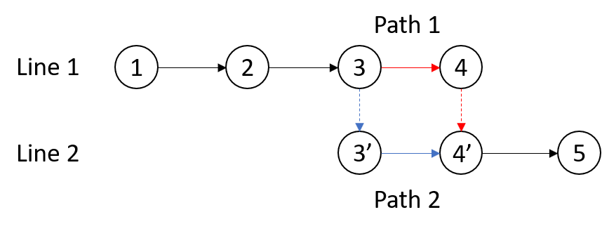
A simple example is shown below to illustrate this property. Consider the OD pairs 1-5 and 2-5 in Figure 2. There are two paths for both OD pairs. Path 1 transfers at station 4 and path 2 transfers at station 3. The path choice fractions are denoted as , respectively. Note that we ignore the time index here for simplification. Assume there are four path attributes affecting people’s choice: in-vehicle time, number of transfers and transfer walking time and commonality factor. Then we have the following proposition.
Proposition 1.
Under MNL constraints, there are and .
Proof.
Denote the utility for path of OD pair and as . Since the path 1 of OD 1-5 and the path 1 of OD 2-5 share the same transfer patterns, the number of transfers and transfer walking time for them are same. The only differences are the in-vehicle time and commonality factor. It tends out the commonality factors for these two paths are also same. The proof is easy to obtain by following Eq. (4) and is ignored here. Therefore, the utility difference for path 1 of two different OD pairs only contains in-vehicle time term. Let the total in-vehicle time for path of OD pair be . Denote the in-vehicle time for link as . and the coefficients of in-vehicle time as . We have
| (9) |
Similarly, for path 2 of OD 1-5 and OD 2-5, we have
| (10) |
According to the MNL constraint, we have
| (11) | ||||
Similarly, for path 2, we will have .
This example network is extracted and simplified from the real-world Hong Kong MTR network. Therefore, this property does hold in the real-world for many OD pairs.
∎
Besides equality constrains, there are also some inequality constraints hold under MNL constraint. For example, since all cost coefficients should be negative according our prior knowledge, if there is a path have smaller costs than other paths in the same OD pair, it should always be preferred regardless the magnitude of . So we can construct linear constraints with the form to capture this information. To automatically extract all these linear constraints in the system, we propose a Monte-Carlo sampling method. We first define a reasonable range for all (i.e. ) based on the prior knowledge (e.g. survey results from previous years), where () is the lower (upper) bound of . It is worth noting that the selection of and has very limited impact on the construction of ALC. The proof of Proposition 1 tells us the equality constraints have nothing to do with the value of . and only affects the construction of inequality constraints, and from our numerical tests the impact is very small. Generally, we only need to set the cost coefficients (e.g. in-vehicle time) to be negative.
The detailed ALC construction steps are shown in Algorithm 1. Denote the maximum number of sampling as . The choose of is a trade off between computational efficiency and constraints accuracy. Larger can help avoid the coincidence of erroneously constructing the constraints.
We denote all the constructed linear constraints for as
| (12) |
Thus, the sub-problem 1 can be reformulated as
| (13) | ||||||
Note that we replace the decision variables from to . is the prior knowledge about path share derived from . Clearly, Eq. (13) is a quadratic programming since all constraints are linear. It now can be solved very fast. However, despite Eq. (12) add some constraints to , it is not equivalent to (less strong than) the original MNL constraints. This is why we called it "approximate" linear constraints (ALC). After adding the ALC, may still have high degree of freedom. Based on the numerical test in the case study, after adding the ALC, the total degree of freedom can decrease around 40%, which demonstrates a narrower feasible space. But we still need to go one step further to make all estimated path shares satisfy the MNL constraints.
3.4.2 MNL correction
The estimated from Eq. 13 have two problems. The first is possible over-fitting due to high degree of freedom, which we have discussed before. The second is inestimable path shares due to little observed OD entry-exit flow. For example, if there is no passenger observed for OD pair in time interval . can take any values and does not affect the objective function, which makes it unable to be estimated. Both of these problems can be attributed to one reason: the estimated violates the original MNL constraints (it only satisfies the ALC of MNL).
To address this problem, we can use the estimated from Eq. (13) (called rough path shares hereafter) to obtain a set of , and then use the to generate new path shares. This procedure is called MNL correction. Path shares after MNL correction will naturally satisfy MNL constraints by definition. However, not all rough path shares are equally reliable. We have the following proposition for the reliability discussion.
Proposition 2.
The reliability of estimated from Eq. (13) is proportional to the corresponding OD entry flow .
Proof.
Intuitively, more observed passengers can provide more information for the path shares estimation. To validate it mathematically, we observe
| (14) |
by combining Eq. (1) and (2). The reliability of can be measured by the estimation variance. Thus,
| (15) |
Since is the quadratic term in the objective function of Eq. (13), analogue to the simple least square regression, we can assume for all (i.e. homoscedasticity). This leads to
| (16) |
Note that we ignore since it is constant in sub-problem 1. Recall the problem that if there is no passengers observed for a specific OD pair (), the corresponding path share is inestimable in Eq. (13). Based on our derivation in Eq. (16), this scenario results in the variance of estimated path shares equal to , which validates our derivation.
Notably, we only obtain the estimation variance of , rather than . One reason is that is hard to derive. Another is that the following estimation of based on can utilize as a whole, that is, use as the weights, which eliminates the needs for deriving .
∎
We formulate the MNL correction problem as following, which can be seen as a weighted fractional logit model [Papke and Wooldridge 1996].
| (17) |
Note that in Eq. (17), are constants. The objective function has the form of softmax function. Thus it is a convex optimization problem without constraints (like logistic regression), which can be solved efficiently. is the weight for corresponding path shares (), which reflects their reliability as we discussed in Proposition 2. After we get , the aforementioned two problems in results of Eq. (13) will naturally disappear, because we can generate a new which satisfies the MNL constraints exactly.
3.5 Discussion of solution procedures
So far, we have formulated three sub-problems to approximate the solution for the original problem. These sub-problems can be summarized in Eq. (18)-(20). In sub-problem 1(a), given the , we estimate the rough path shares, which is a quadratic programming problem. In sub-problem 1(b), given the rough path shares, we estimate the corresponding , which can be seen as a weighted fractional logit model. In sub-problem 2, given the , we load passengers to the network and return the which satisfies the NLC constraints.
- 1.
Sub-problem 1(a):
(18) - 2.
Sub-problem 1(b):
(19) - 3.
Sub-problem 2:
(20)
We expect to solve these three sub-problems iteratively and approximate the solution for the original problem. This is equivalent to find a fixed point of the following problem.
| (21) |
where SP2 is the solution function of Sub-problem 2, i.e. ; SP1a is the solution function of Sub-problem 1(a), i.e. ; SP1b is the solution function of Sub-problem 1(b), i.e. ; "" is the sign of function composition, i.e., . We are curious about the existence and uniqueness of the solution in Eq. (21), and its relationship with the original problem in Eq. (6). Before discussing the main proposition, a lemma is introduced.
Lemma 1.
If a path share set satisfies MNL constraints in terms of some choice parameters , then is the solution of sub-problem 1(b) with respect to . Mathematically, if for all , then .
Proof.
The discussion of existence of fixed point in Eq. (21) is followed. Here, we assume the objective function equal to 0 is reachable by some in the original problem (Eq. (6)), which is an ideal situation where all passengers’ behaviors are assumed to be perfectly described by the C-logit model. Extending the proof to more complicated scenarios need future works.
Proposition 3.
Proof.
Denote . Define such that for all . We claim . The proof is shown below.
Clearly, satisfies the NLC and satisfies the MNL constraints. So () is the optimal solution for the original problem. Comparing sub-problem 1(a) and the original problem, if we feed in into sub-problem 1(a), the optimal objective function of sub-problem 1(a) should be less than or equal to that of original problem because has larger feasible space in sub-problem 1(a). However, given the optimal objective function of original problem is 0, we know the optimal objective function of sub-problem 1(a) is 0 as well. And since the objective function for these two problems are same, we have is the optimal solution for sub-problem 1(a) as well.
By definition, satisfies the MNL constraints in terms of . According to Lemma 1, we have . This leads to . ∎
The proof of uniqueness requires the application of Banach fixed-point theorem [Luan and Xia 2015]. However, since has no analytical expression, it is hard to prove the uniqueness religiously. A corollary of Banach fixed-point theorem provides a way to obtain the fixed point: Start with an arbitrary and define a sequence by for . If there exists a such that . Then is the fixed point. Following this corollary, we can test the convergence of numerically based on the synthetic data described in Section 4. The results are shown in Figure 3. All has shown convergence trends despite of some slight fluctuation in the tail. The fluctuation may come from the randomness in the network loading model.


Since we validate the convergence of , the corollary of Banach fixed-point theorem can be used to develop the solution procedures. The detailed steps are summarized in Algorithm 2. To address the randomness in the network loading model, we define a "burn-in" iteration for selection, and a maximum iteration for algorithm termination (analogue to the Markov chain Monte Carlo (MCMC) methods). is the initial value of .
4 Case study and Model validation
For the purpose of model illustration and validation, we apply the proposed modeling framework on Hong Kong MTR network. The model is validated using both synthetic data and real-world AFC data.
4.1 Hong Kong MTR Network
The map for Hong Kong MTR system is shown in Fig 4. In this study, the airport express and light rail transit services are not considered since they are separated from the urban railway lines and passengers who enter the urban railway lines from these services need to tap-in again. The system consists of 10 lines and 114 stations, where 16 out of them are transfer stations. In this network, most transfer stations connect only two lines. A special case is Admiralty station in the Hong Kong island, where three lines pass through the same transfer station. The Admiralty station is in the CBD area of Hong Kong. So during peak hour there are many passengers boarding in these stations and head to the north of the city.

4.2 Validation setting
We use the AFC data on March 16th (Thursday), 2017 for the model validation. The path sets for each OD pair are provided by MTR. Li 2014 has conducted a revealed-preference (RP) route choice survey of more than 20,000 passengers in the MTR system. The estimation results are shown in Appendix A. According to Li 2014, the following attributes were used to quantify path utility: (a) total in-vehicle time, (b) number of transfer times, (c) relative walking time (total walking time divided by total route distance) and (d) the commonality factor (Eq. 4). The evening peak (18:00-19:00) is selected for validation. For simplicity, we assume the path shares are static during this hour. We set the weights in the objective function of sub-problem 1(a) as and , which means no prior knowledge is available. The maximum iteration is is set as 15 and "burn-in" iteration is set as 13. is set as 0 for all parameters. The system parameters (constants) of network loading model is summarized below. Access/Egress walking time is defined as the walking time between fare machine and train boarding platform. Warm up (cool down) time indicates the time before (after) simulation period start (end). It is needed because simulation system usually start from empty (no train and passengers). But real world does not start without train/passengers in-progress.
- 1.
Access/Egress walking time: Platform-specific, collected from MTR field measurement.
- 2.
Transfer walking time: Platform-specific, collected from MTR field measurement.
- 3.
Time table: Obtained from MTR operation team. Future research can use AVL data to get real-world train arrival and departure information.
- 4.
Capacity: 230 passengers per car according to MTR congestion standard. The number of cars for each train is obtained from MTR operation team.
- 5.
Warm up and Cool down time: 60 minutes warm up and cool down time suggested by Mo et al. 2020b.
Since the real-world path choice information usually unavailable, it is common to quantitatively validate model with synthetic data. To generate the synthetic data, we first extract the OD entry flow from the real-world AFC records. Choice parameters estimated in Li 2014 are treated as people’s "true" behavior parameters (called synthetic hereafter). Then, we use the network loading model with the true OD entry flow and the synthetic as input to simulate the travel of passengers in the system, and record people’s tap-in and tap-out time. The records of all people’s tap-in and tap-out time are treated as synthetic AFC data. For model validation, we can apply the proposed model to the synthetic AFC data and compare the estimated with the synthetic . However, in terms of real-world validation, as the ground-truth path shares are unavailable, some qualitatively analysis and indirect comparison are conducted. Details can be found in Section 4.5.
4.3 Benchmark Model
To compare the model performance, we use a purely simulation-based optimization (SBO) method [Mo et al. 2020a] as the benchmark. The formulation is shown below.
| (23a) | ||||||||
| (23b) | ||||||||
| (23c) | ||||||||
where and are the pre-determined lower and upper bound of . We set and as above. is the parameter of the network loading model, which is set equal as above. Compared with our proposed model, the purely SBO method is closer to brute-force searching. So and are usually required to narrow the feasible space and make the algorithm work. The values of and are shown in table 1. By introducing and , we actually provide the benchmark model with more information.
Many solution algorithms have been proposed to solve SBO problems. Three major classes includes direct search method, gradient-based method, and the response surface method [Osorio and Bierlaire 2013, Amaran et al. 2016]. According to Osorio and Bierlaire 2013 and Cheng et al. 2019, the response surface method is recently more popular in transportation domain and presents better performance. Thus, in this study, we adopt two response surface methods to solve the benchmark model: bayesian optimization (BYO) [Snoek et al. 2012] and constrained optimization using response surfaces (CORS) [Regis and Shoemaker 2005]. BYO aims to constructs a probabilistic model for the objective function (response surface) and then exploits this model to determine where to evaluate the objective function for next step. In each iteration the probabilistic model will be updated according to the posterior distribution. CORS also need to construct a response surface model, and update the model based on all previously probed points at each iteration. The principles for next evaluated points selection are: (a) finding new points that have lower objective function value, and (b) improving the fitting of response surface model by sampling feasible regions where little information exists. For more details regarding these two methods people can refer to Snoek et al. 2012 and Regis and Shoemaker 2005.
SBO methods are usually unstable due to the randomness in searching process. We therefore run each solution algorithm for 10 replications and show the mean and standard deviation of objective function curves. For comparison purpose, the SBO methods are only conducted in the synthetic data set because we can only compare the accuracy of path choice estimation in the synthetic data.
4.4 Results of Synthetic Data
Two indicators are reported during the iteration. One is the objective function, another is the root-mean-square-error (RMSE). The formula of RMSE is shown below.
| (24) |
where are the estimated path shares and are the synthetic path shares (unit is %). is the total number of paths in the system.
The curve of objective function is shown in Figure 5. The error bars for benchmark methods represent the standard deviation. We found the our proposed metthod can dominate the benchmark models both in convergence speed and in final convergent results. The RMSE comparison results are shown in Figure 6. We can also observe our method can approach the "true" path shares rapidly, and obtain lower estimation error than the benchmark models. Note that the RMSE may not always decrease with the reduction of objective function. This is because the relationship between path choices and OD entry-exit flows is highly non-linear.


The comparison of estimated and synthetic are shown in Table 1. The estimated of the proposed method are very close to the synthetic ones, and also outperforms the estimated from the benchmark models.
| Variable | Synthetic | Estimated | [,] | ||
| Proposed | BYO | CORS | |||
| In-vehicle time () | -0.147 | -0.156 | -0.205 | -0.231 | [-2, 0] |
| Number of transfers () | -0.573 | -0.544 | -1.218 | -1.189 | [-4, 0] |
| Relative walking time () | -1.271 | -1.291 | -2.499 | -2.316 | [-6, 0] |
| Commonality factor () | -3.679 | -3.413 | -6.184 | -6.537 | [-10, 0] |
| Objective function | - | 10328.8 | 42390.6 | 37066.1 | - |
| RMSE | - | 1.36 | 90.24 | 63.09 | - |
4.5 Results of Real-world Data
In terms of real-world data, we cannot conduct the directly comparison since the ground truth path choice is unavailable. We first conduct a qualitative analysis in terms of estimated parameters (see Table 2). Compared with the obtained by Li 2014 (i.e. the synthetic in Table 1), the scale of all coefficients are similar. The trade off between in-vehicle time and number of transfers are reasonable, where one transfer is equivalent to 7.9 minutes of in-vehicle travel time. The trade-off between in-vehicle time and walking time is relatively small for long trips but significant for short trips. The results indicate that for a trip with 4 stations (around 5 cm of map distance), one minute of transfer walking time is equivalent to 2.51 minutes of in-vehicle travel time. For a trip with 8 stations, (around 12 cm in map distance), one minute of walking time is equivalent to 1.05 minutes of in-vehicle travel time. The substitution patterns are reasonable and similar to the previous results [Li 2014].
| In-vehicle time | Number of transfers | Relative walking time | Commonality factor |
| -0.116 | -0.920 | -1.457 | -1.775 |
Though we cannot directly compare path shares, some other indicators (e.g. left behind rate) can also reflect the quality of path shares. We have the field observation data for Admiralty station Northbound platform during the testing period (18:00-19:00). The data is collected by MTR employees who counted the passengers in the platform. The average left behind rate, total number of arrival passengers (sum of tap-in and transfer passengers) and total number of boarding passengers during 18:00-19:00 are recorded. These indicators can also be obtained from network loading model which takes path shares as input. So we can input the estimated path shares into the network loading model and compare the output indicators with the ground truth. Two other path shares are used to compare with the estimated path share. One is a naive path share which assume all paths are equal likely to be chosen (named as "uniform" in Table 3). Another is the path share calculated from Li 2014, which is currently used by MTR agency for operation purpose.
The comparison results are shown in Table 3. Compared with the ground truth, the estimated path shares can generate very close number of arrival passengers and number of boarding passengers. The square error of OD entry-exit flow (i.e. the objective function) is also the lowest. Although the output left behind rate (LBR) is not as good as two baseline path shares, we observe this indicator cannot completely reflect the quality of path shares because the uniform path choice tends to generate the best LBR. But from the other three indicators we know uniform is the worst path choice among the three. Since the objective function is a network-level indicator but the other three are local platform-level, the estimated path choice is the most balanced one and gives more network-level goodness of fit, which is more suitable for the system evaluation.
| Indicators | |||||||||
| Left behind rate |
|
|
| ||||||
| Ground-truth | 0.767 | 24,945 | 24,696 | - | |||||
| Proposed model | 0.705 | 24,890 | 24,403 | 1,044,692 | |||||
| Li (2014) | 0.734 | 24,959 | 23,125 | 1,170,160 | |||||
| Uniform | 0.779 | 25,683 | 19,599 | 1,289,672 | |||||
4.6 Robustness Testing
Model robustness is an important indicator for the real-world application. In this section we test two perspectives: different initial and different case study dates. A robust model should output similar estimated regardless of initial values. In terms of different case study dates, the estimated for all weekdays in the same week should be similar since passengers’ choice behaviors are stable during a short term.
4.6.1 Different Initial
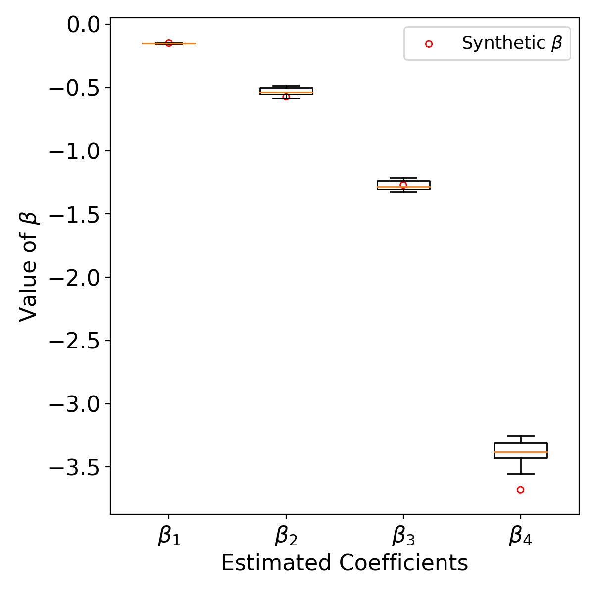
The tests of different initial are conducted in the synthetic data set because we can compare the distribution of estimated and synthetic in this way. The initial are drawn from the uniform distribution for 12 replications. Figure 7a shows the convergence of objective function with respect to different initial . The initial objective function varies a lot given different initial . But after around 10 iterations. All objective function curves converge to the same value, which demonstrates the robustness of model with respect to initial values. Figure 7b is the boxlpot of estimated of different replications. The name of ,…, can be found in Table 1. The estimated value of , and are very stable regardless of initial values. While the estimated (i.e. commonality factor) shows some fluctuations, but still within a small range (95% confidence interval is around ). This is corresponding to the survey estimation results where has a relatively low t-value (see A). It is worth noting that similar to the results in Table 1, we cannot perfectly estimate the , which leads to the synthetic located outside the 95% confidence interval. The reason may be the collinearity between commonality factor and other variables. But compared with the baseline models, our method already output a good estimate.

4.6.2 Different Case Study Dates
To test the robustness in terms of different case study dates, we applied our model to the real-world data in the week from March 13rd to March 17th, 2017. The estimated comparison is shown in Figure 8. In general, all estimated values are stable regardless of case study dates except for the coefficients of relative walking time on Friday. This may be due to that Friday night is the start of weekends, in which people have more entertainment trips in evening peak hour. And the walking time is less sensitive for entertainment trips comparing with the commuting trips. Overall, the proposed model is robust in terms of different case study weekdays in a short-term, which implies the underlying path choice behaviors of passengers is captured by the model.

5 Conclusion and Discussion
In this paper, we developed an assignment-based approach to infer the passenger route choice behavior. It models the correlation of crowding among platforms and interactions between path choice and crowding explicitly. The path choice estimation is modeled as a optimization problem. The original intractable problem is decomposed into three tractable sub-problems which can be solved efficiently. Case studies using synthetic and actual data in Hong Kong MTR system validate the effectiveness and robustness of the approach.
The advantage of this framework lies in embedding the network assignment into path choice estimation, which can incorporate the interaction between left behind and path choices. The model can be generalized to accommodate different choice model structures. For example, people can leverage path-size logit and cross nested logit model to describe to choice behaviors. The revision of the framework only requires the change of sub-problem 1(b). Moreover, more path attributes, such as waiting time, expected left-behind rate, can also be added into the consideration.
The developments in this paper have been focused on a general framework, while the models and examples we presented in this paper still have some limitations. First, we imposed the assumption on route behavior modeling that only one set of is applied for the whole network. The real-world route choice behaviour may be more diverse and heterogeneous. Future research can cluster different OD pairs with different based on the corresponding passengers’ characteristics. The model can be easily generalized with multiple sets of . Second, we assume a fixed physical capacity for the train in network loading. In the reality, the number of people can board a train may vary from stations and crowding levels [Mo et al. 2020b, Liu et al. 2016], which may also affect the path choice estimation. Future studies can incorporate the concepts of willingness to board (WtB) into the model and co-estimate the path choice, left behind and WtB.
6 Author Statement
The authors confirm contribution to the paper as follows: study conception and design: B. Mo, Z. Ma, H.N. Koutsopoulos, J. Zhao; data collection: B. Mo, Z. Ma; analysis and interpretation of results: B. Mo, Z. Ma; draft manuscript preparation: B. Mo. All authors reviewed the results and approved the final version of the manuscript.
7 Acknowledgements
The authors would like to thank Hong Kong Mass Transit Railway (MTR) for their support and data availability for this research.
References
References
- Amaran et al. [2016] Amaran, S., Sahinidis, N.V., Sharda, B., Bury, S.J., 2016. Simulation optimization: a review of algorithms and applications. Annals of Operations Research 240, 351–380.
- Atasoy et al. [2015] Atasoy, B., Ikeda, T., Song, X., Ben-Akiva, M.E., 2015. The concept and impact analysis of a flexible mobility on demand system. Transportation Research Part C: Emerging Technologies 56, 373–392.
- Cascetta et al. [1996] Cascetta, E., Nuzzolo, A., Russo, F., Vitetta, A., 1996. A modified logit route choice model overcoming path overlapping problems. specification and some calibration results for interurban networks, in: Transportation and Traffic Theory. Proceedings of The 13th International Symposium On Transportation And Traffic Theory, Lyon, France, 24-26 July 1996.
- Cheng et al. [2019] Cheng, Q., Wang, S., Liu, Z., Yuan, Y., 2019. Surrogate-based simulation optimization approach for day-to-day dynamics model calibration with real data. Transportation Research Part C: Emerging Technologies 105, 422–438.
- Davis et al. [2013] Davis, J., Gallego, G., Topaloglu, H., 2013. Assortment planning under the multinomial logit model with totally unimodular constraint structures. Work in Progress .
- Eluru et al. [2012] Eluru, N., Chakour, V., El-Geneidy, A.M., 2012. Travel mode choice and transit route choice behavior in montreal: insights from mcgill university members commute patterns. Public Transport 4, 129–149.
- Hamdouch et al. [2011] Hamdouch, Y., Ho, H., Sumalee, A., Wang, G., 2011. Schedule-based transit assignment model with vehicle capacity and seat availability. Transportation Research Part B: Methodological 45, 1805–1830.
- Hamdouch and Lawphongpanich [2008] Hamdouch, Y., Lawphongpanich, S., 2008. Schedule-based transit assignment model with travel strategies and capacity constraints. Transportation Research Part B: Methodological 42, 663–684.
- Kumar et al. [2018] Kumar, P., Khani, A., He, Q., 2018. A robust method for estimating transit passenger trajectories using automated data. Transportation Research Part C: Emerging Technologies 95, 731–747.
- Kusakabe et al. [2010] Kusakabe, T., Iryo, T., Asakura, Y., 2010. Estimation method for railway passengers’ train choice behavior with smart card transaction data. Transportation 37, 731–749.
- Lam and Xie [2002] Lam, S.H., Xie, F., 2002. Transit path-choice models that use revealed preference and stated preference data. Transportation Research Record 1799, 58–65.
- Li [2014] Li, W., 2014. Route and transfer station choice modeling in the MTR system. Working paper.
- Liu et al. [2016] Liu, Z., Wang, S., Chen, W., Zheng, Y., 2016. Willingness to board: a novel concept for modeling queuing up passengers. Transportation Research Part B: Methodological 90, 70–82.
- Luan and Xia [2015] Luan, H., Xia, Z., 2015. Theorem of existence and uniqueness of fixed points of monotone operators, in: Genetic and Evolutionary Computing. Springer, pp. 11–17.
- Mo et al. [2020a] Mo, B., Ma, Z., Koutsopoulos, H., Zhao, J., 2020a. Calibrating route choice for urban rail system: A comparative analysis using simulation-based optimization methods, Transportation Research Board 99th Annual Meeting.
- Mo et al. [2020b] Mo, B., Ma, Z., Koutsopoulos, H., Zhao, J., 2020b. Network performance model for urban rail systems. Transportation Research Record. Forthcoming.
- Nazem et al. [2011] Nazem, M., Trépanier, M., Morency, C., 2011. Demographic analysis of route choice for public transit. Transportation Research Record 2217, 71–78.
- Nguyen et al. [2001] Nguyen, S., Pallottino, S., Malucelli, F., 2001. A modeling framework for passenger assignment on a transport network with timetables. Transportation Science 35, 238–249.
- Osorio and Bierlaire [2013] Osorio, C., Bierlaire, M., 2013. A simulation-based optimization framework for urban transportation problems. Operations Research 61, 1333–1345.
- Papke and Wooldridge [1996] Papke, L.E., Wooldridge, J.M., 1996. Econometric methods for fractional response variables with an application to 401 (k) plan participation rates. Journal of applied econometrics 11, 619–632.
- Prato [2009] Prato, C.G., 2009. Route choice modeling: past, present and future research directions. Journal of choice modelling 2, 65–100.
- Regis and Shoemaker [2005] Regis, R.G., Shoemaker, C.A., 2005. Constrained global optimization of expensive black box functions using radial basis functions. Journal of Global optimization 31, 153–171.
- Snoek et al. [2012] Snoek, J., Larochelle, H., Adams, R.P., 2012. Practical bayesian optimization of machine learning algorithms, in: Advances in neural information processing systems, pp. 2951–2959.
- Song et al. [2017] Song, W., Han, K., Wang, Y., Friesz, T., Del Castillo, E., 2017. Statistical metamodeling of dynamic network loading. Transportation research procedia 23, 263–282.
- Sun et al. [2015] Sun, L., Lu, Y., Jin, J.G., Lee, D.H., Axhausen, K.W., 2015. An integrated bayesian approach for passenger flow assignment in metro networks. Transportation Research Part C: Emerging Technologies 52, 116–131.
- Sun and Xu [2012] Sun, Y., Xu, R., 2012. Rail transit travel time reliability and estimation of passenger route choice behavior: Analysis using automatic fare collection data. Transportation Research Record 2275, 58–67.
- Xu et al. [2018] Xu, X., Xie, L., Li, H., Qin, L., 2018. Learning the route choice behavior of subway passengers from afc data. Expert Systems with Applications 95, 324–332.
- Zhao et al. [2017] Zhao, J., Zhang, F., Tu, L., Xu, C., Shen, D., Tian, C., Li, X.Y., Li, Z., 2017. Estimation of passenger route choice pattern using smart card data for complex metro systems. IEEE Transactions on Intelligent Transportation Systems 18, 790–801.
- Zhou and Xu [2012] Zhou, F., Xu, R.h., 2012. Model of passenger flow assignment for urban rail transit based on entry and exit time constraints. Transportation Research Record 2284, 57–61.
- Zhu [2017] Zhu, Y., 2017. Passenger-to-itinerary assignment model based on automated data. Ph.D. thesis. Northeastern University.
Appendix A Passenger Route Choice Model for MTR System
These results are from Li 2014. The C-logit Model formulation is same to Eq. (3) and Eq. (4). A total number of 31,640 passengers completed the questionnaire. After filtering duplicate responses, 26,996 responses were available. The model results are shown in Table 4. The main explanatory variables are the total in-vehicle time, relative transfer walking time and number of transfers. All variables are statistically significant with the expected signs. Routes with high in-vehicle time, walking time and number of transfers are less likely to be chosen by passengers.
| Estimate | Std. Error | t-value | ||
| In-vehicle time | -0.147 | 0.011 | -13.64 | *** |
| Relative walking time | -1.271 | 0.278 | -4.56 | *** |
| Number of transfers | -0.573 | 0.084 | -6.18 | *** |
| Commonality factor | -3.679 | 1.273 | -2.89 | ** |
| ***: ; **: . | ||||