Don’t Judge an Object by Its Context: Learning to Overcome Contextual Bias
Abstract
Existing models often leverage co-occurrences between objects and their context to improve recognition accuracy. However, strongly relying on context risks a model’s generalizability, especially when typical co-occurrence patterns are absent. This work focuses on addressing such contextual biases to improve the robustness of the learnt feature representations. Our goal is to accurately recognize a category in the absence of its context, without compromising on performance when it co-occurs with context. Our key idea is to decorrelate feature representations of a category from its co-occurring context. We achieve this by learning a feature subspace that explicitly represents categories occurring in the absence of context along side a joint feature subspace that represents both categories and context. Our very simple yet effective method is extensible to two multi-label tasks – object and attribute classification. On challenging datasets, we demonstrate the effectiveness of our method in reducing contextual bias.
1 Introduction
Visual context serves as a valuable auxiliary cue for the human visual system for scene interpretation and object recognition biederman1982scene. Context can either be a co-occurrence of objects and scenes (e.g., “boat” is often present in “outdoor waters”) or of two or more objects in a given scene (e.g., “skis” often co-occur with a “skier”). Context becomes especially crucial for our visual system when the visual signal is ambiguous or incomplete (e.g., due to occlusion, viewpoint of the scene capture, etc.). Past research explicitly models context and shows benefits on standard visual tasks such as classification tang-cvpr15 and detection divvala-cvpr09; barnea-cvpr19. Meanwhile, convolution networks by design implicitly capture context.

Deep networks rely on the availability of large-scale annotated datasets lin-eccv14; deng_cvpr09 for training. As highlighted in torralba-cvpr11; tommasi-2017, despite the best efforts of its creators, most prominent vision datasets are afflicted with several forms of biases. Let us consider an object category “microwave.” A significant portion of images belonging to this category are likely to be captured in kitchen environments, where other objects such as “refrigerator,” “kitchen sink,” and “oven” frequently co-occur. This may inadvertently induce contextual bias in these datasets, which would consequently seep into models trained on them. Specifically, in the process of learning features that separate positive and negative instances in such a (biased) training dataset, a deep discriminative model can very often also strongly capture the context co-occurring with the category of interest. This issue is exacerbated in a setting where we do not have explicit location annotations (e.g., bounding boxes and segmentation masks) of such biased categories, and a model being trained has to rely solely on image-level annotations to perform multi-label classification. Having a model implicitly learn to localize such context-biased categories in the absence of location annotations is challenging.
Does it even matter if a model inadvertently learns such correlations? We believe this can cause problems on two fronts: (1) failing to identify “microwave” in a different context such as an “outdoor” scene or in the absence of “refrigerator” and (2) hallucinating “refrigerator” even in an indoor kitchen scene containing only “microwave.” The issue of co-occurring bias is also prevalent in visual attributes liu-cvpr16; xian-tpami18. For example, in the Deep Fashion dataset liu-cvpr16, the attribute “trapeze” strongly co-occurs with “striped.” This results in a less credible classifier that has a hard time recognizing “trapeze” in clothes with “floral.” Recent research has identified far more serious mistakes made by trained models due to inherent biases in both language and vision datasets – learning correlations between ethnicity and certain sport activities stock2018convnets, gender and profession bolukbasi2016man; hendricks2018women; zhao2017men, and age and gender of celebrities alvi-eccv18. Such grave confusion caused due to biases in the data impedes the deployment of these models in real-world applications.
Given these issues, our goal is to train an unbiased visual classifier that can accurately recognize a category both in the presence and absence of its context. Specifically, given two categories with a strong co-occurring bias, our aim is to accurately recognize them when either one occurs exclusively, and at the same time not hurt the performance when they co-occur. To this end, we propose two key ideas. First, we hypothesize that a network should learn about a category by relying more on its corresponding pixel regions than those of its context. Since we only have class labels, we use class activation maps (CAM) zhou-cvpr16 as “weak” location annotations and minimize their mutual spatial overlap.
Building on this, we devise a second method that learns feature representations to decorrelate a category from its context. While the entire feature space learned by the network jointly represents category and context, we explicitly carve out a subspace to represent categories that occur away from typical context. We learn this feature subspace only from training instances where a biased category occurs in the absence of its context. In all other cases, the model should also leverage context and thus the entire feature space. At test time, we make no such distinction and the entire feature space is equally leveraged. Therefore, in the example from Fig. 1, our goal is to learn a feature subspace to represent “skateboard” while the entire feature space jointly represents “skateboard” and “person.”
Through extensive evaluation, we demonstrate significant performance gains for the hard cases where a category occurs away from its typical context. Crucially, we show that our framework does not adversely effect recognition performance when categories and context co-occur. To summarize, we make the following contributions:
- •
With an aim to teach the network to “learn from the right thing,” we propose a method that minimizes the overlap between the class activation maps (CAM) of the co-occurring categories (Sec. 4.1).
- •
Building on the insights from the CAM-based method, we propose a second method that learns feature representations that decorrelate context from category (Sec. 4.2).
- •
We apply both methods on two tasks: object and attribute classification, and datasets, and achieve significant boosts over strong baselines for the hard cases where a category occurs away from its typical context (Sec. 5).
2 Related work
Addressing biases: Prior work torralba-cvpr11; khosla-eccv12; van-arxiv16; tommasi-2017 has shown that existing datasets suffer from bias and are not perfectly representative of the real world. Hence, a model trained on such data will have difficulty generalizing to non-biased cases. Attempts to reduce dataset bias include domain adaptation techniques csurka-arxiv17 and data re-sampling chawla2002smote; li-cvpr19, e.g., so that minority class instances are better represented. One limitation of data re-sampling is that it can involve reducing the dataset, leading to sub-optimal models. Recent adversarial learning approaches alvi-eccv18; kim-cvpr19 try to mitigate bias from the learned feature representations while optimizing performance for the task at hand (e.g., removing gender bias while classifying age). However, these methods would not be directly applicable for mitigating contextual bias, as context (the bias factor) can still be useful for recognition—so it cannot be simply removed. Others study various forms of bias in the context of image captioning (e.g., gender bias) hendricks2018women, image classification (e.g., ethnicity bias) stock2018convnets, and object recognition (e.g., socio-economic bias) vries-cvprw19. Overall, contextual bias in visual recognition remains relatively under explored.
Co-occurring-bias: Contextual bias is a well-studied problem in the field of natural language processing recasens-acl13; sun-arxiv19, however, it is much less studied in the computer vision community. In vision, most efforts consider context as a useful cue divvala-cvpr09; barnea-cvpr19. A few efforts have shown that a recognition model will fail to recognize an object without its co-occurring context, but do not propose a solution choi-prl12; rosenfeld-arxiv18.
A recent method reduces contextual bias in video action recognition wang-cvpr18, but it relies on temporal information and thus cannot be applied to the image recognition problems we tackle in this work. A pre-deep learning approach jayaraman-cvpr14 reduces the correlation (bias) between visual attributes by leveraging additional knowledge in the form of semantic groupings of attributes. Recently zhu-cvpr19 tried to reduce contextual bias for object detection by learning focused foreground features, but they require expensive bounding-box annotations. In contrast, our deep learning approach does not require any additional supervision apart from the object/attribute class labels. Most importantly, to our knowledge, there is no prior work focusing on mitigating contextual bias for object classification as we do in this paper.
Relation to few-shot learning:
Lastly, contextual bias could also be formulated as a few-shot snell-nips2017; karlinsky-cvpr19; alfassy-cvpr19 or class imbalance elkanfoundations; cui-cvpr19 problem, since images in which objects appear without their usual co-occurring context (e.g., keyboard without a mouse next to it) are relatively rare. However, treating such rare (exclusive) images as a separate class or simply assigning them higher weight can be sub-optimal, as we show in our experiments.
3 Problem setup
Our method operates on the premise that the training data distribution corresponding to a few categories suffers from co-occurring bias. We henceforth refer to them as biased categories. We make no such assumptions about the test data distribution. For example, COCO-Stuff caesar-cvpr18 has images where “ski” co-occurs with “person,” but only has images where “ski” occurs without “person.” A model trained on such skewed data may fail to recognize when “ski” occurs in isolation. Our goal is to learn a feature space that is robust to such training data biases. In particular, given a (presumably) unbiased test dataset, our goal is to (1) correctly identify “ski” when it occurs in isolation and (2) not lose performance when “ski” co-occurs with “person.” A key aspect of our approach is to identify most biased categories for a given dataset, which we describe next.
3.1 Identifying biased categories
Suppose we are learning a classifier on a multi-label training dataset with a vocabulary of categories. Only a few of these categories suffer from context11
1
Throughout, we use context and co-occurring interchangeably. bias; thus, a key aspect of our approach is to find this set of category pairs , , where , which suffer the most from co-occurring bias22
2
Although we consider pairs of co-occurring categories throughout, the proposed method is extensible for any number of co-occurring categories.. Henceforth, (e.g. “ski”) denotes a class which is most biased with (e.g. “person”) due to its high co-occurrence.
Intuition: While there are several ways to construct , our method is built on the following intuition: a given category is most biased by if (1) the prediction probability of drops significantly in the absence of and (2) co-occurs frequently with .
We now define our method to identify for a given . For a given category , let and denote sets of images where occurs with and without respectively. Let denote the prediction probability of an image for a category obtained from training a standard multi-label classifier. We quantify the extent of between and as follows:
| (1) |
where denotes cardinality of a set. Eq (1) measures the ratio of average prediction probabilities of the category when it occurs with and without (see Fig. 2). A higher value indicates a higher dependency of on . We determine as follows:
| (2) |
i.e., for each , we identify a category that (i) yields the highest value of and (ii) co-occurs at least times (see Sec. 4.3) with . We then construct with most biased category pairs. We note that the above formulation is directional, i.e., it only captures the biases in caused due to . For instance, only captures bias in “ski” due to “person” but not vice-versa.
We next propose two methods to combat co-occurring bias in the training data. The input to both methods is (1) training images and their associated weak (multiple) category labels and (2) the set composed of the most biased category pairs (identified from Eq. (1)). We stress that training images have only weak labels stating which categories are present; they have no spatial annotations to say where in the image each category is.
4 Approach
Our first method relies on class activation maps (CAM) as “weak” automatically inferred location annotations and minimizes their spatial overlap between biased categories (Sec. 4.1). Building on the observations from this CAM-based approach, we propose a second method which learns a feature space by encouraging context sharing when a biased category co-occurs with context while suppressing context when it occurs in isolation (Sec. 4.2).
4.1 CAM as “weak” location annotation

Our method operates on the following premise: as almost always co-occurs with , the network may learn to inadvertently rely on pixels corresponding to to predict . This is particularly problematic when the network is tested on images where occurs in the absence of . We hypothesize that one way to overcome this issue is to explicitly force the network to rely less on ’s pixel regions, without using location annotations. While this may not succeed for occluding pairs like “person” and “shirt,” it seems like a natural constraint for spatially-distinct categories like “person” and “skateboard.”
Class Activation Maps: To this end, we propose to use class activation maps (CAM) zhou-cvpr16 as a proxy for object localization information. For a given image and class , indicates the discriminative image regions used by a deep network to identify . Specifically, the final convolutional layer () of any typical network is followed by a global pooling and a fully connected () layer which predicts a score for class in image . is generated by projecting back the
weights of the layer for on and computing a weighted average of the feature maps. Though CAMs are typically used as a visualization technique, in this work, we also use them to reduce contextual bias as we describe next.
Formulation:
In our setup, for each biased category pair in (defined in Sec. 3.1), we enforce minimal overlap of their CAMs via the loss function:
| (3) |
CAM offers two nice properties: (1) it is learned only through class labels without requiring any annotation effort and (2) it is fully differentiable, and thus can be integrated in an end-to-end network during training.
Ideally, Eq (3) should learn to reduce the spatial overlap between co-occurring categories, without hurting the classification performance. However, while attempting to minimize overlap, Eq (3) could also lead to a trivial solution where the CAMs of and drift apart from their actual pixel regions. To prevent this without strongly-supervised spatial annotations, we introduce a regularization term . Specifically, we pre-train a separate network (offline) for the standard classification task and generate from it for and . We then ground the CAMs of each category to be closer to its pixel regions predicted from . is thus defined as follows:
| (4) |
We use a standard binary cross-entropy loss () for the task of multi-label classification. Thus, our final loss becomes:
| (5) |
Fig. 3 for the entire approach. As we show in results (Sec. 5), our CAM-based method successfully learns to rely more on the biased category’s pixel regions thereby improving recognition performance. Our method yields large gains when a biased category occurs in the absence of its typical context. However, it sometimes hurts performance when biased category co-occurs with context (discussed later in Fig. 7). One reason could be that the pixel regions surrounding the co-occurring category also offer useful complementary information for recognizing the biased category. By discouraging mutual spatial overlap, CAM-based approach may not be able to leverage this information. This key insight led to the formulation of our next approach, which splits the feature space into two and separately represents context and category, while posing no constraints on their spatial extents.
4.2 Feature splitting and selective context suppression

Rather than optimizing CAMs, we propose to learn a feature space that is robust to the inherent co-occurring biases in the training data. We observe that cases when a biased category co-occurs with context are often visually distinct from those where it occurs exclusively (see Fig. 1). This motivates us to learn a dedicated feature (sub) space to represent biased categories occurring away from their typical context. While the entire feature space learned by the model jointly represents context and category, this dedicated subspace should decouple the representations of a category from its context. We learn this feature subspace only from training instances where biased categories occur in the absence of their typical context. These modifications only affect training; at inference time the architecture is identical to the standard model.
Formulation: Given a deep neural network , let denote the -dimensional output of the final pooling layer just before the fully-connected layer (). Let the weight matrix associated with layer be , where denotes the number of categories in a given multi-label dataset. The predicted scores inferred by a classifier (ignoring the bias term) are
| (6) |
Because we wish to separate the feature representations of a category from its context, we (row-wise) split randomly into two disjoint subsets: and , each of dimension . Consequently, is split into and and the above equation can be rewritten as:
| (7) |
In scenarios where a biased category occurs in the absence of its context, we want to enforce the network to only rely on by suppressing . This step allows the network to explicitly capture the biased category-specific information when it occurs away from its context in . On the other hand, when a biased category co-occurs with its context, we want to encourage the network to leverage both and . This would allow the network to jointly encode category and context in the full feature space.
To achieve this, we make two minor modifications to a standard classifier when a biased category occurs away from its typical context. First, we disable back propagation through thereby forcing the network to learn only through . Second, we set to a constant value. We believe these two simple modifications allow us to suppress context in selective cases, i.e., when a biased category occurs away from its context. For instance, when ski occurs in the absence of its typical context person, our method suppresses thereby encouraging to encode its appearance; when ski co-occurs with person, both and are leveraged.
In practice, we set , where is the average of over the last mini-batches, and allowed stabler training. Also, is a closer approximation to the range of values witnesses at test time.
Intuition behind weighted loss: An underlying aspect of our method is that the biased categories occur very rarely in the absence of their context, making the training data distribution skewed (see Sec. 3). This is a problem since is learned solely from the (very few) samples with biased categories occurring in the absence of their typical context. We address this issue by associating a higher weight to such training samples. All other samples are weighed equally. Specifically, we define a weight such that
| (8) |
Thus, is the ratio of the number of training instances where category occurs in the presence vs. absence of context. A higher value of for a given biased category indicates more data skewness. 33 3 In practice, we ensure is at least (a constant value ) when occurs exclusively..
Given ground-truth label and sigmoid function , our weighted binary cross-entropy loss is defined as follows:
| (9) |
Figure 4 illustrates the proposed method. While a standard classifier jointly encodes category and context, it fails to recognize biased categories occurring without context. By contrast, our approach splits the feature space and represents biased categories occurring without context in a dedicated subspace. As we will show in results, due to selective context suppression, this feature subspace successfully captures category-specific information. Furthermore, in the second subspace, our method effectively leverages context when available and jointly encodes it with category.
As we show in results, leveraging context when available, distinguishes this method with the CAM-based method described in Sec. 4.1 and plays a key role in recognition performance. Further, while we selectively suppress context when a biased category occurs away from its context, the CAM-based method optimizes the mutual spatial overlap when a biased category co-occurs with context. We stress that both methods are applied only for the biased category pairs; thus, misclassification loss for the other (non-biased) categories also plays an important role in learning. Finally, our method poses no constraints on the spatial extents of categories; thus, unlike our CAM-based approach, is extensible to attributes.
4.3 Training setup
Determining biased categories: For each category, we first identify other categories that occur frequently (at least times, based on the dataset). Next, we partition the training data into non-overlapping split. We train a standard multi-class classifier with BCE loss on the split and compute (Eq. 1) on the split. While both methods proposed in this work can be applied to any number of biased category pairs, we found that setting (Sec. 3.1) sufficiently captures biased categories in all the datasets we study here.
Optimization: We follow a two-stage training procedure: in the first stage, we start with a pre-trained network as a backbone and fine-tune it on all categories of a given dataset. This step ensures that the network learns useful context cues for the target task. In the second stage, we fine-tune our network and separately apply the modified loss defined in each proposed method. In the CAM-based approach, we reduce spatial overlap between the category pairs; in the feature splitting method, we selectively suppresses context when the biased categories occur exclusively and encourage context sharing in all other scenarios.
Implementation details: For both proposed methods, we use ResNet-50 he-cvpr16 pre-trained on ImageNet as a backbone. For the first stage, an initial learning rate of is used which is later divided by following the standard step decay process for the learning rate. Following this, during the second stage of training, we train the network with a learning rate of for both methods. For the CAM-based approach, we set and to be and respectively.
The input images are randomly resize crop to during the training. To further augment training data, we horizontal flip images. We use a batch size of and stochastic gradient descent for optimization. Our model is implemented using PyTorch 1.0. Overall training time of both proposed methods is very close to that of a standard classifier and their inference time is exactly same as that of the standard classifier.
5 Experiments
In this section, we study the effectiveness of our approach across two tasks: object and attribute classification. We first describe our evaluation setup then report qualitative and quantitative performance on four image datasets against competitive baselines.
| Datasets | Task | #Classes | #Train / #Test |
|---|---|---|---|
| MS COCO + Stuff caesar-cvpr18 | object | 171 | 82,783 / 40,504 |
| UnRel peyre-iccv17 | object | 43 | - / 1,071 |
| Deep Fashion liu-cvpr16 | attribute | 250 | 209,222/40,000 |
| AwA xian-tpami18 | attribute | 85 | 30,337 / 6,985 |
Datasets:
We evaluate our approach on four multi-label datasets (summarized in Table 1). The choice of these datasets was driven by the fact that they exhibit strong co-occurrence bias. We summarize their co-occurrence statistics in the supplementary material. For DeepFashion liu-cvpr16, we only consider most frequent attributes in the training data as other attributes do not have sufficient training samples. For Animals with Attributes (AwA) jayaraman-cvpr14; xian-tpami18, following common practice, we train an attribute prediction network on seen () animal categories and evaluate on unseen () categories. Finally, UnRel dataset peyre-iccv17 contains images of objects in unusual contexts, as they are obtained from rare and unusual triplet queries (e.g. “person ride giraffe,” “dog ride bike”). We stress-test the generalizability of our model pre-trained on COCO-Stuff on this dataset.
Evaluation setup:
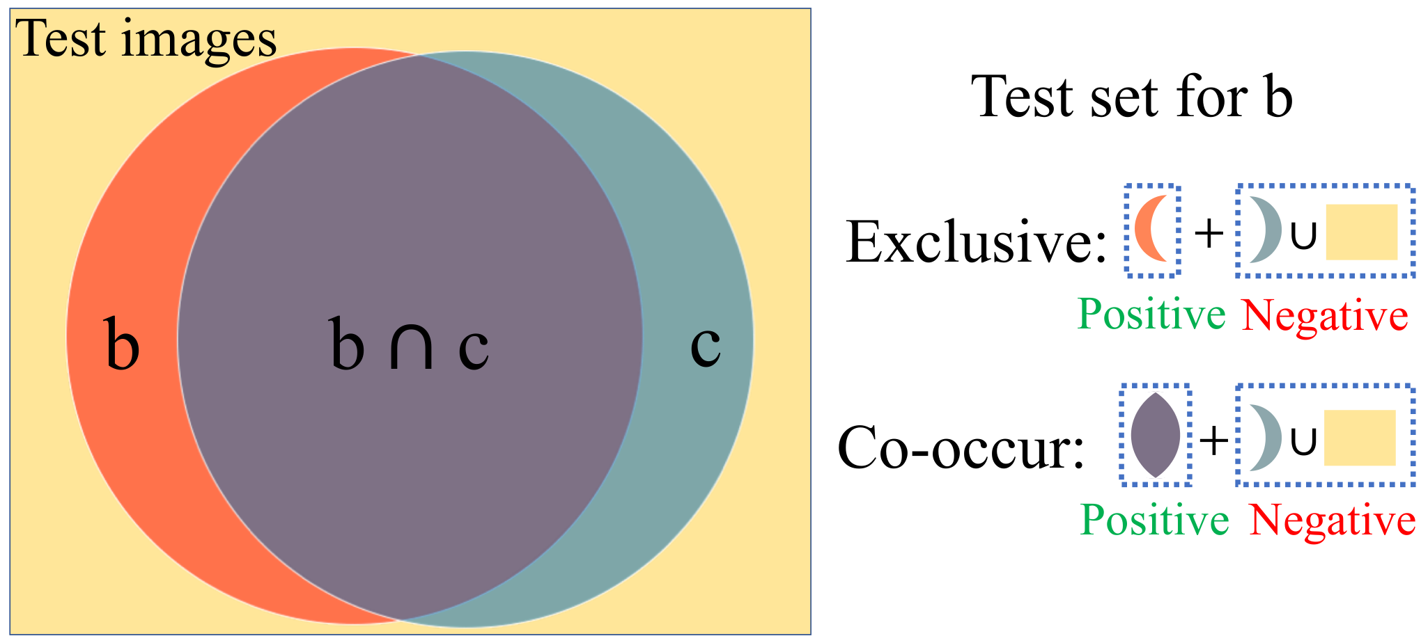
We reiterate that our goal is to improve performance when highly biased categories occur exclusively, without losing much performance when they co-occur with other categories. Towards this end, for each dataset, we first determine the most biased category pairs () following the approach in Sec. 3.1. Next, for these category pairs, we report performance on two different test data distributions: (1) exclusive: never occurs with and (2) co-occur: always co-occurs with . We illustrate the two test distributions in Fig. 5. We report top-3 recall for DeepFashion liu-cvpr16 and mAP for all other datasets.
Baselines:
Aside from a standard classifier trained with a binary cross-entropy loss for each category, we compare with the following state-of-the-art methods that tackle the issue of co-occurring bias: (1) class balancing loss cui-cvpr19 by treating the scenarios where biased categories occur exclusively as tail classes and (2) attribute decorrelation approach jayaraman-cvpr14, where we replace the hand-crafted features with deep network features (conv5 features of ResNet-50) for a fairer comparison. To further test the strength of our method, we designed the following competitive baselines:
- 1.
remove co-occur labels, where we remove labels corresponding to for each in during training. By removing supervision about co-occurring categories, we intend to soften the context-induced bias on the model.
- 2.
remove co-occur images shares the same motivation as (2) but instead we remove training instances where the biased category and context co-occur.
- 3.
weighted loss, where we apply times higher weight to the loss when biased categories occur exclusively.
- 4.
negative penalty, where we assign a large negative penalty if the network predicts co-occurring category in cases where a biased category occurs exclusively.
| Methods | Exclusive | Co-occur |
|---|---|---|
| standard | 24.5 | 66.2 |
| class balancing loss cui-cvpr19 | 25.0 | 66.1 |
| remove co-occur labels | 25.2 | 65.9 |
| remove co-occur images | 28.4 | 28.7 |
| weighted loss | 30.4 | 60.8 |
| negative penalty | 23.8 | 66.1 |
| ours-CAM | 26.4 | 64.9 |
| ours-feature-split | 28.8 | 66.0 |
5.1 Object Classification Performance
5.1.1 Overall Results
In Table 2, we report performance on COCO-Stuff for the most biased categories. First, we observe that the standard classifier has much better performance for co-occurring compared to exclusive test splits. This clearly demonstrates the inherent contextual bias present in COCO-Stuff, as standard classifier struggles when biased categories do not co-occur with context. class balancing loss yields marginal gains indicating that weighing the rare exclusive cases alone cannot address contextual bias.
Next, we observe that both ours-CAM and ours-feature-split outperform standard by and respectively on the exclusive test set. ours-feature-split has a very marginal drop of on the co-occurring split, compared to standard, while the performance drop is higher for ours-CAM. On categories such as “ski” and “skateboard” which have a very high co-occurrence bias with “person”, the mAP boost from ours-feature-split is and respectively (per-class mAP for both methods in supp. material).
Comparison with other baselines: We note that remove co-occur images approach performs poorly as it relies only on the exclusive images of the biased categories and do not take advantage of the vast amount of co-occurring images which supply complementary visual information. weighted loss improves performance on the exclusive test split compared to ours-feature-split (30.4% vs. 28.8%), but significantly hurts performance on co-occurring split (60.8% vs. 66.0%). negative penalty does not hurt co-occurring split, but has inferior performance compared to our methods on the exclusive split. We also note that performance trends exhibited by these methods are consistent across all other datasets we test on; for all future experiments, we compare our methods with standard and class balancing loss.
Performance on the non-biased categories: We evaluate on the non-biased object categories of COCO-Stuff and observe that both ours-CAM and ours-feature-split perform on par with standard, with a very mild drop of overall mAP (details in supp. material). This indicates that our methods, while successfully improving performance for the biased categories, do not adversely effect the rest of the (non-biased) categories.


5.1.2 Qualitative Analysis
Next, we use CAM as a visualizing tool to analyze how our methods effectively tackle contextual bias.
standard vs. ours-CAM: In Fig. 6, we present evidence where standard fails but ours-CAM succeeds44
4
We determine ‘success’ when the predicted probability is and ‘failure’ otherwise. to recognize biased categories.
In both cases where a biased category co-occurs with context as well as occurs in its absence, ours-CAM focuses on the right category thus “learns from the right thing.”
ours-CAM vs. ours-feature-split:
Fig. 7 presents cases where ours-feature-split succeeds but ours-CAM struggles to recognize biased categories. We observe that while ours-CAM rightly focuses on the category’s pixel regions, ours-feature-split additionally leverages the available context and thus performs better.
standard vs. ours-feature-split:
The first columns in Fig. 8 present evidence where the standard classifier fails but ours-feature-split succeeds. For example, our method is able to recognize “skateboard” and “snowboard” in the absence of “person”, and “microwave” in the absence of “oven”. By contrast, the standard classifier relies more on the context, thus fails on these images. The last column presents some failure cases where both ours-feature-split and standard fail when biased categories occur without context. Common failure cases are challenging scenarios when the image has poor lighting, the object is zoomed out and thus very small (e.g., microwave).
Analysing and :
Recall that in Sec. 4.2, ours-feature-split is formulated with a goal to prominently capture biased category-specific features through and context through . We visually verify this by generating two distinct class activation maps:
(i) weighted by and (ii) weighted by . From Fig. 9, it is evident that learns to prominently focus on the category (e.g., handbag, car) and on the co-occurring context (e.g., person, road).

| Methods | standard | ours-CAM | ours-feature-split |
| mAP | 42.0 | 45.3 | 52.1 |
5.2 Cross dataset experiment on UnRel
We next perform a cross-dataset experiment by taking our models trained on COCO-Stuff and testing them directly — without any fine-tuning — on UnRel dataset. UnRel has objects that are out-of-context (e.g., cat on a skateboard). Thus, a model that truly understands what the object is would be able to correctly classify it compared to a model that relies heavily on (or confuses the object with) context. Thus, this setting is a great testbed to evaluate our methods. Because we do not finetune, we evaluate only on the categories of UnRel that overlap with the biased categories of COCO-Stuff. From Table 3, we observe that both ours-CAM and ours-feature-split outperform standard by a large margins. This clearly demonstrates that both our methods learn from the right category and overcome contextual bias.
5.3 Attribute Classification
|
| |||||||
|---|---|---|---|---|---|---|---|---|
| Methods | Exclusive | Co-occur | Exclusive | Co-occur | ||||
| standard | 4.9 | 17.8 | 19.4 | 72.2 | ||||
| class balancing loss cui-cvpr19 | 5.2 | 19.4 | 20.4 | 68.4 | ||||
| attribute decorrelation jayaraman-cvpr14 | - | - | 18.4 | 70.2 | ||||
| ours-feature-split | 9.2 | 20.1 | 20.8 | 72.8 | ||||
Here, we show that our approach of reducing contextual bias generalizes to attributes. Our CAM-based approach is not applicable to attributes, as they lack well-defined spatial extents (details in Sec. 4.1). As noted in Sec 5.1, the inherent contextual bias and difficulty in recognizing biased categories in the absence of their context leads to low scores on exclusive test split for all methods and datasets.
Results on DeepFashion: As is the common practice, we report per class top- recall on DeepFashion liu-cvpr16. From Table 4, we note that ours-feature-split outperforms standard by a significant margin on both test splits. For attributes like trapeze and bell which exhibit strong co-occurrence with striped and lace respectively, ours-feature-split yields a boost of and top-3 recall respectively compared to standard classifier. We present per-attribute results and comparisons with other baselines in the suppl. material.
Results on Animals with Attributes: Animals with Attributes xian-tpami18 suffers from severe bias among attributes, e.g. blue and spots are highly correlated to coastal and long leg respectively. In this task, the goal is to learn an attribute classifier on “seen” animal categories (e.g “spots” attribute from the animal category “dalmatian”) and evaluate the model’s generalizability on unseen animal categories (e.g. “spots” attribute on the unseen animal category “leopard”). From Table 4, we observe that ours-feature-split offers gains on the exclusive test split over other methods without hurting the co-occurring case. In particular, we outperform attribute decorrelation jayaraman-cvpr14, which was specifically designed to decorrelate attributes.
6 Conclusion
We demonstrated the problem of contextual bias in popular object and attribute datasets by showing that standard classifiers perform poorly when biased categories occur away from their typical context. To tackle this issue, we proposed two simple yet effective methods to decorrelate feature representations of a biased category from its context. Both methods perform better at recognizing biased classes occurring away from their co-occurring context while maintaining the overall performance. More importantly, our methods generalize to new unseen datasets and perform significantly better than standard methods. Our current framework tackles contextual bias between pairs of categories; future efforts should leverage more available (scene or category) information and model relationships between them. Extending proposed methods to tasks like object detection and video action recognition is a worthy future direction.
Acknowledgments.
This work was supported in part by NSF CAREER IIS-1751206.
References
- (1) Amit Alfassy, Leonid Karlinsky, Amit Aides, Joseph Shtok, Sivan Harary, Rogerio Feris, Raja Giryes, and Alex M Bronstein. Laso: Label-set operations networks for multi-label few-shot learning. In CVPR, 2019.
- (2) Mohsan Alvi, Andrew Zisserman, and Christoffer Nellåker. Turning a blind eye: Explicit removal of biases and variation from deep neural network embeddings. In ECCV, 2018.
- (3) Ehud Barnea and Ohad Ben-Shahar. Exploring the bounds of the utility of context for object detection. CVPR, 2019.
- (4) Irving Biederman, Robert J. Mezzanotte, and Jan C. Rabinowitz. Scene perception: Detecting and judging objects undergoing relational violations. Cognitive psychology, 1982.
- (5) Tolga Bolukbasi, Kai-Wei Chang, James Y Zou, Venkatesh Saligrama, and Adam T Kalai. Man is to computer programmer as woman is to homemaker? debiasing word embeddings. In NIPS, 2016.
- (6) Holger Caesar, Jasper Uijlings, and Vittorio Ferrari. Coco-stuff: Thing and stuff classes in context. In CVPR, 2018.
- (7) Nitesh Chawla, Kevin Bowyer, Lawrence Hall, and Philip Kegelmeyer. Smote: synthetic minority oversampling technique. JAIR, 2002.
- (8) Myung Jin Choi, Antonio Torralba, and Alan S Willsky. Context models and out-of-context objects. Pattern Recognition Letters, 2012.
- (9) Gabriela Csurka. Domain adaptation for visual applications: A comprehensive survey. arXiv preprint arXiv:1702.05374, 2017.
- (10) Yin Cui, Menglin Jia, Tsung-Yi Lin, Yang Song, and Serge Belongie. Class-balanced loss based on effective number of samples. In CVPR, 2019.
- (11) Terrance de Vries, Ishan Misra, Changhan Wang, and Laurens van der Maaten. Does object recognition work for everyone? In CVPRW, 2019.
- (12) Jia Deng, Wei Dong, Richard Socher, Li-Jia Li, Kai Li, and Li Fei-Fei. ImageNet: A Large-Scale Hierarchical Image Database. In CVPR, 2009.
- (13) Santosh K Divvala, Derek Hoiem, James H Hays, Alexei A Efros, and Martial Hebert. An empirical study of context in object detection. In CVPR, 2009.
- (14) Charles Elkan. The foundations of cost-sensitive learning.
- (15) Kaiming He, Xiangyu Zhang, Shaoqing Ren, and Jian Sun. Deep residual learning for image recognition. In CVPR, 2016.
- (16) Lisa Anne Hendricks, Kaylee Burns, Kate Saenko, Trevor Darrell, and Anna Rohrbach. Women also snowboard: Overcoming bias in captioning models. In ECCV, 2018.
- (17) Dinesh Jayaraman, Fei Sha, and Kristen Grauman. Decorrelating semantic visual attributes by resisting the urge to share. In CVPR, 2014.
- (18) Leonid Karlinsky, Joseph Shtok, Sivan Harary, Eli Schwartz, Amit Aides, Rogerio Feris, Raja Giryes, and Alex M Bronstein. Repmet: Representative-based metric learning for classification and few-shot object detection. In CVPR, 2019.
- (19) Aditya Khosla, Tinghui Zhou, Tomasz Malisiewicz, Alexei A Efros, and Antonio Torralba. Undoing the damage of dataset bias. In ECCV, 2012.
- (20) Byungju Kim, Hyunwoo Kim, Kyungsu Kim, Sungjin Kim, and Junmo Kim. Learning not to learn: Training deep neural networks with biased data. In CVPR, 2019.
- (21) Yi Li and Nuno Vasconcelos. Repair: Removing representation bias by dataset resampling. In CVPR, 2019.
- (22) Tsung-Yi Lin, Michael Maire, Serge Belongie, James Hays, Pietro Perona, Deva Ramanan, Piotr Dollár, and C Lawrence Zitnick. Microsoft coco: Common objects in context. In ECCV, 2014.
- (23) Ziwei Liu, Ping Luo, Shi Qiu, Xiaogang Wang, and Xiaoou Tang. Deepfashion: Powering robust clothes recognition and retrieval with rich annotations. In CVPR, 2016.
- (24) Julia Peyre, Ivan Laptev, Cordelia Schmid, and Josef Sivic. Weakly-supervised learning of visual relations. In ICCV, 2017.
- (25) Marta Recasens, Cristian Danescu-Niculescu-Mizil, and Dan Jurafsky. Linguistic models for analyzing and detecting biased language. In ACL, 2013.
- (26) Amir Rosenfeld, Richard Zemel, and John K Tsotsos. The elephant in the room. arXiv preprint arXiv:1808.03305, 2018.
- (27) Mohammad Amin Sadeghi and Ali Farhadi. Recognition using visual phrases. In CVPR, 2011.
- (28) Jake Snell, Kevin Swersky, and Richard Zemel. Prototypical networks for few-shot learning. In NIPS, 2017.
- (29) Pierre Stock and Moustapha Cisse. Convnets and imagenet beyond accuracy: Understanding mistakes and uncovering biases. In ECCV, 2018.
- (30) Tony Sun, Andrew Gaut, Shirlyn Tang, Yuxin Huang, Mai ElSherief, Jieyu Zhao, Diba Mirza, Elizabeth Belding, Kai-Wei Chang, and William Yang Wang. Mitigating gender bias in natural language processing: Literature review. arXiv preprint arXiv:1906.08976, 2019.
- (31) Kevin Tang, Manohar Paluri, Li Fei-Fei, Rob Fergus, and Lubomir Bourdev. Improving image classification with location context. In CVPR, 2015.
- (32) Tatiana Tommasi, Novi Patricia, Barbara Caputo, and Tinne Tuytelaars. A deeper look at dataset bias. In Domain adaptation in computer vision applications. 2017.
- (33) Antonio Torralba and Alexei A Efros. Unbiased look at dataset bias. In CVPR. 2011.
- (34) Emiel van Miltenburg. Stereotyping and bias in the flickr30k dataset. arXiv preprint arXiv:1605.06083, 2016.
- (35) Yang Wang and Minh Hoai. Pulling actions out of context: Explicit separation for effective combination. In CVPR, 2018.
- (36) Yongqin Xian, Christoph H Lampert, Bernt Schiele, and Zeynep Akata. Zero-shot learning-a comprehensive evaluation of the good, the bad and the ugly. TPAMI, 2018.
- (37) Jieyu Zhao, Tianlu Wang, Mark Yatskar, Vicente Ordonez, and Kai-Wei Chang. Men also like shopping: Reducing gender bias amplification using corpus-level constraints. arXiv preprint arXiv:1707.09457, 2017.
- (38) Bolei Zhou, Aditya Khosla, Agata Lapedriza, Aude Oliva, and Antonio Torralba. Learning Deep Features for Discriminative Localization. CVPR, 2016.
- (39) Xizhou Zhu, Han Hu, Stephen Lin, and Jifeng Dai. Deformable convnets v2: More deformable, better results. In CVPR, 2019.
Appendix
7 Additional implementation Details
Choosing the biased category pairs: As mentioned in Sec. 3.1, our method is built on the following intuition: a given category is most biased by if (1) the prediction probability of drops significantly in the absence of and (2) co-occurs frequently with . Regarding (2), the co-occurring class for the biased categories appeared at least 20% of the times with the biased categories on COCO-Stuff and Animals with Attributes dataset, and 10% of the times for the DeepFashion dataset.
For the COCO-Stuff, we partition the training data into non-overlapping split. We train a standard multi-label classifier with BCE loss on the split and compute (Eq. 1) on the split. For the DeepFashion, we train the classifier on the entire training data and determine the bias on the validation data. For the Animals with Attributes dataset, we need to use the test data to determine the biased classes as the test set has different distribution than the training data (test set consists of animal classes unseen during the training).
Choice of : is set to for COCO-Stuff and Animals with Attributes, whereas it is set to for DeepFashion dataset. We found these values through cross-validation. During inference, a single forward pass of an image takes ms on a single Titan X GPU.
8 More results
Another baseline split biased: In addition to all baselines we describe in the main text, we also designed another baseline: split biased. For this, we split each into two categories: (1) and (2) . This setup adds additional categories to each dataset and explicitly separates the two scenarios (exclusive and co-occur) for biased categories. This baseline is similar to sadeghi-cvpr11, where a separate classifier is learned for a visual phrase consisting of objects associated with a relation (e.g. “person riding horse”). Here, instead of visual phrases, we learn a separate classifier for each co-occurring biased class pair.
8.1 Object Classification
Comparison with split biased: Results in Table 5 shows that ours-feature-split outperforms split biased with a significant margin on COCO-Stuff ( vs. ). Also, ours-CAM gives much better performance than split biased ( vs. ). Given that split biased cannot take full advantage of the co-occurring images (and vice-versa), it has inferior performance compared to both our methods.
| Methods | Exclusive | Co-occur |
|---|---|---|
| split biased | 19.1 | 64.3 |
| ours-CAM | 26.4 | 64.9 |
| ours-feature-split | 28.8 | 66.0 |
| Methods | 60 non biased categories | 171 object + stuff |
|---|---|---|
| standard | 75.4 | 57.2 |
| ours-CAM | 75.2 | 57.0 |
| ours-feature-split | 75.2 | 57.1 |
Performance on non-biased classes: In Table 6, we show the mAP of our approach and standard classifier on the non-biased object classes ( classes) and on the entire COCO-Stuff dataset (object + stuff, 171 classes). We can see that our approach very marginally () reduces the performance on non-biased object and stuff classes, while improving performance when biased categories occur away from their context.
| Methods | Cosine-similarity |
|---|---|
| standard | 0.21 |
| ours-CAM | 0.19 |
| ours-feature-split | 0.17 |
Measuring cosine-similarity between and :
We verify that and capture distinct information by computing a cosine similarity metric between them. From Table 7, we observe that both our approaches yield a lower similarity score compared to standard.
Per class mAP and co-occurrence bias for 20 biased classes: In the Table 10, we show per class results for the COCO-Stuff for the top 20 biased classes. We also show the co-occurrence bias value for each class computed according to Eq. 1 in the main paper. From these results, we may observe that when a category occurs out of its context ours-feature-split gives better performance compared to standard classifier while maintaining the performance when a category co-occurs with context. ours-CAM performs better than standard when a category occurs away from its context, but struggles when categories co-occur.
Ablation study of ours-feature-split by varying fraction of biased category images: Here, we study the performance of our method as we vary the fraction of training images with biased categories occurring away from their typical context for COCO-Stuff. Specifically, for each of the biased categories in COCO-Stuff, we fix the total number of training images and vary the fraction of exclusive images. From Fig. 10, we note that standard performs rather poorly at lower fractions compared to both approaches (ours-CAM and ours-feature-split). Thus, both proposed methods achieve higher boosts at a fraction of compared to . We also observe that a higher fraction of exclusive images benefits all the approaches, yet, our methods consistently outperform standard. This indicates that our approaches are more robust than the baseline especially on heavily skewed training data.
| Methods | Exclusive | Co-occur |
|---|---|---|
| standard | 4.9 | 17.8 |
| split biased | 3.5 | 14.3 |
| remove co-occur labels | 6.0 | 20.4 |
| remove co-occur images | 4.2 | 5.4 |
| negative penalty | 5.5 | 18.9 |
| class balancing loss cui-cvpr19 | 5.2 | 19.4 |
| ours-feature-split | 9.2 | 20.1 |
| Methods | Exclusive | Co-occur |
|---|---|---|
| standard | 19.4 | 72.2 |
| split biased | 19.7 | 66.8 |
| remove co-occur labels | 19.1 | 62.9 |
| remove co-occur images | 22.7 | 58.3 |
| negative penalty | 19.2 | 68.4 |
| class balancing loss cui-cvpr19 | 20.4 | 68.4 |
| attribute decorrelation jayaraman-cvpr14 | 18.4 | 70.2 |
| ours-feature-split | 20.8 | 72.8 |
8.2 Comparison with other baselines for attribute classification
Table 8 reports performance on DeepFashion liu-cvpr16. We outperform all baselines by a significant margin on the exclusive test set. Although remove co-occur labels has slightly higher performance when attributes co-occur ( vs. ), ours-feature-split performs significantly better when attributes occur exclusively ( vs. ).
From Table 9, we observe that ours-feature-split offers gains on the exclusive test split compared to most methods for Animals with Attributes dataset. Though remove co-occur images yields higher gains on the exclusive test split, unlike ours-feature-split, it severely hurts the performance of co-occurring cases. Meanwhile ours-feature-split achieves good gains in exclusive cases without hurting co-occurring cases.
Finally, in Table 11 and 12, we show per category performance for the top biased categories for two datasets: DeepFashion and Animals with Attributes. These results show that ours-feature-split gives better performance than the standard classifier when attributes occur exclusively without their co-occurring context. At the same time, ours-feature-split maintains performance when biased attribute categories appear with co-occurring context.
| Classes | Exclusive | Co-occur | ||||||
|---|---|---|---|---|---|---|---|---|
| Biased class | Co-occur class | Bias | standard | ours-CAM | ours-feature-split | standard | ours-CAM | ours-feature-split |
| cup | dining table | 1.76 | 33.0 | 35.4 | 27.4 | 68.1 | 63.0 | 70.2 |
| wine glass | person | 1.8 | 35.0 | 36.3 | 35.1 | 57.9 | 57.4 | 57.3 |
| handbag | person | 1.81 | 3.8 | 5.1 | 4.0 | 42.8 | 41.4 | 42.7 |
| apple | fruit | 1.91 | 29.2 | 29.8 | 30.7 | 64.7 | 64.4 | 64.1 |
| car | road | 1.94 | 36.7 | 38.2 | 36.6 | 79.7 | 78.5 | 79.2 |
| bus | road | 1.94 | 40.7 | 41.6 | 43.9 | 86.0 | 85.3 | 85.4 |
| potted plant | vase | 1.99 | 37.2 | 37.8 | 36.5 | 50.0 | 46.8 | 46.0 |
| spoon | bowl | 2.04 | 14.7 | 16.3 | 14.3 | 42.7 | 35.9 | 42.6 |
| microwave | oven | 2.08 | 35.3 | 36.6 | 39.1 | 60.9 | 60.1 | 59.6 |
| keyboard | mouse | 2.25 | 44.6 | 42.9 | 47.1 | 85.0 | 83.3 | 85.1 |
| skis | person | 2.28 | 2.8 | 7.0 | 27.0 | 91.5 | 91.3 | 91.2 |
| clock | building | 2.39 | 49.6 | 50.5 | 45.5 | 84.5 | 84.7 | 86.4 |
| sports ball | person | 2.45 | 12.1 | 14.7 | 22.5 | 75.5 | 75.3 | 74.2 |
| remote | person | 2.45 | 23.7 | 26.9 | 21.2 | 70.5 | 67.4 | 72.7 |
| snowboard | person | 2.86 | 2.1 | 2.4 | 6.5 | 73.0 | 72.7 | 72.6 |
| toaster | ceiling | 3.7 | 7.6 | 7.7 | 6.4 | 5.0 | 5.0 | 4.4 |
| hair drier | towel | 4 | 1.5 | 1.3 | 1.7 | 6.2 | 6.2 | 6.9 |
| tennis racket | person | 4.15 | 53.5 | 59.7 | 61.7 | 97.6 | 97.5 | 97.5 |
| skateboard | person | 7.36 | 14.8 | 22.6 | 34.4 | 91.3 | 91.1 | 90.8 |
| baseball glove | person | 339.15 | 12.3 | 14.4 | 34.0 | 91.0 | 91.3 | 91.1 |
| Mean | - | - | 24.5 | 26.4 | 28.8 | 66.2 | 64.9 | 66.0 |
| Classes | Exclusive | Co-occur | ||||
|---|---|---|---|---|---|---|
| Biased class | Co-occur class | Bias | standard | ours-feature-split | standard | ours-feature-split |
| bell | lace | 3.15 | 5.4 | 22.8 | 3.1 | 9.4 |
| cut | bodycon | 3.3 | 8.6 | 12.5 | 29.3 | 36.2 |
| animal | 3.31 | 0.0 | 1.9 | 1.9 | 2.8 | |
| flare | fit | 3.31 | 18.4 | 32.0 | 56.0 | 62.0 |
| embroidery | crochet | 3.44 | 4.1 | 1.8 | 4.8 | 0.0 |
| suede | fringe | 3.48 | 12.0 | 19.6 | 65.2 | 73.9 |
| jacquard | flare | 3.68 | 0.0 | 0.9 | 0.0 | 9.1 |
| trapeze | striped | 3.7 | 8.7 | 29.9 | 42.9 | 50.0 |
| neckline | sweetheart | 3.98 | 0.0 | 0.0 | 0.0 | 0.0 |
| retro | chiffon | 4.08 | 0.0 | 0.4 | 0.0 | 0.0 |
| sweet | crochet | 4.32 | 0.0 | 0.5 | 0.0 | 0.0 |
| batwing | loose | 4.36 | 11.0 | 12.0 | 27.5 | 15.0 |
| tassel | chiffon | 4.48 | 13.0 | 16.8 | 25.0 | 25.0 |
| boyfriend | distressed | 4.5 | 11.6 | 11.6 | 49.2 | 38.1 |
| light | skinny | 4.53 | 2.0 | 1.3 | 14.9 | 8.5 |
| ankle | skinny | 4.56 | 1.0 | 14.6 | 13.2 | 27.9 |
| french | terry | 5.09 | 0.0 | 0.8 | 9.6 | 7.9 |
| dark | wash | 5.13 | 2.6 | 2.1 | 8.7 | 13.0 |
| medium | wash | 7.45 | 0.0 | 0.0 | 0.0 | 0.0 |
| studded | denim | 7.8 | 0.0 | 3.2 | 4.0 | 24.0 |
| Mean | - | - | 4.9 | 9.2 | 17.8 | 20.1 |
| Classes | Exclusive | Co-occur | ||||
|---|---|---|---|---|---|---|
| Biased class | Co-occur class | Bias | standard | ours-feature-split | standard | ours-feature-split |
| white | ground | 3.67 | 24.8 | 24.6 | 85.8 | 86.2 |
| longleg | domestic | 3.71 | 18.5 | 29.1 | 89.4 | 89.3 |
| forager | nestspot | 4.02 | 33.6 | 33.4 | 96.6 | 96.5 |
| lean | stalker | 4.46 | 11.5 | 12.0 | 54.5 | 55.8 |
| fish | timid | 5.14 | 60.2 | 57.4 | 98.3 | 98.3 |
| hunter | big | 5.34 | 4.1 | 3.6 | 32.9 | 30.0 |
| plains | stalker | 5.4 | 6.4 | 6.0 | 44.7 | 59.9 |
| nocturnal | white | 5.84 | 13.3 | 13.1 | 71.2 | 60.5 |
| nestspot | meatteeth | 5.92 | 13.4 | 14.9 | 62.8 | 67.6 |
| jungle | muscle | 6.26 | 33.3 | 31.3 | 88.6 | 86.6 |
| muscle | black | 6.39 | 9.3 | 9.3 | 76.6 | 73.6 |
| meat | fish | 7.12 | 4.5 | 3.8 | 76.1 | 73.6 |
| mountains | paws | 9.24 | 10.9 | 10.0 | 49.9 | 39.9 |
| tree | tail | 10.98 | 36.5 | 55.0 | 93.2 | 92.7 |
| domestic | inactive | 11.77 | 11.9 | 13.1 | 73.7 | 76.6 |
| spots | longleg | 20.15 | 43.8 | 45.2 | 61.8 | 59.1 |
| bush | meat | 29.47 | 19.8 | 22.1 | 70.2 | 75.1 |
| buckteeth | smelly | 34.01 | 7.8 | 8.9 | 27.1 | 45.3 |
| slow | strong | 76.59 | 15.5 | 14.6 | 95.8 | 93.3 |
| blue | coastal | 319.98 | 8.4 | 8.2 | 94.2 | 95.8 |
| Mean | - | - | 19.4 | 20.8 | 72.2 | 72.8 |