Rapid Numerical Approximation Method for Integrated Covariance Functions Over Irregular Data Regions

Due to advances in science and technology, spatial data from remotely sensed observations, surveys, and censuses are being gathered at a rapid pace (cf., [2, 1, 3, 8, 9]) and subsequently, this has created the opportunity to quantify spatial dependence and make predictions for many different kinds of processes and variables. Often these data are in the form of spatial averages over irregular and possibly overlapping regions. This feature makes it difficult to apply standard methods of spatial analysis which are typically built for point-referenced data. These kind of spatial problems are termed as change of support problems (see [4]) and our primary concern is to make statistical inferences about the values of a variable at spatial scales different from those at which it has been observed (cf., [5]). For example, in the context of remote sensing and continuous geophysical variables, satellite data products can be reported as averages over a set of regions (e.g., intervals, areas, or volumes), but the interest is in spatial field varying over a continuum. When the underlying spatial field can be represented as a Gaussian process and the observational data are linear functionals of the field, a standard statistical framework can be applied to make inferences about the spatial process. This approach depends on evaluating the covariance matrix among the observations. In the case of linear functionals being integrals over spatial regions, multi-dimensional integrals involving the covariance function may not have a closed analytical form and so a numerical method is required for such computations. Efficient numerical methods in the literature are typically either tied to particular region geometries, require user intervention to allocate quadrature points, or achieve efficiency at a cost in accuracy (see [6, 7]). This work was motivated by the lack of accurate numerical strategies to handle large change of support problems. We present a new method of numerically approximating covariance integrals over irregular regions when the underlying covariance model is assumed to be (second-order) stationary. This method is efficient because it uses the discrete Fourier transform (DFT) and so can handle a large number of quadrature points to gain accuracy. In addition, our approximation is based on a coherent representation of the spatial process and so has a useful interpretation. Finally, the proposed method deals with a single discretized process and discretized integrals for which the observation covariances and subsequent statistical inferences are exact.

Consider a random field $Y(\mbox{\boldmath$s$})$ with mean function $\mu_{Y}(\mbox{\boldmath$s$})$ and covariance function $c_{Y}(\mbox{\boldmath$s$},\mbox{\boldmath$s$}^{\prime})$, for $\mbox{\boldmath$s$},\mbox{\boldmath$s$}^{\prime}\in\mbox{\boldmath$R$}^{d}$. We also assume $Y(\mbox{\boldmath$s$})$ to be defined over a domain ${\cal{D}}\subseteq\mbox{\boldmath$R$}^{d}$. Let $B_{1},\ldots,B_{n}$ be regions in ${\cal{D}}$ and we have observation functionals given by $\mbox{\boldmath$z$}_{i}=\frac{1}{|B_{i}|}\int_{B_{i}}Y(\mbox{\boldmath$s$})d\mbox{\boldmath$s$}$, where $|B_{i}|=\int_{B_{i}}d\mbox{\boldmath$s$}$ for $i=1,\ldots,n$. If $Y(\mbox{\boldmath$s$})$ is a Gaussian process, then $z$ follows a multivariate normal distribution ([11], [4]). To simplify the exposition in this paper we only focus on two-dimensional spatial domains and with polygons serving as the regions of interest, but the proposed method can operate in arbitrary dimensions. Moreover, the regions of interest need not be polygonal, only well-approximated by indicator functions discretized over regular grids. See Section 2 for details.

Define the mean of the observation functionals as

and the covariance matrix, $K$, as

Note that, in Eqn. (2), the integrand is bounded and therefore, the interchange of expectation and integration is permissible. In general, one might also consider an additional weight function in the integrand but we will omit this extension to simplify exposition.

Generally, two basic components of a spatial data analysis are prediction of the spatial field to locations that are not observed and estimating statistical parameters in the covariance functions and the observational model. Here we emphasize the aspects of these operations that are challenging with change of support data. Typically, one includes an additional measurement error component, so the complete observational model is

with $\epsilon$ being mean zero, Gaussian white noise with variance $\tau^{2}$ and independent of the process $Y$. Under the assumption that $\mu$, $\mu_{Y}(\mbox{\boldmath$s$})$, $\tau^{2}$ and any additional parameters in $c_{Y}$ are known, we have the standard Kriging prediction for $Y(\mbox{\boldmath$s$})$ given as

where,

and $I$ is the identity matrix. Thus we see that prediction will involve evaluation of $K$ and also an additional integral for every prediction location. Our proposed method will give accurate approximations to this vector and makes it feasible for spatial prediction on a large and dense grid of locations.

Another important aspect of a spatial analysis is estimating unknown statistical parameters. Following a maximum likelihood approach or nested within a Bayesian model, one requires evaluation of the negative log likelihood

where $C$ is a constant and where both $\mu$ and $K$ may depend on other statistical parameters. From Eqn. (6) we see that mean and covariance parameters for the underlying process can be deduced through the observational covariance matrix. However, maximization of this likelihood will require re-evaluating the integral expressions for $K$ and $\mu$ for any parameters that enter Eqns. (1) or (2) in a nonlinear manner. Our proposed method significantly reduces the computational burden associated with evaluation of $K$ and $\mu$ and so makes maximum likelihood methods, or related Bayesian inference feasible.

A direct approach to approximate the key integrals given in Eqns. (1), (2) and (5) deals with a sum, up to a scaling factor, over a grid of locations restricted to the regions, i.e., a discrete, Riemann approximation to the continuous integral. In particular, suppose $G$ be a regular grid of locations that include the spatial domain and let $\mbox{\boldmath$s$}_{i}^{G}=\{\mbox{\boldmath$s$}:\mbox{\boldmath$s$}\in B_{i}\cap G\},\ i=1,\ldots,n$, with $L_{i}^{G}$ the number of points in $\mbox{\boldmath$s$}_{i}^{G}$. Then $\mbox{\boldmath$K$}_{i,j}$ can be approximated by

This approximation has the advantage that the discretized process on the grid is the stochastic basis for the statistical model. In fact the analysis will be exact if one replaces the integral expressions for the observation functionals by discrete sums implied by this Riemann approximation. Although straightforward as a formula with a useful interpretation, many authors have pointed out the computational burden in evaluating this double sum over a multidimensional grid. Unfortunately for most problems and in particular for large spatial data sets the computations are prohibitive with single threaded codes.

To overcome the computational challenges inherent in Eqn. (7), [6] (henceforth [JH]) propose a Riemann approximation described as “centered regular discrete approximation with uniform weighting" that is particularly well-suited for semi-variogram (or covariance) approximation when the regions of interest are parallelograms or parallelepipeds. The key idea is to use many small, distinct grids tailored to each region. More precisely, given grids $G_{i}$ and $G_{j}$ tailored to regions $B_{i}$ and $B_{j}$ respectively, with $\mbox{\boldmath$s$}_{i}^{G_{i}}=\{\mbox{\boldmath$s$}:\mbox{\boldmath$s$}\in B_{i}\cap G_{i}\},\ i=1,\ldots,n$, with $L_{i}^{G_{i}}$ the number of points in $\mbox{\boldmath$s$}_{i}^{G_{i}}$, then the covariance entry $\mbox{\boldmath$K$}_{i,j}$ is approximated by

The recommended maximum grid densities to use for the grids $G_{i},i=1,\ldots,n$ with the [JH] approach are 10 points for a one-dimensional domain, $6\times 6$ for a two-dimensional domain, and $4\times 4\times 4$ for a three-dimensional domain. This approach is particularly well-suited to parallelogram regions, as the quadrature point locations can be centered in each unit of a regular partitioning of the overall region, avoiding the potential for bias that arises when more geometry-agnostic regular grid overlay methods are applied.

The [JH] approach, however, has several disadvantages for large data sets. The number of points in this method is limited to avoid generating large sums over covariance matrices in Eqn. (8 ). This will be an issue for large numbers of locations because in practice evaluating transcendental functions for the covariance kernel will take appreciable computation time. In restricting the number of quadrature points, however, this results in limited accuracy for irregular shapes. To improve representing the integral the [JH] method also proposes quadrature points aligned with the extent and boundaries of the regions. This makes coding this method complicated. Finally we note that because the set of quadrature points is adapted to each region’s shape and locations, it makes it difficult to describe an underlying discrete process that will be the basis for prediction.

Our approach revisits the Riemann double sum over a large fixed grid. However, by taking advantage of the fast Fourier transform and stationarity of $c_{Y}$, we are able to reduce the double sum over the grid to a single sum in frequency space. In addition, there is the possibility of even more rapid evaluation of the covariance function if it has a closed form Fourier transform, such as the Matèrn family.

We seek to evaluate integrals of the type shown in Eqn. (2) using Fourier representations. Given this strategy it is useful to review some of this area. Assume a stationary covariance model $c_{Y}(\mbox{\boldmath$s$}_{i},\mbox{\boldmath$s$}_{j})=c(\mbox{\boldmath$s$}_{i}-\mbox{\boldmath$s$}_{j})$. Let $\ast$ denote the (multi-dimensional) convolution operator, overlines denote complex conjugates, and ${\cal{F}}\left[g\right](\mbox{\boldmath$\omega$})$ denote the (multi-dimensional) Fourier transform of the function $g(\mbox{\boldmath$s$})$. We first cast the computation of $\mbox{\boldmath$K$}_{i,j}$ in terms of this continuous transform and then approximate this representation using the DFT.

We make use of the convolution theorem,

Also, by Plancherel’s Theorem,

With these results we have,

where, $I_{A}(\mbox{\boldmath$x$})=1\ \mbox{if}\ \mbox{\boldmath$x$}\in A\ \mbox{and}\ 0,\ \mbox{otherwise}$. Furthermore, the representation given in Eqn. (9) is exact.

We now make the following two approximations to the final expression in Eqn. (9).

• (a)

  The first approximation is the restriction of the integral to a finite domain. Note that, for functions $c(\mbox{\boldmath$s$})$ such that $c(\mbox{\boldmath$s$})\rightarrow 0$ as $||\mbox{\boldmath$s$}||\rightarrow\infty$, $(I_{B_{i}}\ast c)$ will also decay to zero away from $B_{i}$; thus, we select $S\subset\mbox{\boldmath$R$}^{d}$, a $d$-dimensional, rectangular region (e.g., an interval in $\mbox{\boldmath$R$}^{1}$, a rectangle in $\mbox{\boldmath$R$}^{2}$, a rectangular prism in $\mbox{\boldmath$R$}^{3}$, etc.), where $B_{i},B_{j}$ are well contained in $S$ (i.e., the distance between $B_{i},B_{j}$ and the boundaries of $S$ is large, relative to the decay range of $c(\cdot)$). Accordingly this approximation will restrict the integral in Eqn. (9) to the domain $S$.

• (b)

  The second approximation is a discretization. Let $G$ be a regular grid of points that covers $S$ and with spacing $\Delta_{j}$ in dimension $j$. For a function, say $g$, evaluated on this grid, let $DFT[g]$ denote its DFT. Let $\omega^{G}$ be the mirror grid in the frequency domain. Then we are led to the approximation:

  $\displaystyle\int_{B_{i}}\int_{B_{j}}c_{Y}(\mbox{\boldmath$u$},\mbox{\boldmath$v$})d\mbox{\boldmath$u$}d\mbox{\boldmath$v$}\approx\sum_{k}DFT[{\mathcal{I}_{B_{i}}}](\omega_{k}^{G})\overline{DFT[{\mathcal{I}_{B_{j}}}](\omega_{k}^{G})}DFT[{c}](\omega_{k}^{G})\Delta$

  (10)

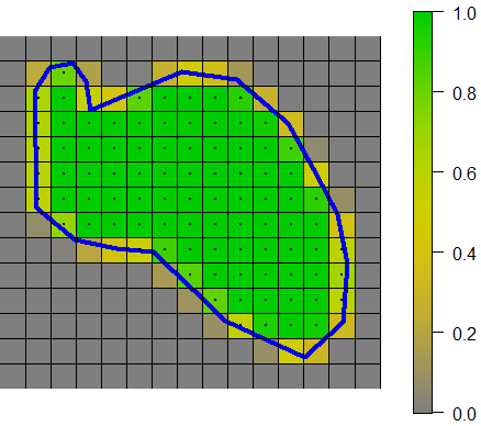
  where $\Delta=\Pi_{i=1}^{d}\Delta_{i}$, and $\mathcal{I}_{B_{i}}$ is a weighted version of the indicator function $I_{B_{i}}$. Each grid point can be associated with a surrounding grid box, and $\mathcal{I}_{B}$ at a grid point is equal to the fraction of the area of the associated grid box that is contained in $B$. Values for $\mathcal{I}_{B}$ will be mostly zero or one with fraction values for grid boxes on the boundary of $B$. In two dimensions one can evaluate an approximate version of $\mathcal{I}_{B}$ rapidly, and an example is illustrated in Figure 1.

Our method approximates the integrals shown in Eqn. (9) with discretized sums over a finite domain as shown in Eqn. (10), exploiting the fast Fourier transform (FFT) algorithm to compute the DFT. The algorithm to determine an entry of $K$ is as follows. Throughout this algorithm we will use $\theta_{x}$ to refer to the distance where the correlation function decreases to $x$.

1. 1.

   A regular grid $G$ is constructed which extends beyond the regions ${B_{1},...,B_{n}}$. The overall extent of the grid is constrained to be at least twice $\theta_{0.05}$ and also extend beyond all observation regions by at least $\theta_{0.25}$. The grid size is chosen to be highly composite (dyadic) to facilitate an efficient FFT.

2. 2.

   $\widehat{\mbox{\boldmath$B$}}^{i}=DFT[\mathcal{I}_{B_{i}}]$ is found by FFT for $i=1,\dots,n$.

3. 3.

   $\widehat{\mbox{\boldmath$c$}}=DFT[c]$ is found for $c(\cdot)$ by FFT.

4. 4.

   $\widehat{|B_{i}|}=\sum\mathcal{I}_{B_{i}}(G)\Delta$ is found for $i=1,\dots,n$.

5. 5.

   $\mbox{\boldmath$K$}_{i,j}=\frac{1}{\widehat{|B_{i}|}}\frac{1}{\widehat{|B_{j}|}}\sum_{k}\widehat{\mbox{\boldmath$B$}}^{i}_{k}\overline{\widehat{\mbox{\boldmath$B$}}^{j}_{k}}\widehat{\mbox{\boldmath$c$}}_{k}\Delta$ are found with the sum being over the discretized Fourier frequencies prescribed by the DFT.

The grid extent constraints are motivated by two factors. The discrete, finite domain approximation to the full Fourier transform of $c$ degrades significantly when the grid is constructed over a domain which is small relative to the decay rate of the covariance function. This is due to the well known property of the DFT as enforcing a periodic representation of the covariance function. Extending the grid to be at least twice $\theta_{0.05}$ avoids this issue. Also, the discrete, finite domain approximation degrades significantly without a ‘buffer zone’ around the regions ${B_{1},...,B_{n}}$ based on correlation range. This is due to the periodic wrapping of the approximation to the covariance whereby regions on one edge of the domain become (spuriously) correlated with regions on the opposite edge. Experiments show that extending the grid with a buffer of $\theta_{0.25}$ avoids this artifact. Thus, if the spatial domain that contains the regions ${B_{1},...,B_{n}}$ is a square with a length $L$, a conservative grid for computation should be extended to have extent of at least $max(L+2\theta_{0.25},2\theta_{0.05})$. The larger the extent of the grid, the more these effects are minimized, but larger extents at a fixed grid resolution also result in coarser evaluations of the functions in question.

The accuracy of this method is also a function of the resolution of the grid. In Section 3.1 we provide a numerical study to suggest the relationship between grid spacing ($\Delta$), extent, and accuracy.

The proposed FAIR algorithm also provides intermediate quantities to make surface prediction (see, Eqn. (4)) efficient. In particular, the fine grid $G$ (containing $L$ points), used for the computation of the change of support integrals, can be reused for creating a predicted surface. To simplify the exposition we will assume throughout this section that $\mbox{\boldmath$\mu$},\mu_{Y}^{\cdot},\tau^{2}$ and any additional parameters in $c_{Y}$ are known. Now, motivated by Eqn. (4 ) one can define the vector

Now focusing on the second term of Eqn. (5) and an arbitrary $i$-th member of the grid, denoted by $\mbox{\boldmath$u$}_{i}$, we have:

where $\phi(\mbox{\boldmath$u$})=\sum_{\ell=1}^{n}\frac{\mbox{\boldmath$\beta$}_{\ell}}{|B_{\ell}|}I_{B_{\ell}}(\mbox{\boldmath$u$})$. Note that the last expression is a convolution of $\phi$ with $c$ evaluated at $\mbox{\boldmath$u$}_{i}$; using the same discrete approximation described above we are lead to

where $DFT(\phi)$ and $DFT(c)$ have support on the mirror grid in the frequency domain, and $\mu_{Y}(G)=\{\mu_{Y}(\mbox{\boldmath$u$}_{i})\}_{i=1}^{L}$. Note that the $i^{th}$ component of $\widehat{\mbox{\boldmath$Y$}}^{G}$ is the predicted value at $\mbox{\boldmath$u$}_{i}$. Thus, evaluation of the predicted surface on the entire grid $G$ is $\widehat{\mbox{\boldmath$Y$}}^{G}$, obtained in a single step using the inverse DFT. Additionally, note that $DFT[\phi]=\sum_{\ell=1}^{n}\frac{\mbox{\boldmath$\beta$}_{\ell}}{|B_{\ell}|}DFT[I_{B_{\ell}}]\approx\sum_{\ell=1}^{n}\frac{\mbox{\boldmath$\beta$}_{\ell}}{\widehat{|B_{\ell}|}}DFT[\mathcal{I}_{B_{\ell}}]$, and from evaluation of $\beta$, $\widehat{|B_{\ell}|}$ as well as $DFT[\mathcal{I}_{B_{\ell}}]$ for each $B_{\ell}$ and $DFT[c]$ have already been computed.

In this section, we consider the underlying process $Y(\mbox{\boldmath$s$})$ being averaged over two rectangular regions with sides parallel to the coordinate axes. In particular, the regions are $A=[ax_{1},ax_{2}]\times[ay_{1},ay_{2}]$ and $B=[bx_{1},bx_{2}]\times[by_{1},by_{2}]$, respectively. Then straightforward calculation yields,

where $\Phi(.)$ denotes the cumulative distribution function of a Normal(0,1) random variable. Note that the integrals in Eqn. (11) are of the same general type and can be computed using integration by parts.

For our accuracy studies, we consider pairs of unit squares $A=[0,1]^{2}$ and $B_{i}=[\delta_{i},1+\delta_{i}]^{2}$, where the offset $\delta_{i}$ is a separation distance between the regions. For each $\delta_{i}$, the ground truth covariance matrix for the two averaged regional values was computed. The ground truth correlation between regions varies with their separation distance - some representative values are shown in Table 1.

For each, we employ FAIR to approximate the covariance matrix using varying grids (in each case, using the default image radius and region padding selection method as described in Section 2.2. The grid resolution was varied over integer powers of two: the coarsest grid consisted of $2^{3}\times 2^{3}=8\times 8=64$ total grid points, while the finest grid had $2^{11}\times 2^{11}=2048\times 2048\approx$ 4 million points. The approximated covariance matrices are used to generate correlations, which are then compared against the ground truth values. The absolute errors observed during these studies are shown in Figure 2.

Overall, our method does an excellent job in terms of accuracy and as one would expect, accuracy improves with increased grid resolution, until hitting a plateau. Note that shape pairs with smaller offsets reach this plateau at lower resolutions than pairs with larger offsets. This plateau represents the transition from accuracy being constrained by grid resolution to being constrained by grid extent. When the study is repeated with larger grid extents (in this instance, increasing default extent constraints by a single unit, i.e., extent set to $max(L+2\theta_{0.25}+1,2\theta_{0.05}+1)$), the plateau appears at lower error values/higher grid resolutions, as shown in Figure 3, but there is also a decrease in accuracy at lower resolutions for most of the offset distances. This loss of accuracy is due to coarser grids (spreading the same number of grid points over a larger extent), which then lead to coarser evaluations of the functions involved.

In this section, we demonstrate the performance of the algorithm with a spatial dataset, specifically a spatial estimation and prediction problem using real-world data and region geometry.

The region geometry selected for this study are the 84 US Census blocks entirely contained in the region that extends from 104.85 to 104.75 West Longitude, and from 38.8 to 38.9 North Latitude (a region covering some of Colorado Springs, CO) as indicated in Figure 5. The data chosen are the block-level counts of traffic intersections (an indicator of economic development). Intersection data made available by Patricia Romero Lankao from the National Energy Renewable Laboratory and aligned with the 2016 census block group shape files, obtained from https://www2.census.gov/geo/tiger/ as GENZ2016 2016 Cartographic Boundary Files (cb_2016_08_bg_500k)¹¹ 1 This data set is compiled by The Center for Neighborhood Technology (cnt.org) and distributed in support of the Housing and Transportation (H+T) Affordability Index. State by state files in cvs format are available for download from https://htaindex.cnt.org/.

We shift and rescale the region geometry to occupy a unit square at $[0,1]^{2}$, transform the count data to densities by dividing by block area, and then normalize the density data using the observed sample mean and standard deviation. The transformed data are shown in Figure 6.

We model the normalized data as block averages of an underlying Gaussian process with a Matérn covariance. We assume a smoothness of 1.5, and estimate the marginal variance, range, and (post-aggregation) nugget variance using maximum likelihood methods - to facilitate the timing comparison, we concentrate the marginal variance and nugget variance into a ratio term, and perform a simple grid search over (range parameter, variance ratio) candidate pairs - 9 distinct range candidates were considered between 0.0625 and 0.50, with 45 distinct variance ratio candidates between 0.005 and 2.0. FAIR was implemented with a $2^{10}\times 2^{10}$ grid extending approximately to $[-2,3]^{2}$. Riemann quadrature points were subsampled from the FAIR grid, ranging from163 points in the smallest region, up to 2593 points in the largest region, with a mean of 414 points per region.

Each range parameter candidate investigated requires the recalculation of the regional covariance matrix. For each candidate, these calculations were repeated using both the FAIR algorithm and the standard Riemann one. Because the region geometry does not vary across these calculations, some quantities can be precomputed (the Fourier transforms of the fractional indicator functions in the case of FAIR, and the coordinates of the quadrature points in each region in the case of Riemann). For larger range parameter candidates, some matrices returned by FAIR were not quite positive definite, and were thus coerced to the nearest positive definite matrix using Matrix::nearPD in R. Additionally, the geometry of these regions (while still polygonal) is more complex than in our previous studies, with a mean side count of 12. These factors contribute to differing cost ratios in this study, relative to those observed in the study described in Section 3.2. Timing results for the major phases of each algorithm for this estimation task are provided in Tables 6 and 7.

With covariance parameter estimates found, we use the values computed by the FAIR algorithm during the estimation process to predict the underlying surface on the default grid. As noted in Section 2.3, this involves only a weighted sum of the Fourier-transformed indicator functions to form $DFT[\phi]$, an entry-wise product of the $DFT[\phi]$ and $DFT[c]$ terms, and an inverse FFT, and incurs only 2.02s of additional compute time. A subset of the predicted surface is shown in Figure 6 (only a subset is provided, as away from the observation regions, the prediction reverts to the mean).

We note that this model does not provide high predictive power in this case, with both algorithms finding parameter MLEs at the boundary of the search grid. We reiterate that the goal of this study is not to produce a high-quality model for this particular dataset, rather to employ the competing algorithms in a typical spatial estimation task for a realistic comparison of relative performance, and to demonstrate the low cost of surface prediction having performed an estimation task with FAIR.

References

- [1] Jonathan Bradley, Scott Holan, and Christopher Wikle. Multivariate spatio-temporal models for high-dimensional areal data with application to Longitudinal Employer-Household Dynamics. Annals of Applied Statistics, 9:1761–1791, 2015.
- [2] Jonathan Bradley, Christopher Wikle, and Scott Holan. Spatio-temporal change of support with application to American Community Survey multi-year period estimates. Stat, 4:255–270, 2015.
- [3] Jonathan Bradley, Christopher Wikle, and Scott Holan. Regionalization of multi-scale spatial processes by using a criterion for spatial aggregation error. Journal of the Royal Statistical Society: Series B (Statistical Methodology), 79:815–832, 2016.
- [4] Noel Cressie. Statistics for Spatial Data. Wiley, revised edition, 1993.
- [5] Carol A. Gotway and Linda J. Young. Combining incompatible spatial data. Journal of the American Statistical Association, 97(458):632–648, 2002.
- [6] A. G. Journel and Ch. J. Huijbregts. Mining Geostatistics. Blackburn Press, 2004.
- [7] R. J. Martin and J. N. Dwyer. Approximations to the covariance properties of processes averaged over irregular spatial regions. Communications in Statistics, Theory and Methods, 23(3):913–945, 1994.
- [8] Hai Nguyen, Noel Cressie, and Amy Braverman. Spatial statistical data fusion for remote sensing applications. Journal of the American Statistical Association, 107(499):1004–1018, 2012.
- [9] Hai Nguyen, Matthias Katzfuss, Noel Cressie, and Amy Braverman. Spatio-temporal data fusion for very large remote sensing datasets. Technometrics, 56(2):174–185, 2014.
- [10] Douglas Nychka, Soutir Bandyopadhyay, Dorit Hammerling, Finn Lindgren, and Stephan Sain. A multiresolution Gaussian process model for the analysis of large spatial datasets. Journal of Computational and Graphical Statistics, 24(2):579–599, 2015.
- [11] Hae Ryoung Song, Montserrat Fuentes, and Sujit Ghosh. A comparative study of Gaussian geostatistical models and Gaussian Markov random field models. Journal of Multivariate Analysis, 99(8):1681–1697, 2008.