A Precise Analytical Approximation for the Deprojection of the Sérsic ProfilePreprint: Eduardo Vitral,
Abstract
The Sérsic model is known to fit well the surface brightness (or surface density) profiles of elliptical galaxies and galaxy bulges, and possibly for dwarf spheroidal galaxies and globular clusters. The deprojected density and mass profiles are important for many astrophysical applications, in particular for mass-orbit modeling of these systems. However, the exact deprojection formula for the Sérsic model employs special functions not available in most computer languages. We show that all previous analytical approximations to the 3D density profile are imprecise at low Sérsic index (). We have derived a more precise analytical approximation to the deprojected Sérsic density profile by fitting two-dimensional 10th-order polynomials to the differences of the logarithms of the numerical deprojection and of the analytical approximation by Lima Neto et al. 1999 (Lima Neto et al. 1999, LGM) of the density profile on one hand and of the mass profile on the other. Our LGM-based polynomial fits have typical relative precision better than 0.2% for both density and mass profiles, for Sérsic indices and radii . Our approximation is much more precise than those of LGM, Simonneau & Prada 1999; Simonneau & Prada 2004, Trujillo et al. 2002 for non-half-integer values of the index, and of Emsellem & van de Ven 2008 for non-one-tenth-integer values with , and are nevertheless more than 0.2% precise for larger Sérsic indices, for both density and mass profiles. An appendix compares the deprojected Sérsic profiles with those of the popular simple models from Plummer 1911, Jaffe 1983, Hernquist 1990, Navarro et al. 1996, and Einasto 1965.
Key Words.
Galaxies: structure – Galaxies: bulges – Galaxies: elliptical and lenticular, cD – (Galaxy:) globular clusters: general – Methods: numerical1 Introduction
The Sérsic model (Sérsic 1963; Sersic 1968) is the generalization of the law (de Vaucouleurs 1948) to describe the surface brightness profiles of elliptical galaxies (Caon et al. 1993) and the bulges of spiral galaxies (Simard et al. 2011). It has also been used to describe the surface density profiles of nuclear star clusters (Carson et al. 2015), resolved dwarf spheroidal galaxies (Battaglia et al. 2006) and globular clusters (Barmby et al. 2007).
The surface (mass or number) density (or equivalently surface brightness) of the Sérsic model is
| (1) |
where is the projected distance to the source center in the plane-of-sky (POS), is the effective radius containing half of the projected luminosity, is the Sérsic index and is the central surface density. The term is a function of , obtained by solving the equation:
| (2) |
where is the lower incomplete gamma function.
Since the Sérsic model represents well astronomical objects viewed in projection, it is important to know its corresponding three-dimensional (3D) density and mass profiles. These serve as a reference to compare to other possible observational tracers, as well as to dark matter. Moreover, the 3D density profile is required for modeling the kinematics of spherical structures, since it appears in the Jeans equation of local dynamical equilibrium. Since the Jeans equation also contains the total mass profile, the 3D mass profiles of stellar components are required to estimate the dark matter mass profile of elliptical and dwarf spheroidal galaxies.
Many authors assume that simple three-dimensional models resemble Sérsic models for certain values of the Sérsic index: It is often assumed that massive ellipticals and spiral bulges are well represented by the Hernquist 1990 model (e.g., Widrow & Dubinski 2005). On the other hand, dwarf spheroidal galaxies are often described as a Plummer 1911 model (e.g. Muñoz et al. 2018, who also tried Sérsic and other models), while ultra diffuse galaxies have been described by Einasto (Einasto 1965; Navarro et al. 2004) models (Nusser 2019). Łokas & Mamon 2001 noted that the projected Navarro et al. 1996 (Navarro et al. 1996, hereafter NFW) model resembles an Sérsic for reasonable concentrations. Finally, Sérsic models are considered to resemble the Jaffe 1983 model (Ciotti et al. 2019). In Appendix A, we compare these models to the deprojected Sérsic.
Unfortunately, the deprojection of the Sérsic surface density profile to a 3D (mass or number)11 1 The number profile always has the same form as the mass profile, and is obtained by simply replacing by and by , e.g. in Eqs. (6), (7), and (17). density profile, through Abel 1826 inversion
| (3) |
(e.g., Binney & Mamon 1982), as well as the corresponding 3D mass (or number) profile
| (4) |
both involve the complicated Meijer G special function (Mazure & Capelato 2002 for integer values of , and Baes & Gentile 2011 for general values of ) or the other complicated Fox function (Baes & van Hese 2011), neither of which are available in popular computer languages.
Following the shape of the analytical approximation to the law by Mellier & Mathez 1987, Prugniel & Simien 1997 (Prugniel & Simien 1997, hereafter, PS) proposed an analytical approximation for the 3D density of the Sérsic profile:
| (5) |
which yields a simple analytical form for the 3D mass profile
| (6) | |||||
| (7) |
where is a function depending only on . PS calculated this dependence to be:
| (8) |
while Lima Neto et al. 1999 (hereafter, LGM) later perfected this approximation with
| (9) |
LGM indicate that equation (9) is good to 5 per cent relative accuracy for and . However, the power-law approximation at small radii is unjustified for small . Indeed, as shown by Baes & Gentile 2011, the central density profile converges to a finite value for (and the inner density profile diverges only logarithmically for ), as we will illustrate in Sect. 3.
Simonneau & Prada 1999 (Simonneau & Prada 1999, Simonneau & Prada 2004, hereafter SP) proposed the quasi-Gaussian expansion for the density profile
| (10) |
where
| (11) | |||||
| (12) |
where and are 10 fit parameters. The individual SP density profiles (the terms inside the sum of Eq. 10) have a similar (but not the same) form as the PS/LGM one, hence a similar shape for the mass profile:
| (13) | |||||
Trujillo et al. 2002 proposed an ellipsoid formula, which in the limit of spherical symmetry becomes
| (14) |
where is the modified Bessel function of the 2nd kind22 2 Trujillo et al. 2002 call this the modified Bessel function of the 3rd kind, as some others do. of index , while , , , , and are empirical functions of index . Trujillo et al. 2002 only provided their results for integer and half-integer values of for and only integer values of beyond.
Emsellem & van de Ven 2008 (Emsellem & van de Ven 2008, hereafter EV) repeated their analysis on a finer grid of , with steps of 0.1 for and with one more term, , in equation (14), involving 168 parameters. Unfortunately, as shown in Figure 1, these functions vary abruptly for . Moreover, neither Trujillo et al. 2002 nor Emsellem & van de Ven 2008 provide analytical forms for the mass profile.
In summary, all the previous approximations to the deprojected Sérsic model have drawbacks:
- •
PS, LGM (and Márquez et al. 2000, which is the same as LGM, but with a slightly different last term for , which was a typo) are inappropriate for low (Baes & Gentile 2011) and less precise than claimed (Emsellem & van de Ven 2008).
- •
SP is limited to , and is generally less precise than EV.
- •
Trujillo et al. 2002 is only given for half-integer values of and their parameters vary wildly with for . They do not provide a formula for the mass profile.
- •
EV also suffers from discrete values of , even though the grid is finer ( for ). EV also did not provide a formula for the mass profile.
In this article, we provide polynomial fits to the log residuals of the LGM approximation, allowing to reach high accuracy for both the 3D density and 3D mass profiles in a wide range of Sérsic indices. In Sect. 2, we present the mathematical formalism and briefly explain our numerical integration method. We then show in Sect. 3 how our polynomial plus LGM approximation is orders of magnitude more precise than the formulae of LGM, SP, and Trujillo et al. 2002, as well as that of EV for low and only slightly worse for . We conclude and discuss our results in Sect. 4.
2 Method
2.1 Equations using dimensionless profiles
We express the general surface density, 3D density, and 3D mass (or number) profiles in terms of dimensionless functions:
| (15) | |||||
| (16) | |||||
| (17) |
Hereafter, we will use and . For the Sérsic model, the dimensionless surface density profile is
| (18) |
while for the PS model, one can write the dimensionless 3D density and mass profiles as
| (19) | |||||
| (20) |
2.2 Numerical integration
We numerically evaluated the dimensionless 3D density (Eq. [21]) and mass (Eq. [24]) profiles by peforming the numerical integrations in cells 50 100 of , with and . Numerical calculations were done with Python’s scipy.integrate.quad. For both density and mass profiles, we split the numerical integration in two, i.e.
| (25) |
where and . We used a relative tolerance of and in both integrals. If , we also used and , but for a single integral from to .
We performed our analysis using either the highly accurate approximations for of Ciotti & Bertin 1999 (Ciotti & Bertin 1999, hereafter, CB) or the exact (numerical) solutions of Eq. (2). We noticed that the difference between these two approaches was negligible (see Sect. 3).
We then fit two-dimensional polynomials to both and , for geometrically spaced and , i.e. writing
| (26) |
with polynomial orders . For this, we used Python’s package numpy.linalg.lstsq. We found the smallest residuals for order 10 polynomials when using both the approximation of CB and by numerically solving Eq. (2). The coefficients are provided in Tables 2, 3, 4 and 5 in Appendix B. In the rest of the paper, we present the results relative to the CB approximation, since it is a simpler and more used model, and also because our order 10 polynomial fits remarkably well the exact case.
2.3 Numerical precision: Tests for known simple analytical deprojections ( and )
For Sérsic indices and , there are analytical solutions for the 3D density profile:
| (27) |
where is the modified Bessel function of the second kind of index 0. We can therefore verify the numerical integration of Eq. (21) for these two Sérsic indices.
For the interval , we compared the densities from numerical integration with the analytical formulae of Eq. (27), using the CB approximation for . The match is very good, with root-mean-square (rms) values of of and for and , respectively. The same comparison using the exact yields and , respectively (with one particular value of causing the higher rms for ).
3 Results
As seen in Figure 2, the 3D density profiles depart from the power laws proposed by LGM at low , especially for low radii, as expected by the asymptotic expansions of Baes & Gentile 2011 for . Interestingly, the LGM formula is also inadequate at low radii for and 2.25, although the asymptotic expansion of Baes & Gentile 2011 indicate power-law behavior at small radii. This poor accuracy of the LGM approximation at low radii is a serious concern when performing kinematic modeling of systems with possible central massive black holes. For example, Gaia DR2 positions and proper motions for stars in nearby globular clusters extend inwards to 0.7 arcsec from the center, which translates to .
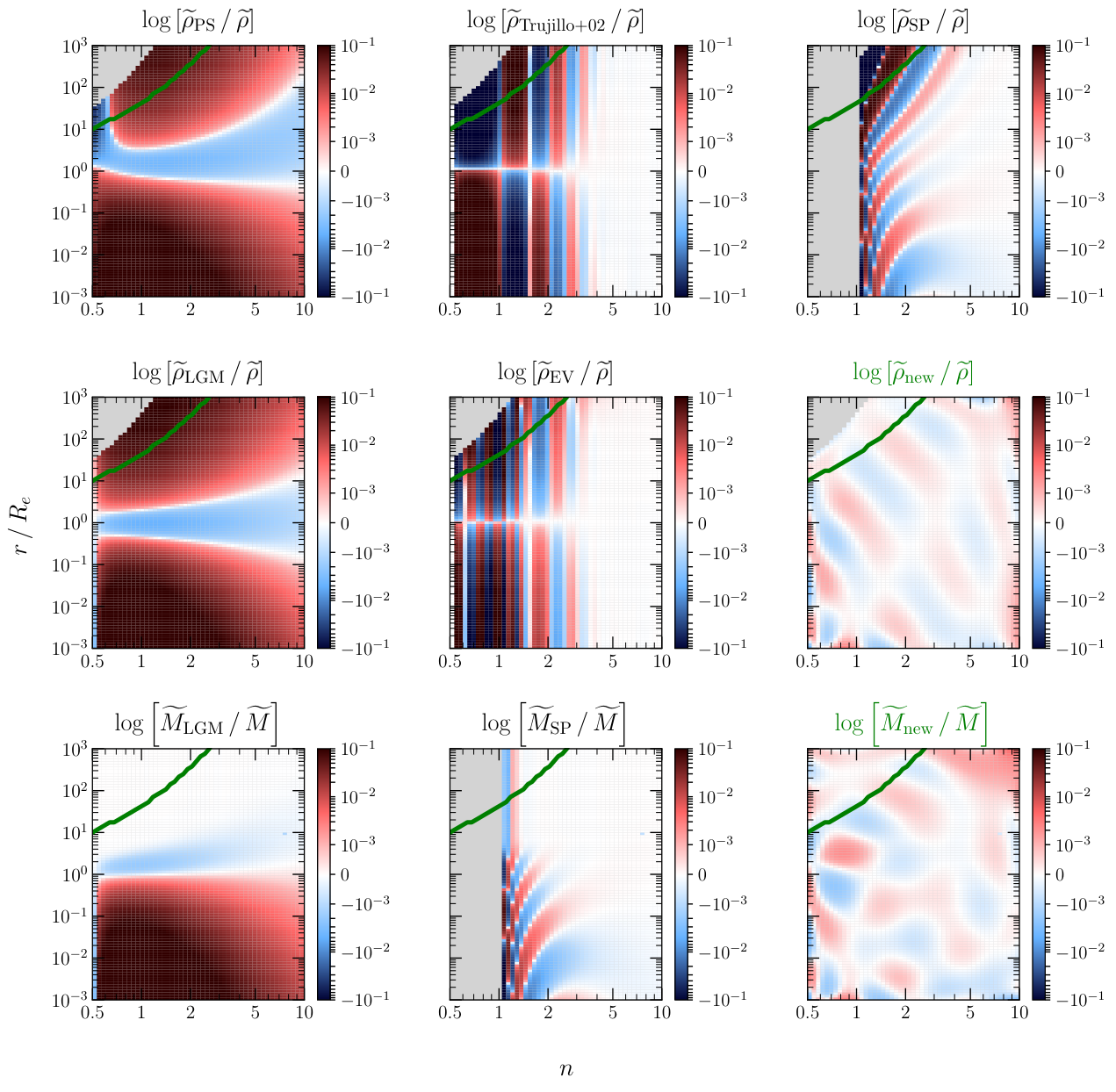
We now compare the accuracy of the different analytical approximations for the 3D density and 3D mass profiles. Figure 3 displays the ratio , for and , for the main analytical approximations available in the literature, along with our new model
| (28) |
where is either the 3D density or 3D mass profile. We see that our model presents a more continuous behavior over the full range of Sérsic indices and radii. Our approximation displays the smallest residuals among all models for (except that SP outperforms our model for mass estimates at for ).
The variation of accuracy with Sérsic index can be seen in more detail in Figure 4, which displays the rms of , over the radial domain where , of the main analytical approximations, using 1000 log-spaced Sérsic indices. Figure 4 indicates that the SP (respectively, EV) approximation for density has rms relative accuracy worse than 2.3% (0.01 for ) for (respectively 1.3). Our approximation (Eq. [28]) is more accurate than SP for (density) and (mass), and is more accurate than EV for (density), except for their particular choices of . Figure 4 shows that the EV approximation is much more accurate at specific values of (note that our grid does not contain all of these values precisely, so the EV approximation is even more accurate at these specific values of ). However, these specific values of represent a negligible measure compared to the full continuous range of . Therefore, the EV approximation at low is not reliable for estimating the 3D density profile.
We analyzed the results shown in Figure 4 using from either CB or by numerically solving Eq. (2), and the results were very similar. In fact, the results are similar if we adopt one form of in the numerical integration and the other in the analytical approximations. This can be explained by the fact that is practically the same for both estimates of , yielding a very similar fit of Eq. (26).
Finally, we provide in Table 1 the rms accuracies computed over the full range of radii and , except for the SP formula, which does not allow , and also avoiding the domain where . We see that, averaging over all Sérsic indices, our approximation is much more accurate than all others (with over 10 times lower rms).
| rms | rms | |
| Author | ||
| Prugniel & Simien 97 | 0.1052 | 0.1187 |
| Lima Neto et al. 99 | 0.0905 | 0.1021 |
| Simonneau & Prada 04 () | 0.0238 | 0.0098 |
| Trujillo et al. 02 | 0.1496 | – |
| Emsellem & van de Ven 08 | 0.0382 | – |
| new | 0.0005 | 0.0007 |
| hybrid-1 (optimized for ) | 0.0004 | 0.0005 |
| hybrid-2 (optimized for ) | 0.0004 | 0.0005 |
Notes: The rms accuracies are computed over the full range of radii (100 steps) and (50 steps), except for the SP formula, which does not allow , and also avoiding the domain where . Trujillo et al. 2002 and EV do not provide analytical mass profiles. The lower two rows display hybrid models, both with our new approximation for and for . The first hybrid model has a mass profile for and for , while in hybrid model 2, the mass profile is for and for .
4 Conclusions and Discussion
The Sérsic model is usually considered to provide excellent fits to the surface density (or surface brightness) profiles of elliptical galaxies, spiral bulges, and even dwarf spheroidal galaxies and globular clusters. In the past, many authors have used simple analytical models to describe these systems, arguing that their models, once projected, resemble Sérsic models. It is more relevant to compare the physically meaningful three-dimensional density profiles of these simple models to the deprojected Sérsic model.
This comparison is made in Appendix A for the Plummer, Jaffe, Hernquist, Einasto, and NFW models. As seen in Fig. 5, most of the simple models do not provide decent fits to the deprojected Sérsic model, even for narrow ranges of the Sérsic index. The Plummer model requires a low index at small radii, but a much higher index at large radii, and the normalized density profile fits poorly at most radii. The Hernquist model resembles the deprojected Sérsic model at low radii and the Sérsic at large radii. The NFW models resemble the deprojected Sérsic at low radii (consistent with the similarity of the projected Sérsic with NFW discovered by Łokas & Mamon 2001), but have a shallower slope at large radii than even the shallowest () deprojected Sérsic model. On the other hand, the Jaffe model resembles the model at all radii. Moreover, as seen in Figure 6, the Einasto model provides a fair representation (rms difference of density profiles normalized to value at half-mass radius less than 0.1 dex) of the deprojected Sérsic model for .
We reconsidered the different analytical deprojections of the Sérsic surface brightness (or surface density) profile. We found that the analytical approximations present in the literature do not show satisfying results when the Sérsic index is in the range (apart from the specific values of given by Emsellem & van de Ven 2008). In particular, the power-law times exponential density profile of Prugniel & Simien 1997 and Lima Neto et al. 1999 fails to reproduce the inner density profiles for low , even up to despite the power-law behavior expected at small radii for (Baes & Gentile 2011).
With an order 10 two-dimensional polynomial fit, we propose a new analytical approximation (Eq. [28]) that is precise over the range , for . Our approximation provides the highest precision when averaging over all values of Sérsic indices and radii (Table 1). While the approximations of Simonneau & Prada 1999; Simonneau & Prada 2004 on one hand and of Emsellem & van de Ven 2008 on the other, are more accurate than ours for and 3.4, respectively, ours is more accurate at lower Sérsic indices.
This is important for the study of astronomical sources with low Sérsic indexes, such as galaxy bulges, nuclear star clusters, dwarf spheroidal galaxies, and globular clusters. Moreover, our approximation of Eq. (28) to the density profile is sufficiently accurate for most scientific analyses for . But the user could use a hybrid approximation, combining either the Simonneau & Prada 2004 or Emsellem & van de Ven 2008 approximations for and ours for (as shown in the last rows of Table 1). Finally, our analysis has the advantage of also providing a precise approximation for the mass profile, whereas no analytical expression can be derived from the density profile of Emsellem & van de Ven 2008. Our Python 3 codes are available at https://github.com/eduardo-vitral/Vitral_Mamon2020a along with coefficients of Tables 2 and 3.
These results will be useful in future mass-orbit modeling analyses of low-mass spherical systems, as we are preparing for globular clusters (Vitral & Mamon, in prep.).
References
- Abel (1826) Abel, N. H. 1826, Journal für die reine und angewandte Mathematik, 1, 153
- Baes & Gentile (2011) Baes, M. & Gentile, G. 2011, A&A, 525, A136
- Baes & van Hese (2011) Baes, M. & van Hese, E. 2011, A&A, 534, A69
- Barmby et al. (2007) Barmby, P., McLaughlin, D. E., Harris, W. E., Harris, G. L. H., & Forbes, D. A. 2007, AJ, 133, 2764
- Battaglia et al. (2006) Battaglia, G., Tolstoy, E., Helmi, A., et al. 2006, A&A, 459, 423
- Binney & Mamon (1982) Binney, J. & Mamon, G. A. 1982, MNRAS, 200, 361
- Caon et al. (1993) Caon, N., Capaccioli, M., & D’Onofrio, M. 1993, MNRAS, 265, 1013
- Carson et al. (2015) Carson, D. J., Barth, A. J., Seth, A. C., et al. 2015, AJ, 149, 170
- Ciotti & Bertin (1999) Ciotti, L. & Bertin, G. 1999, A&A, 352, 447
- Ciotti et al. (2019) Ciotti, L., Mancino, A., & Pellegrini, S. 2019, MNRAS, 490, 2656
- de Vaucouleurs (1948) de Vaucouleurs, G. 1948, Annales d’Astrophysique, 11, 247
- Einasto (1965) Einasto, J. 1965, Trudy Inst. Astroz. Alma-Ata, 51, 87
- Emsellem & van de Ven (2008) Emsellem, E. & van de Ven, G. 2008, ApJ, 674, 653
- Hernquist (1990) Hernquist, L. 1990, ApJ, 356, 359
- Jaffe (1983) Jaffe, W. 1983, MNRAS, 202, 995
- Lima Neto et al. (1999) Lima Neto, G. B., Gerbal, D., & Márquez, I. 1999, MNRAS, 309, 481
- Łokas & Mamon (2001) Łokas, E. L. & Mamon, G. A. 2001, MNRAS, 321, 155
- Márquez et al. (2000) Márquez, I., Lima Neto, G. B., Capelato, H., Durret, F., & Gerbal, D. 2000, A&A, 353, 873
- Mazure & Capelato (2002) Mazure, A. & Capelato, H. V. 2002, A&A, 383, 384
- Mellier & Mathez (1987) Mellier, Y. & Mathez, G. 1987, A&A, 175, 1
- Muñoz et al. (2018) Muñoz, R. R., Côté, P., Santana, F. A., et al. 2018, ApJ, 860, 66
- Navarro et al. (1996) Navarro, J. F., Frenk, C. S., & White, S. D. M. 1996, ApJ, 462, 563
- Navarro et al. (2004) Navarro, J. F., Hayashi, E., Power, C., et al. 2004, MNRAS, 349, 1039
- Nusser (2019) Nusser, A. 2019, arXiv e-prints, arXiv:1907.08035
- Plummer (1911) Plummer, H. C. 1911, MNRAS, 71, 460
- Prugniel & Simien (1997) Prugniel, P. & Simien, F. 1997, A&A, 321, 111
- Sérsic (1963) Sérsic, J. L. 1963, Bull. Assoc. Argentina de Astron., 6, 41
- Sersic (1968) Sersic, J. L. 1968, Atlas de galaxias australes (Cordoba, Argentina: Observatorio Astronomico)
- Simard et al. (2011) Simard, L., Mendel, J. T., Patton, D. R., Ellison, S. L., & McConnachie, A. W. 2011, ApJS, 196, 11
- Simonneau & Prada (1999) Simonneau, E. & Prada, F. 1999, unpublished preprint, submitted to MNRAS, arXiv:astro-ph/9906151
- Simonneau & Prada (2004) Simonneau, E. & Prada, F. 2004, Rev. Mexicana Astron. Astrofis., 40, 69
- Trujillo et al. (2002) Trujillo, I., Asensio Ramos, A., Rubiño-Martín, J. A., et al. 2002, MNRAS, 333, 510
- Widrow & Dubinski (2005) Widrow, L. M. & Dubinski, J. 2005, ApJ, 631, 838
Appendix A Comparison of deprojected Sérsic to other popular models
Figure 5 compares the density profiles, normalized to the half-mass radius , for which we applied the following relations:
| (29) |
The ratio of half-mass radius to scale radius is given by
| (30) |
In Eq. (30) for NFW, , where is the maximum allowed radius (because, contrary to all other models discussed here, the NFW model has logarithmically divergent mass). Also, for Einasto, is the inverse regularized lower incomplete gamma function, i.e. satisfies .33 3 The inverse (regularized) incomplete gamma function is available in many computer languages, e.g. Python (scipy package), Fortran, Matlab, Mathematica, and Javascript. For Sérsic, the conversion was done by fitting a order 3 polynomial and recovering the relation , where .
The Einasto model, which is the 3D analog of the Sérsic model, resembles the deprojected Sérsic model. Figure 6 shows the best-fit values of the Einasto index, in terms of the Sérsic index. The relation (red curve) is almost one-to-one (dashed line). The figure also shows the rms over all radii and best-fit indices (blue curve).
Appendix B Coefficients of polynomials for new deprojected Sérsic models
In this section, we present Tables 2, 3, 4 and 5, containing the coefficients in Eq. (26), for and , as well as for both Ciotti & Bertin 1999 approximation for and the exact solution from Eq. (2). The numbers in parentheses are the exponents: e.g. “” corresponds to . Coefficients that are not followed by a number in parentheses have exponent zero.
| \ | 0 | 1 | 2 | 3 | 4 | 5 | 6 | 7 | 8 | 9 | 10 |
|---|---|---|---|---|---|---|---|---|---|---|---|
| 0 | |||||||||||
| 1 | – | ||||||||||
| 2 | – | – | |||||||||
| 3 | – | – | – | ||||||||
| 4 | – | – | – | – | |||||||
| 5 | – | – | – | – | – | ||||||
| 6 | – | – | – | – | – | – | |||||
| 7 | – | – | – | – | – | – | – | ||||
| 8 | – | – | – | – | – | – | – | – | |||
| 9 | – | – | – | – | – | – | – | – | – | ||
| 10 | – | – | – | – | – | – | – | – | – | – |
| \ | 0 | 1 | 2 | 3 | 4 | 5 | 6 | 7 | 8 | 9 | 10 |
|---|---|---|---|---|---|---|---|---|---|---|---|
| 0 | |||||||||||
| 1 | – | ||||||||||
| 2 | – | – | |||||||||
| 3 | – | – | – | ||||||||
| 4 | – | – | – | – | |||||||
| 5 | – | – | – | – | – | ||||||
| 6 | – | – | – | – | – | – | |||||
| 7 | – | – | – | – | – | – | – | ||||
| 8 | – | – | – | – | – | – | – | – | |||
| 9 | – | – | – | – | – | – | – | – | – | ||
| 10 | – | – | – | – | – | – | – | – | – | – |