跳到论文正文
W Papers独立论文阅读器 arXiv:2001.02853 论文正文 计算阅读时间 · 0%
引用这篇论文根据当前论文元数据生成,正式投稿前建议核对。


License: arXiv.org perpetual non-exclusive license
arXiv:2001.02853v2 [hep-ph] 04 May 2020

Vector-like Quark Interpretation for the CKM Unitarity Violation, Excess in Higgs Signal Strength, and Bottom Quark Forward-Backward Asymmetry

Kingman Cheung1,2,3,4, Wai-Yee Keung5, Chih-Ting Lu6, and Po-Yan Tseng7 Affiliation: 1 Physics Division, National Center for Theoretical Sciences, Hsinchu, Taiwan
2 Department of Physics, National Tsing Hua University, Hsinchu 300, Taiwan
3 Division of Quantum Phases and Devices, School of Physics, Konkuk University, Seoul 143-701, Republic of Korea
4 Department of Physics, National Central University, Chungli, Taiwan
5 Department of Physics, University of Illinois at Chicago, Illinois 60607 USA
6 School of Physics, KIAS, Seoul 130-722, Republic of Korea
7Department of Physics and IPAP, Yonsei University, Seoul 03722, Republic of Korea
August 11, 2026
Abstract

Due to a recent more precise evaluation of Vu​dV_{ud} and Vu​sV_{us}, the unitarity condition of the first row in the Cabibbo-Kobayashi-Maskawa (CKM) matrix: |Vu​d|2+|Vu​s|2+|Vu​b|2=0.99798±0.00038|V_{ud}|^{2}+|V_{us}|^{2}+|V_{ub}|^{2}=0.99798\pm 0.00038 now stands at a deviation more than 4​σ4\sigma from unity. Furthermore, a mild excess in the overall Higgs signal strength appears at about 2​σ2\sigma above the standard model (SM) prediction, as well as the long-lasting discrepancy in the forward-backward asymmetry 𝒜FBb{\cal A}_{\rm FB}^{b} in Z→b​b¯Z\to b\bar{b} at LEP. Motivated from the above three anomalies we investigate an extension of the SM with vector-like quarks (VLQs) associated with the down-quark sector, with the goal of alleviating the tension among these datasets. We perform global fits of the model under the constraints coming from the unitarity condition of the first row of the CKM matrix, the ZZ-pole observables 𝒜FBb{\cal A}_{\rm FB}^{b}, RbR_{b} and Γhad\Gamma_{\rm had}, Electro-Weak precision observables Δ​S\Delta S and Δ​T\Delta T, BB-meson observables Bd0B_{d}^{0}-B¯d0\overline{B}_{d}^{0} mixing, B+→π+​ℓ+​ℓ−B^{+}\to\pi^{+}\ell^{+}\ell^{-} and B0→μ+​μ−B^{0}\to\mu^{+}\mu^{-}, and direct searches for VLQs at the Large Hadron Collider (LHC). Our results suggest that adding VLQs to the SM provides better agreement than the SM.

1 Introduction

The Standard Model (SM) particle content includes three families of fermions under the identical representation of the gauge symmetries S​U​(3)c×S​U​(2)L×U​(1)YSU(3)_{c}\times SU(2)_{L}\times U(1)_{Y}. Each fermion family includes a quark sector (up-type and down-type quarks) and a lepton sector (charged leptons and a neutrino). The well-known quark mixing in crossing between the families is an indispensable ingredient in flavor physics. One can rotate the interaction eigenbasis to the mass eigenbasis in the quark sector through a unitary transformation, and it generates non-zero flavor mixings across the families in the charged-current interactions with the WW boson. The quark mixing for the three generations in the SM can be generally parameterized by the 3×33\times 3 Cabibbo-Kobayashi-Maskawa (CKM) matrix 𝐕𝐂𝐊𝐌𝐒𝐌{\bf V^{SM}_{CKM}} Cabibbo:1963yz; Kobayashi:1973fv. Since 𝐕𝐂𝐊𝐌𝐒𝐌{\bf V^{SM}_{CKM}} is composed of two unitary matrices, unitarity of the CKM matrix shall be maintained. The existence of additional quarks beyond the three SM families shall extend the CKM matrix to a larger dimension. In such a case, the unitarity of original 3 by 3 submatrix will no longer hold.

The recent updated measurements and analyses of Vu​dV_{ud} and Vu​sV_{us} are briefly outlined as follows. The most precise determination of |Vu​d||V_{ud}| is extracted from the superallowed 0+−0+0^{+}-0^{+} nuclear β\beta decay measurements Hardy:2014qxa; Belfatto:2019swo

|Vu​d|2=0.97147​(20)1+ΔRV,|V_{ud}|^{2}=\frac{0.97147(20)}{1+\Delta^{V}_{R}}\,, (1)

where ΔRV\Delta^{V}_{R} accounts for short-distance radiative correction. Recently, according to the dispersion relation study with experimental data of neutrino-proton scattering, the inner radiative correction with reduced hadronic uncertainties ΔRV=0.02467​(22)\Delta^{V}_{R}=0.02467(22) was reported in Ref. Seng:2018yzq. It significantly modified the value of |Vu​d|=0.97370​(14)|V_{ud}|=0.97370(14) Belfatto:2019swo. On the other hand, one can use various kaon decay channels to independently extract the values of |Vu​s||V_{us}| and |Vu​s/Vu​d||V_{us}/V_{ud}|. Based on the analysis of semileptonic K​l​3Kl3 decays Moulson:2017ive and the comparison between the kaon and pion inclusive radiative decay rates K→μ​ν​(γ)K\rightarrow\mu\nu(\gamma) and π→μ​ν​(γ)\pi\rightarrow\mu\nu(\gamma) Tanabashi:2018oca, the values of |Vu​s|=0.22333​(60)|V_{us}|=0.22333(60) and |Vu​s/Vu​d|=0.23130​(50)|V_{us}/V_{ud}|=0.23130(50) are obtained in Ref. Belfatto:2019swo. As a result, the matrix-element squared of the first row of 𝐕𝐂𝐊𝐌𝐒𝐌{\bf V^{SM}_{CKM}}

|Vu​d|2+|Vu​s|2+|Vu​b|2=0.99798±0.00038,|V_{ud}|^{2}+|V_{us}|^{2}+|V_{ub}|^{2}=0.99798\pm 0.00038\,, (2)

which deviates from the unitarity by more than 4​σ4\sigma Belfatto:2019swo; Seng:2018yzq 11 1 Reduction in the extracted value of Vu​dV_{ud} is due to the reduction of uncertainty in ΔRV\Delta^{V}_{R}, which is made possible by a dispersion-relation based formulation of the γ−W\gamma-W box contribution to the neutron and nuclear beta decays Seng:2018qru. However, the value is to be taken cautiously before jumping to a conclusion, because one has to include properly the quasielastic contribution from one-nucleon knock-out as well as advanced correction from two-nucleon knock-out. On the other hand, a recent proposal to study ΔRV\Delta^{V}_{R} on lattice can be found in Ref. Seng:2019plg. . If this deviation is further confirmed, it may invoke additional quarks to extend the CKM matrix 22 2 Another explanation for this deviation involves new physics in the neutrino sector with lepton-flavor universality violation Coutinho:2019aiy. Especially, they emphasized the measurements of |Vu​s||V_{us}| from the above kaon decays are inconsistent with the tau decays Amhis:2019ckw; Lusiani:2018ced. We will not discuss this discrepancy of |Vu​s||V_{us}| in this work. .

After the final piece of the SM, Higgs boson, has been discovered in 2012 Aad:2012tfa; Chatrchyan:2012xdj, the precise measurements of its properties become more and more important. The SM can fully predict the signal strengths of this 125 GeV scalar boson so that deviations from the SM predictions can help us to trace the footprint of new physics beyond the SM. Recently, the average on the Higgs-signal strengths from both ATLAS and CMS Collaborations indicated an excess at the level of 1.5​σ1.5\sigma 33 3 The average of the Higgs signal strengths of all production and decay channels from ATLAS and CMS Collaborations are μATLAS=1.13−0.08+0.09\mu_{\rm ATLAS}=1.13^{+0.09}_{-0.08} ATLAS:2018doi , and μCMS=1.17±0.10\mu_{\rm CMS}=1.17\pm 0.10 Sirunyan:2018koj. . If one looks more closely into each individual signal strength channel, one would find that mild 1​σ1\sigma excesses appear in the majority of channels. After taking into account of all available data from the Higgs measurements, the average of the 125 GeV Higgs signal strengths was obtained Cheung:2019pkj

μHiggs=1.10±0.05.\displaystyle\mu_{\rm Higgs}=1.10\pm 0.05\,. (3)

One simple extension of the SM with an S​U​(2)SU(2) doublet of vector-like quarks (VLQs) with hypercharge −5/6-5/6 can be introduced to account for the excess by reducing the bottom Yukawa coupling at about 6%6\% from its SM value Cheung:2019pkj. Since the h→b​b¯h\to b\bar{b} mode takes up around 58%58\% of the 125 GeV Higgs total decay width, the above extension can reduce the total Higgs width and universally raise the signal strengths by about 10%10\% to fit the data.

Finally, the measurement of the forward-backward asymmetry 𝒜F​Bb{\cal A}_{FB}^{b} of the bottom quark at the Z0Z^{0} pole has exhibited a long-lasting −2.4​σ-2.4\sigma deviation from the SM prediction Tanabashi:2018oca. Again, this anomaly can be reconciled by introducing an S​U​(2)SU(2) doublet VLQs with hypercharge −5/6-5/6. The mixing between the isospin T3=1/2T_{3}=1/2 component of VLQs and the right-handed SM bottom quark with mixing angle sin⁡θR≃0.2\sin\theta_{R}\simeq 0.2 can enhance the right-handed bottom quark coupling with ZZ boson. Meanwhile, the left-handed bottom quark coupling remains intact Cheung:2019pkj. However, the mixing between VLQs and the SM bottom quark is under severe restrictions from other Z0Z^{0}-pole observables, for example, the ZZ hadronic decay width Γhad\Gamma_{\rm had} and the ratio of ZZ partial width into b​b¯b\bar{b} relative to the total hadronic width, RbR_{b}, are both consistent with SM predictions. Earlier attempts in this direction can be found in Refs. Choudhury:2001hs; Batell:2012ca.

All the above three discrepancies can be explained with additional heavy quarks, which mix with the SM bottom quark. In order to guarantee the anomaly-free condition, one economical way is to introduce VLQs. The review of various types of VLQs can be found in Ref. Aguilar-Saavedra:2013qpa. In this study, we need to modify both left-handed and right-handed down-quark sectors in order to alleviate the above three anomalies. In general, both left-handed and right-handed mixing angles are generated and related to each other for each type of VLQs though one may be suppressed relative to another. It means that we need at least two types of VLQs to simultaneously explain these anomalies. We show that the minimal model requires coexistence of both doublet and singlet VLQs, ℬL,R{\cal B}_{L,R} and bL,R′′b^{\prime\prime}_{L,R}.

This paper is organized as follows. In Sec. 2, we first write down the general model and study the interactions between VLQs and SM particles, especially the modifications of couplings to WW, ZZ, and hh bosons. Then we boil down to the requirements of the minimal model. The various constraints from relevant experimental observables are discussed in Sec. 3. In Sec. 4, we perform the chi-square fitting and show numerical results, in particular we discuss the allowed parameter space that can explain all three anomalies. We summarize in Sec. 5.

2 Standard Model with extra vector-like quarks

In this work, a doublet and singlet of vector-like quarks (VLQs) are introduced:

ℬL,R=(b′−13p′−43)L,R,bL,R′′−13,\displaystyle{\cal B}_{L,R}=\left(\begin{array}[]{c}b^{\prime-\frac{1}{3}}\\ p^{\prime-\frac{4}{3}}\end{array}\right)_{L,R}\ ,\quad b^{\prime\prime-\frac{1}{3}}_{L,R}\ ,

with hypercharges (Y/2)ℬL,R=−5/6(Y/2)_{{\cal B}_{L,R}}=-5/6 and (Y/2)bL,R′′=−1/3(Y/2)_{b^{\prime\prime}_{L,R}}=-1/3, respectively, under the SM U​(1)YU(1)_{Y} symmetry. The upper component of the doublet and the singlets have the same quantum numbers as the SM down-type quarks, and thus they are allowed to mix with the SM down-type quarks if nontrivial Yukawa interactions exist among them. It was pointed out that the Yukawa interaction between ℬL{\cal B}_{L} and bRb_{R} will induce a mixing between the right-handed bR′b^{\prime}_{R} and bRb_{R}, and so reduce the bottom Yukawa coupling. At the same time, it will increase the coupling of the ZZ boson to the right-handed bb quark Cheung:2019pkj. The reduction in the bottom Yukawa coupling gives rise to a decrease in the Higgs total decay width, and thus can help alleviate the overall Higgs signal-strength excess, while the increase in the ZZ coupling to the right-handed bb quark can bring the prediction of the forward-backward asymmetry 𝒜F​Bb{\cal A}_{FB}^{b} down to the experimental value. On the other hand, the mixing between bL′b^{\prime}_{L} and bLb_{L} is suppressed due to the absence of Yukawa interaction between ℬR{\cal B}_{R} and bLb_{L}, and so the modification of CKM matrix is negligible. However, the Higgs-induced Yukawa interaction between bL,R′′b^{\prime\prime}_{L,R} and the SM down quarks will give a larger left-handed mixing than the right-handed one. Thus, the non-negligible left-handed mixing can further modify the original 3×33\times 3 CKM matrix and the extra VLQs can extend the CKM matrix to 5×55\times 5 to restore the unitarity.

2.1 Yukawa couplings and fermion masses

The generalized interactions between VLQs, SM quarks, and the Higgs doublet are expressed as

−ℒY\displaystyle-{\cal L}_{Y} =\displaystyle= QLi0¯​H​𝐲𝐝i,j​DR​j0+QLi0¯​H~​𝐲𝐮i,j​URj0+ℬL0¯​H~​gℬ​i​DRi0+M1​ℬL0¯​ℬR0\displaystyle\overline{Q^{0}_{L_{i}}}H\,{\bf y_{d}}_{i,j}\,D^{0}_{Rj}+\overline{Q^{0}_{L_{i}}}\widetilde{H}\,{\bf y_{u}}_{i,j}\,U^{0}_{R_{j}}+\overline{{\cal B}^{0}_{L}}\widetilde{H}\,g_{{\cal B}i}\,D^{0}_{R_{i}}+M_{1}\overline{{\cal B}^{0}_{L}}{\cal B}^{0}_{R}
+\displaystyle+ QLi0¯​H​gb′′​i​bR′′+M2​bL′′¯​bR′′+m5​j​bL′′¯​DR​j0+ℬL0¯​H~​gℬL​bR′′​bR′′+ℬR0¯​H~​gℬR​bL′′​bL′′+h.c.\displaystyle\overline{Q^{0}_{L_{i}}}H\,g_{b^{\prime\prime}i}\,b^{\prime\prime}_{R}+M_{2}\overline{b^{\prime\prime}_{L}}b^{\prime\prime}_{R}+m_{5j}\overline{b^{\prime\prime}_{L}}\,D^{0}_{Rj}+\overline{{\cal B}^{0}_{L}}\widetilde{H}\,g_{{\cal B}_{L}b^{\prime\prime}_{R}}\,b^{\prime\prime}_{R}+\overline{{\cal B}^{0}_{R}}\widetilde{H}\,g_{{\cal B}_{R}b^{\prime\prime}_{L}}\,b^{\prime\prime}_{L}\ +\ {\rm h.c.}

where U,DU,D represent the SM up- and down-quarks with i,j=1,2,3i,j=1,2,3 as the flavor indices, and superscript 00 indicates flavor eigenstates, for which the SM Yukawa matrix 𝐲𝐮,𝐝{\bf y_{u,d}} have been diagonalized. Note the implicit sum over the repeated indices in the above equation. The dual of Higgs field H~≡i​τ2​H∗\widetilde{H}\equiv i\tau_{2}\,H^{*} carries Y/2=−1/2Y/2=-1/2, where τ2\tau_{2} is the Pauli matrix.

After the electroweak symmetry breaking (EWSB), H=(0,v/2)TH=(0,v/\sqrt{2})^{T}, the mass matrix of the down-type quarks becomes

(D0¯b′0¯b′′0¯)L​ℳ​(D0b′0b′′0)R≡(D0¯b′0¯b′′0¯)L​(𝐲𝐝​v/20ξ𝟐ξ𝟏M1ξ3𝐦𝟓ξ4M2)​(D0b′0b′′0)R\displaystyle\left(\begin{array}[]{ccc}\overline{D^{0}}&\overline{b^{\prime 0}}&\overline{b^{\prime\prime 0}}\end{array}\right)_{L}{\cal M}\left(\begin{array}[]{c}D^{0}\\ b^{\prime 0}\\ b^{\prime\prime 0}\end{array}\right)_{R}\equiv\left(\begin{array}[]{ccc}\overline{D^{0}}&\overline{b^{\prime 0}}&\overline{b^{\prime\prime 0}}\end{array}\right)_{L}\left(\begin{array}[]{ccccc}{\bf y_{d}}v/\sqrt{2}&0&{\bf\xi_{2}}\\ {\bf\xi_{1}}&M_{1}&\xi_{3}\\ {\bf m_{5}}&\xi_{4}&M_{2}\end{array}\right)\left(\begin{array}[]{c}D^{0}\\ b^{\prime 0}\\ b^{\prime\prime 0}\end{array}\right)_{R}

where ξ𝟏=v/2​(gℬ​1,gℬ​2,gℬ​3){\bf\xi_{1}}=v/\sqrt{2}\,\left(g_{{\cal B}1},g_{{\cal B}2},g_{{\cal B}3}\right) is a 1×31\times 3 row vector, ξ𝟐=v/2​(gb′′​1,gb′′​2,gb′′​3)T{\bf\xi_{2}}=v/\sqrt{2}\,\left(g_{b^{\prime\prime}1},g_{b^{\prime\prime}2},g_{b^{\prime\prime}3}\right)^{T} is a 3×13\times 1 column vector, ξ3=gℬL​bR′′​v/2\xi_{3}=g_{{\cal B}_{L}b^{\prime\prime}_{R}}v/\sqrt{2}, ξ4=gℬR​bL′′​v/2\xi_{4}=g_{{\cal B}_{R}b^{\prime\prime}_{L}}v/\sqrt{2} and 𝐦𝟓=(m51,m52,m53){\bf m_{5}}=\left(m_{51},m_{52},m_{53}\right) is a 1×31\times 3 row vector.

Since both ℳℳ†{\cal M}{\cal M}^{\dagger} and ℳ†​ℳ{\cal M}^{\dagger}{\cal M} are symmetric matrices, they can be diagonalized as

𝒱L​ℳℳ†​𝒱L†=𝒱R​ℳ†​ℳ𝒱R†=ℳdiag2=diag⁡(md2,ms2,mb2,mb′2,mb′′2){\cal V}_{L}{\cal M}{\cal M}^{\dagger}{\cal V}_{L}^{\dagger}={\cal V}_{R}{\cal M}^{\dagger}{\cal M}{\cal V}_{R}^{\dagger}={\cal M}_{\rm diag}^{2}={\rm diag}(m_{d}^{2},m_{s}^{2},m_{b}^{2},m_{b^{\prime}}^{2},m_{b^{\prime\prime}}^{2}) (20)

and

(Db′b′′)R,L=𝒱R,L​(D0b′0b′′0)R,L\left(\begin{array}[]{c}D\\ b^{\prime}\\ b^{\prime\prime}\end{array}\right)_{R,L}={\cal V}_{R,L}\,\left(\begin{array}[]{c}D^{0}\\ b^{\prime 0}\\ b^{\prime\prime 0}\end{array}\right)_{R,L} (21)

where the mass eigenstates are related to the flavor eigenstates via the unitary matrices 𝒱R,L{\cal V}_{R,L}. Similarly, for the up-type quarks the mass eigenstates are related to the flavor eigenstates by

UL=𝒲L​UL0,UR=𝒲R​UR0.U_{L}={\cal W}_{L}\,U^{0}_{L}\,,\ \ U_{R}={\cal W}_{R}\,U^{0}_{R}\,. (22)

Since the VLQs do not mix with up-type quarks, the up-type quark mass matrix remains the same as in SM.

Due to the discrepancies between the mass matrix and Higgs interaction matrix, the Higgs couplings of down-type quarks will be modified from the SM Yukawa couplings,

−ℒh\displaystyle-{\cal L}_{h} ⊃\displaystyle\supset 12​DLi0¯​𝐲𝐝i,j​DR​j0​h+gℬ​i2​bL′0¯​DRi0​h+gb′′​i2​DLi0¯​bR′′​h+gℬL​bR′′2​ℬL0¯​bR′′​h+gℬR​bL′′2​ℬR0¯​bL′′​h+h.c.\displaystyle\frac{1}{\sqrt{2}}\overline{D^{0}_{L_{i}}}\,{\bf y_{d}}_{i,j}\,D^{0}_{Rj}h+\frac{g_{{\cal B}i}}{\sqrt{2}}\overline{b^{\prime 0}_{L}}\,\,D^{0}_{R_{i}}h+\frac{g_{b^{\prime\prime}i}}{\sqrt{2}}\overline{D^{0}_{L_{i}}}\,\,b^{\prime\prime}_{R}h+\frac{g_{{\cal B}_{L}b^{\prime\prime}_{R}}}{\sqrt{2}}\overline{{\cal B}^{0}_{L}}\,\,b^{\prime\prime}_{R}h+\frac{g_{{\cal B}_{R}b^{\prime\prime}_{L}}}{\sqrt{2}}\overline{{\cal B}^{0}_{R}}\,\,b^{\prime\prime}_{L}h\ +\ {\rm h.c.}
=\displaystyle= (DL¯,bL′¯,bL′′¯)​𝒱L​(𝐲𝐝/20ξ𝟐/νξ𝟏/ν0ξ3/ν0ξ4/ν0)​𝒱R†​(DLbL′bL′′)​h+h.c.\displaystyle(\overline{D_{L}},\overline{b^{\prime}_{L}},\overline{b^{\prime\prime}_{L}}){\cal V}_{L}\left(\begin{array}[]{ccc}{\bf y_{d}}/\sqrt{2}&0&{\bf\xi_{2}}/\nu\\ {\bf\xi_{1}}/\nu&0&\xi_{3}/\nu\\ 0&\xi_{4}/\nu&0\end{array}\right){\cal V}^{\dagger}_{R}\left(\begin{array}[]{ccc}D_{L}\\ b^{\prime}_{L}\\ b^{\prime\prime}_{L}\end{array}\right)h\ +\ {\rm h.c.}
≡\displaystyle\equiv (DL¯,bL′¯,bL′′¯)​𝐘​(DLbL′bL′′)​h+h.c.\displaystyle(\overline{D_{L}},\overline{b^{\prime}_{L}},\overline{b^{\prime\prime}_{L}}){\bf Y}\left(\begin{array}[]{ccc}D_{L}\\ b^{\prime}_{L}\\ b^{\prime\prime}_{L}\end{array}\right)h\ +\ {\rm h.c.}

The coupling for bL¯​bR​h\overline{b_{L}}b_{R}h can be extracted out from the matrix element (𝐘)33({\bf Y})_{33}, for example. Since we only introduce the vector-like quarks that can mix with the bottom quarks, the Higgs couplings to the up-type quarks will stay the same as the SM ones.

2.2 Modifications to the WW couplings with SM quarks

The charged-current interactions via the WW boson with the SM quarks and vector-like quarks are

−ℒW\displaystyle-{\cal L}_{W} ⊃\displaystyle\supset gW2​(UL¯,0,0)​γμ​𝒲L​𝒱L†​(DLbL′bL′′)​Wμ++gW2​(DL¯,bL′¯,bL′′¯)​𝒱L​γμ​(0pL′0)​Wμ+\displaystyle\frac{g_{W}}{\sqrt{2}}(\overline{U_{L}},0,0)\gamma^{\mu}{\cal W}_{L}{\cal V}^{\dagger}_{L}\left(\begin{array}[]{ccc}D_{L}\\ b^{\prime}_{L}\\ b^{\prime\prime}_{L}\end{array}\right)W_{\mu}^{+}\ +\frac{g_{W}}{\sqrt{2}}(\overline{D_{L}},\overline{b^{\prime}_{L}},\overline{b^{\prime\prime}_{L}}){\cal V}_{L}\gamma^{\mu}\left(\begin{array}[]{ccc}\textbf{0}\\ p^{\prime}_{L}\\ 0\end{array}\right)W_{\mu}^{+} (52)
+gW2​(DR¯,bR′¯,bR′′¯)​𝒱R​γμ​(0pR′0)​Wμ++h.c.\displaystyle+\frac{g_{W}}{\sqrt{2}}(\overline{D_{R}},\overline{b^{\prime}_{R}},\overline{b^{\prime\prime}_{R}}){\cal V}_{R}\gamma^{\mu}\left(\begin{array}[]{ccc}\textbf{0}\\ p^{\prime}_{R}\\ 0\end{array}\right)W_{\mu}^{+}\ +\ {\rm h.c.}
≡\displaystyle\equiv gW2​(U¯L,0,0)​γμ​𝐕𝐂𝐊𝐌𝟓×𝟓​(DLbL′bL′′)​Wμ++gW2​(D¯,b′¯,b′′¯)​γμ​(𝒱L​PL+𝒱R​PR)​(0p′0)​Wμ+\displaystyle\frac{g_{W}}{\sqrt{2}}(\overline{U}_{L},0,0)\gamma^{\mu}{\bf V^{5\times 5}_{CKM}}\left(\begin{array}[]{ccc}D_{L}\\ b^{\prime}_{L}\\ b^{\prime\prime}_{L}\end{array}\right)W_{\mu}^{+}\ +\frac{g_{W}}{\sqrt{2}}(\overline{D},\overline{b^{\prime}},\overline{b^{\prime\prime}})\gamma^{\mu}({\cal V}_{L}P_{L}+{\cal V}_{R}P_{R})\left(\begin{array}[]{ccc}\textbf{0}\\ p^{\prime}\\ 0\end{array}\right)W_{\mu}^{+}
+h.c.\displaystyle+\ {\rm h.c.}

where PL,R=1∓γ52P_{L,R}=\frac{1\mp\gamma_{5}}{2}. We define the 5×55\times 5 CKM matrix as

𝐕𝐂𝐊𝐌𝟓×𝟓≡𝒲L​𝒱L†=((𝐕𝐂𝐊𝐌𝐒𝐌)𝟑×𝟑00𝟏𝟐×𝟐)​𝒱L†.\displaystyle{\bf V^{5\times 5}_{CKM}}\equiv{\cal W}_{L}{\cal V}^{\dagger}_{L}=\left(\begin{array}[]{cc}{\bf(V^{SM}_{CKM})_{3\times 3}}&0\\ 0&{\bf 1_{2\times 2}}\end{array}\right){\cal V}^{\dagger}_{L}\,.

Since the VLQs do not modify the up-quark sector, we simply extend the 3×33\times 3 matrix 𝒲L{\cal W}_{L} in Eq. (2.2) to a 5×55\times 5 matrix. The exact parameterization of 𝐕𝐂𝐊𝐌𝟓×𝟓{\bf V^{5\times 5}_{CKM}} will be shown in Appendix A.

We further parameterize the charged current interactions in the following simple formChen:2017hak,

−ℒW\displaystyle-{\cal L}_{W} ⊃\displaystyle\supset gW2​(qLi¯​γμ​Ai​jL​qLj+qRi¯​γμ​Ai​jR​qRj)​Wμ++h.c.\displaystyle\frac{g_{W}}{\sqrt{2}}(\overline{q^{i}_{L}}\gamma^{\mu}A^{L}_{ij}q^{j}_{L}+\overline{q^{i}_{R}}\gamma^{\mu}A^{R}_{ij}q^{j}_{R})W_{\mu}^{+}\ +\ {\rm h.c.} (56)

where qq includes all SM quarks and VLQs. Ai​jLA^{L}_{ij} and Ai​jRA^{R}_{ij} are summarized as follows

AUα​DβL=(𝒲L​𝒱L†)α​β,AUα​DβR=0,ADβ​p′L=𝒱L​β​4,ADβ​p′R=𝒱R​β​4A^{L}_{U_{\alpha}D_{\beta}}=({\cal W}_{L}{\cal V}^{\dagger}_{L})_{\alpha\beta},\quad A^{R}_{U_{\alpha}D_{\beta}}=0,\quad A^{L}_{D_{\beta}p^{\prime}}={\cal V}_{L\beta 4},\quad A^{R}_{D_{\beta}p^{\prime}}={\cal V}_{R\beta 4} (57)

where α=\alpha= 1 to 3, β=\beta= 1 to 5, and (U1,U2,U3)=(u,c,t),(D1,D2,D3,D4,D5)=(d,s,b,b′,b′′)(U_{1},U_{2},U_{3})=(u,c,t),(D_{1},D_{2},D_{3},D_{4},D_{5})=(d,s,b,b^{\prime},b^{\prime\prime}).

2.3 Modifications to the ZZ couplings with the SM quarks

In the SM, since the couplings between the ZZ boson and fermions are the same for each generation of up-type and down-type quarks, there are no tree-level flavor-changing neutral currents (FCNC). Conversely, if the new vector-like bottom quarks have different T3​f−Qf​xwT_{3f}-Q_{f}x_{w} values from the SM down-type quarks, interesting FCNC couplings can appear at tree level.

According to T3​f−Qf​xwT_{3f}-Q_{f}x_{w}, the ZZ boson couplings with the SM down-type quarks and VLQs are

−ℒ\displaystyle-{\cal L} ⊃\displaystyle\supset gZ​(D¯L,b′¯L,b′′¯L)​γμ​𝒱L​(−12+13​xw00012+13​xw00013​xw)​𝒱L†​(DLbL′bL′′)​Zμ\displaystyle g_{Z}(\overline{D}_{L},\overline{b^{\prime}}_{L},\overline{b^{\prime\prime}}_{L})\gamma^{\mu}{\cal V}_{L}\left(\begin{array}[]{ccc}-\frac{1}{2}+\frac{1}{3}x_{w}&0&0\\ 0&\frac{1}{2}+\frac{1}{3}x_{w}&0\\ 0&0&\frac{1}{3}x_{w}\\ \end{array}\right){\cal V}^{\dagger}_{L}\left(\begin{array}[]{ccc}D_{L}\\ b^{\prime}_{L}\\ b^{\prime\prime}_{L}\end{array}\right)Z_{\mu} (72)
+gZ​(D¯R,b′¯R,b′′¯R)​γμ​𝒱R​(13​xw00012+13​xw00013​xw)​𝒱R†​(DRbR′bR′′)​Zμ\displaystyle+g_{Z}(\overline{D}_{R},\overline{b^{\prime}}_{R},\overline{b^{\prime\prime}}_{R})\gamma^{\mu}{\cal V}_{R}\left(\begin{array}[]{ccc}\frac{1}{3}x_{w}&0&0\\ 0&\frac{1}{2}+\frac{1}{3}x_{w}&0\\ 0&0&\frac{1}{3}x_{w}\\ \end{array}\right){\cal V}^{\dagger}_{R}\left(\begin{array}[]{ccc}D_{R}\\ b^{\prime}_{R}\\ b^{\prime\prime}_{R}\end{array}\right)Z_{\mu}
+gZ​p′¯L​γμ​(−12+43​xw)​pL′​Zμ+gZ​p′¯R​γμ​(−12+43​xw)​pR′​Zμ,\displaystyle+g_{Z}\overline{p^{\prime}}_{L}\gamma^{\mu}(-\frac{1}{2}+\frac{4}{3}x_{w})p^{\prime}_{L}Z_{\mu}+g_{Z}\overline{p^{\prime}}_{R}\gamma^{\mu}(-\frac{1}{2}+\frac{4}{3}x_{w})p^{\prime}_{R}Z_{\mu}\,,

where QfQ_{f} (T3​fT_{3f}) is the electric charge (third component of isospin) of quarks, the gauge coupling gZ=g2/cos⁡θwg_{Z}=g_{2}/\cos\theta_{w}, xw=sin2⁡θwx_{w}=\sin^{2}\theta_{w} is the sine-square of the Weinberg angle θw\theta_{w}. Again, the ZZ boson couplings to the SM up-type quarks are exactly the same as in the SM and are not modified by VLQs.

We further parameterize the ZZ boson couplings with SM down-type quarks and VLQs in the following simple form Chen:2017hak,

−ℒZ\displaystyle-{\cal L}_{Z} ⊃\displaystyle\supset gZ2​q¯i​γμ​[Xi​jL​PL+Xi​jR​PR−2​Qi​δi​j​xw]​qj​Zμ,\displaystyle\frac{g_{Z}}{2}\overline{q}_{i}\gamma^{\mu}[X^{L}_{ij}P_{L}+X^{R}_{ij}P_{R}-2Q_{i}\delta_{ij}x_{w}]q_{j}Z_{\mu}, (73)

where Xi​jLX^{L}_{ij} and Xi​jRX^{R}_{ij} are summarized below,

XLDβ​Dβ′=−∑3i=1𝒱L​β​i𝒱∗L​β′​i+𝒱L​β​4𝒱∗L​β′​4,XRDβ​Dβ′=𝒱R​β​4𝒱∗R​β′​4,XLp′​p′=XRp′​p′=1X^{L}_{D_{\beta}D_{\beta^{\prime}}}=-\sum^{3}_{i=1}{\cal V}_{L\beta i}{\cal V}^{\ast}_{L\beta^{\prime}i}+{\cal V}_{L\beta 4}{\cal V}^{\ast}_{L\beta^{\prime}4},\quad X^{R}_{D_{\beta}D_{\beta^{\prime}}}={\cal V}_{R\beta 4}{\cal V}^{\ast}_{R\beta^{\prime}4},\quad X^{L}_{p^{\prime}p^{\prime}}=X^{R}_{p^{\prime}p^{\prime}}=1 (74)

2.4 Minimal models

In this subsection, we would like to narrow down to the most relevant couplings to the experimental anomalies.

First, we consider non-zero couplings gℬ3g_{{\cal B}_{3}}, gb1′′g_{b^{\prime\prime}_{1}}, while M1,2M_{1,2} are at TeV scale. According to Ref.Cheung:2019pkj, the tensions of Higgs signal strength and 𝒜FBb{\cal A}^{b}_{\rm FB} can be alleviated by the gℬ3g_{{\cal B}_{3}} coupling from the doublet VLQ. Then the CKM unitarity violation mainly due to the |Vu​d||V_{ud}| is relevant to gb1′′g_{b^{\prime\prime}_{1}} from the singlet VLQ. Other parameters in Eq.(2.1) are set to zero. It simplifies the down-type quark mass matrix and 𝒱L,R{\cal V}_{L,R} as

ℳ=(0000Δ¯0000000m0000ΔM100000M2),𝒱L=(c15L000−s15L0100000c34L−s34L000s34Lc34L0s15L000c15L),𝒱R=(100000100000c34R−s34R000s34Rc34R000001),\displaystyle{\cal M}=\left(\begin{array}[]{ccccc}0&0&0&0&\bar{\Delta}\\ 0&0&0&0&0\\ 0&0&m&0&0\\ 0&0&\Delta&M_{1}&0\\ 0&0&0&0&M_{2}\end{array}\right)\ ,\quad{\cal V}_{L}=\left(\begin{array}[]{ccccc}c^{L}_{15}&0&0&0&-s^{L}_{15}\\ 0&1&0&0&0\\ 0&0&c^{L}_{34}&-s^{L}_{34}&0\\ 0&0&s^{L}_{34}&c^{L}_{34}&0\\ s^{L}_{15}&0&0&0&c^{L}_{15}\end{array}\right)\ ,\quad{\cal V}_{R}=\left(\begin{array}[]{ccccc}1&0&0&0&0\\ 0&1&0&0&0\\ 0&0&c^{R}_{34}&-s^{R}_{34}&0\\ 0&0&s^{R}_{34}&c^{R}_{34}&0\\ 0&0&0&0&1\end{array}\right)\,,

where c15L,R≡1−(s15L,R)2c^{L,R}_{15}\equiv\sqrt{1-(s^{L,R}_{15})^{2}}, c34L,R≡1−(s34L,R)2c^{L,R}_{34}\equiv\sqrt{1-(s^{L,R}_{34})^{2}}, and

s34R≃ΔM12+Δ2,s34L≃m​ΔM12+Δ2,s15L=Δ¯M22+Δ¯2,\displaystyle s^{R}_{34}\simeq\frac{\Delta}{\sqrt{M^{2}_{1}+\Delta^{2}}}\ ,\quad s^{L}_{34}\simeq\frac{m\Delta}{M^{2}_{1}+\Delta^{2}}\ ,\quad s^{L}_{15}=\frac{\bar{\Delta}}{\sqrt{M^{2}_{2}+\bar{\Delta}^{2}}}\,, (92)

with Δ≡gℬ3​v2\Delta\equiv\frac{g_{{\cal B}_{3}}v}{\sqrt{2}} and Δ¯≡gb′′1​v2\bar{\Delta}\equiv\frac{g_{{b^{\prime\prime}}_{1}}v}{\sqrt{2}}. Here we have taken the liberty that the first two generations of the SM down-type quark masses are set at zero. If the couplings gℬ3,gb′′1g_{{\cal B}_{3}},g_{{b^{\prime\prime}}_{1}} are about 𝒪⁡(1)\mathcal{O}(1), the parameters follow the ordering M1,2>Δ,Δ¯≫mM_{1,2}>\Delta,\bar{\Delta}\gg m. It also implies s34L≪s34Rs^{L}_{34}\ll s^{R}_{34}, due to the suppression factor 𝒪⁡(m/M1)\mathcal{O}(m/M_{1}) on s34Ls^{L}_{34}. After diagonalizing the mass matrix, the mass of the bottom quark is

mb2=m21+(Δ2/M12).m^{2}_{b}=\frac{m^{2}}{1+(\Delta^{2}/M^{2}_{1})}\,. (93)

According to Eq.(2.1), the coupling for (h/v)​b¯L​bR(h/v)\bar{b}_{L}b_{R} is given by

m​c34L​c34R−Δ​s34L​c34R≃mb​c34R1+(Δ2/M12).mc^{L}_{34}c^{R}_{34}-\Delta s^{L}_{34}c^{R}_{34}\simeq m_{b}\frac{c^{R}_{34}}{\sqrt{1+(\Delta^{2}/M^{2}_{1})}}\,. (94)

This gives rise to a reduction factor in the Higgs Yukawa coupling by Ch​b​b≡c34R/1+(Δ2/M12)C_{hbb}\equiv c^{R}_{34}/\sqrt{1+(\Delta^{2}/M^{2}_{1})}, and thus the enhancement of Higgs signal strengths. The modification of the CKM matrix is indicated by Eq.(2.2). The first row of first three elements of 𝐕𝐂𝐊𝐌𝟓×𝟓{\bf V^{5\times 5}_{CKM}} violates unitarity as

|Vu​dSM​c15L|2+|Vu​sSM|2+|Vu​bSM​c34L|2=1−|Vu​dSM|2​(s15L)2−|Vu​bSM|2​(s34L)2.\displaystyle|V^{\rm SM}_{ud}c^{L}_{15}|^{2}+|V^{\rm SM}_{us}|^{2}+|V^{\rm SM}_{ub}c^{L}_{34}|^{2}=1-|V^{\rm SM}_{ud}|^{2}(s^{L}_{15})^{2}-|V^{\rm SM}_{ub}|^{2}(s^{L}_{34})^{2}\,. (95)

However, the unitarity for the first row of 𝐕𝐂𝐊𝐌𝟓×𝟓{\bf V^{5\times 5}_{CKM}} can be restored with the other two elements

Vu​b′=Vu​bS​M​s34LVu​b′′=Vu​dS​M​s15L.\displaystyle V_{ub^{\prime}}=V^{SM}_{ub}s^{L}_{34}\quad V_{ub^{\prime\prime}}=V^{SM}_{ud}s^{L}_{15}\;. (96)

If s15L∼s34Ls^{L}_{15}\sim s^{L}_{34}, we anticipate the contribution from Vu​b′′V_{ub^{\prime\prime}} will be dominant.

Finally, from Eq.(73) the Z​b​bZbb couplings are modified as

(gb)L=gZ​(−12​(c34L2−s34L2)+13​xw),(gb)R=gZ​(12​s34R2+13​xw).\displaystyle(g^{b})_{L}=g_{Z}\left(-\frac{1}{2}({c^{L}_{34}}^{2}-{s^{L}_{34}}^{2})+\frac{1}{3}x_{w}\right)\ ,\quad(g^{b})_{R}=g_{Z}\left(\frac{1}{2}{s^{R}_{34}}^{2}+\frac{1}{3}x_{w}\right)\,. (97)

Since s34Rs^{R}_{34} enhances (gb)R(g^{b})_{R}, it alleviates the tension between 𝒜F​Bb{\cal A}_{FB}^{b} observation and SM prediction.

Second, we include one more non-zero coupling gb3′′g_{b^{\prime\prime}_{3}}. Then the mass matrix and unitary transformations matrices are

ℳ=(0000Δ¯0000000m0Δ′00ΔM100000M2),\displaystyle{\cal M}=\left(\begin{array}[]{ccccc}0&0&0&0&\bar{\Delta}\\ 0&0&0&0&0\\ 0&0&m&0&\Delta^{\prime}\\ 0&0&\Delta&M_{1}&0\\ 0&0&0&0&M_{2}\end{array}\right)\,,
𝒱L≃(c15L000−s15L01000−s35L​s15L0c35L​c34L−c35L​s34L−s35L​c15L00s34Lc34Ls45Lc35L​s15L0c34L​s35L−s45Lc35L​c15L),𝒱R≃(100000100000c35R​c34R−c35R​s34R−s35R00s34Rc34Rs45R000−s45Rc35R),\displaystyle{\cal V}_{L}\simeq\left(\begin{array}[]{ccccc}c^{L}_{15}&0&0&0&-s^{L}_{15}\\ 0&1&0&0&0\\ -s^{L}_{35}s^{L}_{15}&0&c^{L}_{35}c^{L}_{34}&-c^{L}_{35}s^{L}_{34}&-s^{L}_{35}c^{L}_{15}\\ 0&0&s^{L}_{34}&c^{L}_{34}&s^{L}_{45}\\ c^{L}_{35}s^{L}_{15}&0&c^{L}_{34}s^{L}_{35}&-s^{L}_{45}&c^{L}_{35}c^{L}_{15}\end{array}\right)\ ,\quad{\cal V}_{R}\simeq\left(\begin{array}[]{ccccc}1&0&0&0&0\\ 0&1&0&0&0\\ 0&0&c^{R}_{35}c^{R}_{34}&-c^{R}_{35}s^{R}_{34}&-s^{R}_{35}\\ 0&0&s^{R}_{34}&c^{R}_{34}&s^{R}_{45}\\ 0&0&0&-s^{R}_{45}&c^{R}_{35}\end{array}\right)\,,
(115)

where Δ′≡gb3′′​v2\Delta^{\prime}\equiv\frac{g_{b^{\prime\prime}_{3}}v}{\sqrt{2}}, c35L,R≡1−(s35L,R)2c^{L,R}_{35}\equiv\sqrt{1-(s^{L,R}_{35})^{2}}, c45L,R≡1−(s45L,R)2c^{L,R}_{45}\equiv\sqrt{1-(s^{L,R}_{45})^{2}}, and

s35R≃m​Δ′M12+Δ′2,s35L≃Δ′M12+Δ′2,\displaystyle s^{R}_{35}\simeq\frac{m\Delta^{\prime}}{\sqrt{M^{2}_{1}+\Delta^{\prime 2}}}\ ,\quad s^{L}_{35}\simeq\frac{\Delta^{\prime}}{\sqrt{M^{2}_{1}+\Delta^{\prime 2}}}\ ,
s45R≃m​Δ′​s34RM12​(c34R)2+2​Δ​M1​c34R​s34R−(Δ′2+M22),s45L≃Δ′​M2​s34L(Δ2+M21)−M22​(c35L)2−2​Δ′​M2​c35L​s35L.\displaystyle s^{R}_{45}\simeq\frac{m\Delta^{\prime}s^{R}_{34}}{M^{2}_{1}(c^{R}_{34})^{2}+2\Delta M_{1}c^{R}_{34}s^{R}_{34}-(\Delta^{\prime 2}+M^{2}_{2})}\ ,\quad s^{L}_{45}\simeq\frac{\Delta^{\prime}M_{2}s^{L}_{34}}{(\Delta^{2}+M^{1}_{2})-M^{2}_{2}(c^{L}_{35})^{2}-2\Delta^{\prime}M_{2}c^{L}_{35}s^{L}_{35}}\,.

Here we diagonalize ℳℳ†\cal M\cal M^{\dagger} via a 4-step block diagonalization procedure. We have used rotation matrices with the order of R⁡(θ15)R(\theta_{15}), R⁡(θ35)R(\theta_{35}), R⁡(θ34)R(\theta_{34}), and R⁡(θ45)R(\theta_{45}) to block diagonalize ℳℳ†\cal M\cal M^{\dagger} in each step and finally 𝒱L{\cal V}_{L} and 𝒱R{\cal V}_{R} can be approximated by Eq. (115). The mass of the bottom quark mb≃m​c34L​(c35R​c34R​c35L)m_{b}\simeq mc^{L}_{34}(c^{R}_{35}c^{R}_{34}c^{L}_{35}) and the coupling (h/v)​b¯L​bR(h/v)\bar{b}_{L}b_{R} is given by

≃(m​c34L−Δ​s34L)​(c35R​c34R​c35L)=mb​c34R1+(Δ2/M12),\displaystyle\simeq(mc^{L}_{34}-\Delta s^{L}_{34})(c^{R}_{35}c^{R}_{34}c^{L}_{35})=m_{b}\frac{c^{R}_{34}}{\sqrt{1+(\Delta^{2}/M^{2}_{1})}}\ , (117)

which is the same as Eq.(94). The first three elements in the first row of 𝐕𝐂𝐊𝐌𝟓×𝟓{\bf V^{5\times 5}_{CKM}} violate unitarity as

1−|Vu​bSM|2(s34L)2−{|Vu​dSM|2(c35L)2(s15L)2+|Vu​bSM|2(c34L)2(s35L)2+2𝐑𝐞[Vu​dSMVu​bSM∗]c34Lc35Ls15Ls35L}.\displaystyle 1-|V^{\rm SM}_{ub}|^{2}(s^{L}_{34})^{2}-\left\{|V^{\rm SM}_{ud}|^{2}(c^{L}_{35})^{2}(s^{L}_{15})^{2}+|V^{\rm SM}_{ub}|^{2}(c^{L}_{34})^{2}(s^{L}_{35})^{2}+2{\bf{Re}}[V^{\rm SM}_{ud}V^{\rm SM*}_{ub}]c^{L}_{34}c^{L}_{35}s^{L}_{15}s^{L}_{35}\right\}\,.

Similarly, the unitarity in the fist row of 𝐕𝐂𝐊𝐌𝟓×𝟓{\bf V^{5\times 5}_{CKM}} can be restore by the other two elements

Vu​b′=Vu​bS​M​s34LVu​b′′=Vu​dS​M​c35L​s15L+Vu​bS​M​c34L​s35L.\displaystyle V_{ub^{\prime}}=V^{SM}_{ub}s^{L}_{34}\quad V_{ub^{\prime\prime}}=V^{SM}_{ud}c^{L}_{35}s^{L}_{15}+V^{SM}_{ub}c^{L}_{34}s^{L}_{35}\;. (119)

Once again, the contribution from Vu​b′′V_{ub^{\prime\prime}} is the dominant one. Then the Z​d​dZdd, Z​b​bZbb, Z​d​bZdb couplings are given by 44 4 The Z​s​sZss coupling remains unchanged from the SM value, because we keep the gb2′′=0g_{b^{\prime\prime}_{2}}=0, and thus no mixing between VLQ and ss-quark in the following discussion. Non-zero of gb2′′g_{b^{\prime\prime}_{2}} is strongly constrained by K​-​K¯K\text{-}\bar{K} mixing observables.

(gd)L=gZ​(−12​c15L2+13​xw),(gd)R=gZ​(13​xw),\displaystyle(g^{d})_{L}=g_{Z}\left(-\frac{1}{2}{c^{L}_{15}}^{2}+\frac{1}{3}x_{w}\right)\ ,\quad(g^{d})_{R}=g_{Z}\left(\frac{1}{3}x_{w}\right)\ ,
(gb)L=gZ​{−12​[c35L2​(c34L2−s34L2)+s35L2​s15L2]+13​xw},(gb)R=gZ​(12​c35R2​s34R2+13​xw),\displaystyle(g^{b})_{L}=g_{Z}\left\{-\frac{1}{2}\left[{c^{L}_{35}}^{2}({c^{L}_{34}}^{2}-{s^{L}_{34}}^{2})+{s^{L}_{35}}^{2}{s^{L}_{15}}^{2}\right]+\frac{1}{3}x_{w}\right\}\ ,\quad(g^{b})_{R}=g_{Z}\left(\frac{1}{2}{c^{R}_{35}}^{2}{s^{R}_{34}}^{2}+\frac{1}{3}x_{w}\right)\ ,
(gd​b)L=gZ​(12​s35L​s15L​c15L),(gd​b)R=0.\displaystyle(g^{db})_{L}=g_{Z}\left(\frac{1}{2}{s^{L}_{35}}{s^{L}_{15}}{c^{L}_{15}}\right)\ ,\quad(g^{db})_{R}=0\ . (120)

The FCNC is generated from (gd​b)L(g^{db})_{L} and shall be constrained by Bd0​-​B¯d0B^{0}_{d}\text{-}\overline{B}^{0}_{d} mixing, B→π​ℓ+​ℓ−B\to\pi\ell^{+}\ell^{-} and B0→μ+​μ−B^{0}\to\mu^{+}\mu^{-}. More details are shown in the following sections.

3 Constraints

3.1 CKM measurements

According to the dispersion relation study with experimental data of neutrino-proton scattering in Ref.Seng:2018yzq, the inner radiative correction with reduced hadronic uncertainties, ΔRV=0.02467​(22)\Delta^{V}_{R}=0.02467(22), significantly redetermined the value of |Vu​d||V_{ud}|. The values quoted from PDG 2018Tanabashi:2018oca and Ref.Belfatto:2019swo are

|Vu​s|\displaystyle|V_{us}| =\displaystyle= 0.22333±0.00060​Belfatto:2019swo\displaystyle 0.22333\pm 0.00060\mbox{\cite[cite]{\@@bibref{Authors Phrase1YearPhrase2}{Belfatto:2019swo}{\@@citephrase{(}}{\@@citephrase{)}}}}
|Vu​s/Vu​d|\displaystyle|V_{us}/V_{ud}| =\displaystyle= 0.23130±0.00050​Belfatto:2019swo\displaystyle 0.23130\pm 0.00050\mbox{\cite[cite]{\@@bibref{Authors Phrase1YearPhrase2}{Belfatto:2019swo}{\@@citephrase{(}}{\@@citephrase{)}}}}
|Vu​d|\displaystyle|V_{ud}| =\displaystyle= 0.97370±0.00014​Belfatto:2019swo\displaystyle 0.97370\pm 0.00014\mbox{\cite[cite]{\@@bibref{Authors Phrase1YearPhrase2}{Belfatto:2019swo}{\@@citephrase{(}}{\@@citephrase{)}}}}
|Vu​b|\displaystyle|V_{ub}| =\displaystyle= 0.00394±0.00036​Tanabashi:2018oca,\displaystyle 0.00394\pm 0.00036\mbox{\cite[cite]{\@@bibref{Authors Phrase1YearPhrase2}{Tanabashi:2018oca}{\@@citephrase{(}}{\@@citephrase{)}}}}\,, (121)

which we use in our chi-square fitting. As a result, the unitarity condition of the first row of the CKM matrix reads |Vu​d|2+|Vu​s|2+|Vu​b|2=0.99798±0.00038|V_{ud}|^{2}+|V_{us}|^{2}+|V_{ub}|^{2}=0.99798\pm 0.00038, which deviates from unitarity by more than 4​σ4\sigmaBelfatto:2019swo. The respective b′b^{\prime} and b′′b^{\prime\prime} from the doublet and singlet vector-like bottom quarks can ameliorate the above unitarity problem by extending the CKM to a 5×55\times 5 matrix, then the unitarity requirement becomes |Vu​d|2+|Vu​s|2+|Vu​b|2+|Vu​b′|2+|Vu​b′′|2=1|V_{ud}|^{2}+|V_{us}|^{2}+|V_{ub}|^{2}+|V_{ub^{\prime}}|^{2}+|V_{ub^{\prime\prime}}|^{2}=1. 55 5 Notice that the contribution from |Vu​b′||V_{ub^{\prime}}| is much more suppressed than |Vu​b′′||V_{ub^{\prime\prime}}|, so the modification for the CKM unitary mainly comes from |Vu​b′′||V_{ub^{\prime\prime}}| in our fitting below.

3.2 ZZ boson measurements

Once the d,s,bd,s,b couplings to the ZZ boson are modified, we find that the following observables are modified:

  1. 1.

    Total hadronic width. At tree level, the change to the decay width into d​d¯,s​s¯d\bar{d},\,s\bar{s}, or b​b¯b\bar{b} is given by

    δ​Γd,s,bBSM=[ΓtreeBSM,d,s,b−ΓtreeSM,d,s,b]​(1+αs​(MZ)π).\delta\Gamma_{d,s,b}^{\rm BSM}=\left[\Gamma^{{\rm BSM},d,s,b}_{\rm tree}-\Gamma_{\rm tree}^{{\rm SM},d,s,b}\right]\,\left(1+\frac{\alpha_{s}(M_{Z})}{\pi}\right)\;. (122)

    With this modification, the total hadronic width is changed to

    ΓhadBSM=ΓhadSM+δ​ΓdBSM+δ​ΓsBSM+δ​ΓbBSM.\Gamma^{\rm BSM}_{\rm had}=\Gamma_{\rm had}^{\rm SM}+\delta\Gamma^{\rm BSM}_{d}+\delta\Gamma^{\rm BSM}_{s}+\delta\Gamma^{\rm BSM}_{b}\;. (123)
  2. 2.

    𝐑𝐛\mathbf{R_{b}}. The RbR_{b} is the fraction of hadronic width into b​b¯b\bar{b}, which is given by

    Rb=ΓbSM+δ​ΓbBSMΓhadSM+δ​ΓdBSM+δ​ΓsBSM+δ​ΓbBSM.R_{b}=\frac{\Gamma_{b}^{\rm SM}+\delta\Gamma^{\rm BSM}_{b}}{\Gamma_{\rm had}^{\rm SM}+\delta\Gamma^{\rm BSM}_{d}+\delta\Gamma^{\rm BSM}_{s}+\delta\Gamma^{\rm BSM}_{b}}\;. (124)
  3. 3.

    𝒜FB𝐛\mathbf{{\cal A}^{b}_{\rm FB}}. There is a large tension in the forward-backward asymmetry of bb quark production at the ZZ resonance between the experimental measurement and the SM prediction,

    𝒜FBb=34×(ge)L2−(ge)R2(ge)L2+(ge)R2×(gb)L2−(gb)R2(gb)L2+(gb)R2.{\cal A}^{b}_{\rm FB}=\frac{3}{4}\times\frac{(g^{e})_{L}^{2}-(g^{e})_{R}^{2}}{(g^{e})_{L}^{2}+(g^{e})_{R}^{2}}\times\frac{(g^{b})_{L}^{2}-(g^{b})_{R}^{2}}{(g^{b})_{L}^{2}+(g^{b})_{R}^{2}}\ . (125)

    The couplings of fermions to the ZZ boson are basically given by T3−Q​xwT_{3}-Qx_{w} in the SM. For the electron it is simply

    (ge)L2−(ge)R2(ge)L2+(ge)R2=(−12+xw)2−xw2(−12+xw)2+xw2\frac{(g^{e})_{L}^{2}-(g^{e})_{R}^{2}}{(g^{e})_{L}^{2}+(g^{e})_{R}^{2}}=\frac{(-\frac{1}{2}+x_{w})^{2}-x_{w}^{2}}{(-\frac{1}{2}+x_{w})^{2}+x_{w}^{2}}

    while for the bb quark it is

    (gb)L2−(gb)R2(gb)L2+(gb)R2=(−12+13​xw)2−19​xw2(−12+13​xw)2+19​xw2.\frac{(g^{b})_{L}^{2}-(g^{b})_{R}^{2}}{(g^{b})_{L}^{2}+(g^{b})_{R}^{2}}=\frac{(-\frac{1}{2}+\frac{1}{3}x_{w})^{2}-\frac{1}{9}x_{w}^{2}}{(-\frac{1}{2}+\frac{1}{3}x_{w})^{2}+\frac{1}{9}x_{w}^{2}}\;.

    It was pointed out in Ref. Cheung:2019pkj that the interaction term gℬ3​ℬL0¯​H~​bR0g_{{\cal B}_{3}}\overline{{\cal B}^{0}_{L}}\widetilde{H}\,b^{0}_{R} from the doublet vector-like quark ℬL,R\mathcal{B}_{L,R} is able to reconcile this tension.

For the second minimal model, where gℬ3g_{{\cal B}_{3}}, gb1,2′′g_{b^{\prime\prime}_{1,2}} are non-zero couplings, the modifications of (gb)L(g^{b})_{L} and (gb)R(g^{b})_{R} can be found from Eq. (2.4). If we further assume s15L,s34L≪1s^{L}_{15},s^{L}_{34}\ll 1, c35R≃1c^{R}_{35}\simeq 1 and apply (c35L)2=1−(s35L)2(c^{L}_{35})^{2}=1-(s^{L}_{35})^{2}, (gb)L(g^{b})_{L} and (gb)R(g^{b})_{R} can be simplified as

(gb)L=−gZ2+gZ3​xw⏟gLb,S​M+gZ2​(s35L)2⏟δ​(gb)L.(g^{b})_{L}=\underbrace{-\frac{g_{Z}}{2}+\frac{g_{Z}}{3}x_{w}}_{g_{L}^{b,SM}}+\underbrace{\frac{g_{Z}}{2}(s^{L}_{35})^{2}}_{\delta(g^{b})_{L}}\ .
(gb)R=gZ3​xw⏟gRb,S​M+gZ2​(s34R)2⏟δ​(gb)R.(g^{b})_{R}=\underbrace{\frac{g_{Z}}{3}x_{w}}_{g_{R}^{b,SM}}+\underbrace{\frac{g_{Z}}{2}(s^{R}_{34})^{2}}_{\delta(g^{b})_{R}}\ .

Both s34Rs^{R}_{34} and s35Ls^{L}_{35} can reduce the the forward-backward asymmetry 𝒜FBb{\cal A}_{\rm FB}^{b} of the quark at ZZ-pole. They are good to fit the measured 𝒜FBb{\cal A}_{\rm FB}^{b} at a lower value from the SM prediction. On the other hand, s35Ls^{L}_{35} reduces RbR_{b} but s34Rs^{R}_{34} increases RbR_{b}. We can use both to maintain RbR_{b} at the SM value. This is achieved in the leading order by

2​gLb,S​M​δ​(gb)L+2​gRb,S​M​δ​(gb)R≈0⇒(−12+13​xw)​(12​(s35L)2)+13​xw​12​(s34R)2=0.2g_{L}^{b,SM}\delta(g^{b})_{L}+2g_{R}^{b,SM}\delta(g^{b})_{R}\approx 0\Rightarrow(-\frac{1}{2}+\frac{1}{3}x_{w})(\frac{1}{2}(s^{L}_{35})^{2})+\frac{1}{3}x_{w}\frac{1}{2}(s^{R}_{34})^{2}=0\ .

Therefore, we require (s34R)2=(32​xw−1)​(s35L)2(s^{R}_{34})^{2}=(\frac{3}{2x_{w}}-1)(s^{L}_{35})^{2} in order to maintain RbR_{b} at the SM prediction. A rough estimation is possible by setting xW≈14x_{W}\approx\frac{1}{4}, and so (s34R)2≈5​(s35L)2(s^{R}_{34})^{2}\approx 5(s^{L}_{35})^{2}. Unfortunately, we will see from the Fit-2b in Sec. IV that the B-meson observables are too restrictive to fulfill this relation. Subsequently, mixing angles are chosen to fit the anomaly in 𝒜FBb{\cal A}_{\rm FB}^{b}.

3.3 125 GeV Higgs precision measurements

The data for the Higgs signal strengths for the combined 7+87+8 TeV data from ATLAS and CMS Khachatryan:2016vau and all the most updated 13 TeV data were summarized in Ref. Cheung:2018ave. The overall average signal strength is μHiggs=1.10±0.05\mu_{\rm Higgs}=1.10\pm 0.05 Cheung:2018ave, which is moderately above the SM prediction. Using a total of 64 data points, the goodness of the SM description for the Higgs data stands at χ2/d.o.f.=53.81/64\chi^{2}/d.o.f.=53.81/64, which gives a goodness of fit 0.8140.814. A reduction in the total Higgs decay width can provide a better description of the Higgs data with χ2/d.o.f.=51.44/63\chi^{2}/d.o.f.=51.44/63, corresponding to a goodness of fit 0.851 Cheung:2018ave. The pp-value of the hypothesis of the single-parameter fit (Δ​Γtot\Delta\Gamma_{\rm tot}) equals 0.120.12 when the SM is the null hypothesis. Although it is not significantly enough to say they are different, it may still give a hint that the single-parameter fit is indeed better than the SM. In this work, the reduction in the Higgs total width is achieved by a slight reduction in the RH bottom Yukawa coupling which can be found from the matrix element (𝐘)33({\bf Y})_{33} in Eq. (2.1) and predominately from the doublet vector-like bottom quark interaction term gℬ3​ℬL0¯​H~​bR0g_{{\cal B}_{3}}\overline{{\cal B}^{0}_{L}}\widetilde{H}\,b^{0}_{R}. 66 6 Once vector-like bottom quarks are heavier than 1 TeV, their contributions to g​g→hgg\rightarrow h and h→γ​γh\rightarrow\gamma\gamma are tiny. We will ignore these effects in our fitting.

3.4 Electro-Weak Precision Observables(EWPOs)

The Electro-Weak Precision Observables (EWPOs) can be another important indirect constraint for the mixings and masses of the VLQs. The EWPOs can be represented by a set of oblique parameters SS, TT and UU. We apply the data from Particles Data Group (PDG) 2018 review Tanabashi:2018oca with a fixed U=0U=0, and the best fits of SS and TT parameters are

Δ​S=0.02±0.07,Δ​T=0.06±0.06.\Delta S=0.02\pm 0.07,\quad\Delta T=0.06\pm 0.06. (126)

where Δ​S\Delta S and Δ​T\Delta T are defined as

Δ​S≡S−SS​M,Δ​T≡T−TS​M.\Delta S\equiv S-S_{SM},\quad\Delta T\equiv T-T_{SM}\,. (127)

We consider the 3​σ3\sigma allowed regions of Δ​S\Delta S and Δ​T\Delta T parameters in our fitting.

The general form of SS parameter can be represented as Lavoura:1992np; Carena:2006bn; Chen:2017hak

S\displaystyle S =\displaystyle= Nc2​π∑i,j{(∣Ai​jL∣2+∣Ai​jR∣2)ψ+(yi,yj)+2Re(Ai​jLAi​jR∗)ψ−(yi,yj)\displaystyle{N_{c}\over 2\pi}\sum_{i,j}\biggl\{\biggl(\mid A_{ij}^{L}\mid^{2}+\mid A_{ij}^{R}\mid^{2}\biggr)\psi_{+}(y_{i},y_{j})+2{\rm Re}\biggl(A_{ij}^{L}A_{ij}^{R*}\biggr)\psi_{-}(y_{i},y_{j}) (128)
−12[(∣Xi​jL∣2+∣Xi​jR∣2)χ+(yi,yj)+2Re(Xi​jLXi​jR∗)χ−(yi,yj)]},\displaystyle-{1\over 2}\biggr[\biggl(\mid X_{ij}^{L}\mid^{2}+\mid X_{ij}^{R}\mid^{2}\biggr)\chi_{+}(y_{i},y_{j})+2{\rm Re}\biggl(X_{ij}^{L}X_{ij}^{R*}\biggr)\chi_{-}(y_{i},y_{j})\biggr]\biggr\}\,,

where Nc=3N_{c}=3, yi≡Mqi2MZ2y_{i}\equiv{M_{q_{i}}^{2}\over M_{Z}^{2}}, MqiM_{q_{i}} are the quark masses, and Ai​jL,RA^{L,R}_{ij}, Xi​jL,RX^{L,R}_{ij} are defined in Eqs. (57) and (74) respectively. On the other hand, the functions inside SS are

ψ+​(y1,y2)\displaystyle\psi_{+}(y_{1},y_{2}) =\displaystyle= 13−19​log⁡y1y2\displaystyle{1\over 3}-{1\over 9}\log{y_{1}\over y_{2}}
ψ−​(y1,y2)\displaystyle\psi_{-}(y_{1},y_{2}) =\displaystyle= −y1+y26​y1​y2\displaystyle-{y_{1}+y_{2}\over 6\sqrt{y_{1}y_{2}}}
χ+​(y1,y2)\displaystyle\chi_{+}(y_{1},y_{2}) =\displaystyle= 5​(y12+y22)−22​y1​y29​(y1−y2)2+3​y1​y2​(y1+y2)−y13−y233​(y1−y2)3​log⁡y1y2\displaystyle{5(y_{1}^{2}+y_{2}^{2})-22y_{1}y_{2}\over 9(y_{1}-y_{2})^{2}}+{3y_{1}y_{2}(y_{1}+y_{2})-y_{1}^{3}-y_{2}^{3}\over 3(y_{1}-y_{2})^{3}}\log{y_{1}\over y_{2}}
χ−​(y1,y2)\displaystyle\chi_{-}(y_{1},y_{2}) =\displaystyle= −y1​y2​[y1+y26​y1​y2−y1+y2(y1−y2)2+2​y1​y2(y1−y2)3​log⁡y1y2].\displaystyle-\sqrt{y_{1}y_{2}}\left[{y_{1}+y_{2}\over 6y_{1}y_{2}}-{y_{1}+y_{2}\over(y_{1}-y_{2})^{2}}+{2y_{1}y_{2}\over(y_{1}-y_{2})^{3}}\log{y_{1}\over y_{2}}\right]\;. (129)

The contributions from tt and bb quarks in the SM for the SS parameter can be represented as

SS​M\displaystyle S_{SM} =\displaystyle= Nc6​π​[1−13​log⁡(mt2mb2)].\displaystyle{N_{c}\over 6\pi}\biggl[1-{1\over 3}\log\biggl({m_{t}^{2}\over m_{b}^{2}}\biggr)\biggr]\,. (130)

Similarly, the general form of TT parameter can be represented as Lavoura:1992np; Anastasiou:2009rv; Chen:2017hak

T\displaystyle T =\displaystyle= Nc16​π​sW2​cW2∑i.j{(∣Ai​jL∣2+∣Ai​jR∣2)θ+(yi,yj)+2Re(Ai​jLAi​jR∗)θ−(yi,yj)\displaystyle{N_{c}\over 16\pi s_{W}^{2}c_{W}^{2}}\sum_{i.j}\biggl\{\biggl(\mid A_{ij}^{L}\mid^{2}+\mid A_{ij}^{R}\mid^{2}\biggr)\theta_{+}(y_{i},y_{j})+2{\rm Re}\biggl(A_{ij}^{L}A_{ij}^{R*}\biggr)\theta_{-}(y_{i},y_{j}) (131)
−12[(∣Xi​jL∣2+∣Xi​jR∣2)θ+(yi,yj)+2Re(Xi​jLXi​jR∗)θ−(yi,yj)]},\displaystyle-{1\over 2}\biggr[\biggl(\mid X_{ij}^{L}\mid^{2}+\mid X_{ij}^{R}\mid^{2}\biggr)\theta_{+}(y_{i},y_{j})+2{\rm Re}\biggl(X_{ij}^{L}X_{ij}^{R*}\biggr)\theta_{-}(y_{i},y_{j})\biggr]\biggr\}\,,

where the functions inside TT are

θ+​(y1,y2)\displaystyle\theta_{+}(y_{1},y_{2}) =\displaystyle= y1+y2−2​y1​y2y1−y2​log⁡(y1y2)\displaystyle y_{1}+y_{2}-{2y_{1}y_{2}\over y_{1}-y_{2}}\log\biggl({y_{1}\over y_{2}}\biggr) (132)
θ−​(y1,y2)\displaystyle\theta_{-}(y_{1},y_{2}) =\displaystyle= 2​y1​y2​[y1+y2y1−y2​ln⁡(y1y2)−2].\displaystyle 2\sqrt{y_{1}y_{2}}\left[{y_{1}+y_{2}\over y_{1}-y_{2}}\ln\biggl({y_{1}\over y_{2}}\biggr)-2\right]\,. (133)

The contributions from tt and bb quarks in the SM for the TT parameter can be represented as

TS​M\displaystyle T_{SM} =\displaystyle= Nc16​π​sW2​cW2​θ+​(yt,yb).\displaystyle{N_{c}\over 16\pi s_{W}^{2}c_{W}^{2}}\theta_{+}(y_{t},y_{b})\,. (134)

3.5 The mixing of Bd0​-​B¯d0B^{0}_{d}\text{-}\overline{B}^{0}_{d}

The non-vanishing Yukawa terms QLi0¯​H​gb′′​i​bR′′\overline{Q^{0}_{L_{i}}}H\,g_{b^{\prime\prime}i}\,b^{\prime\prime}_{R} from the singlet VLQ produce FCNC, predominately among the left-handed down-type quarks with the ZZ boson. The FCNC coupling dL​-​bL​-​Zd_{L}\text{-}b_{L}\text{-}Z gives an additional contribution to Bd0B^{0}_{d}-B¯d0\overline{B}^{0}_{d} mixing by exchanging a ZZ boson in ss-channel. The overall expression including the SM tt-WW box diagram and ZZ boson FCNC is Silverman:1998uj

xd=2​GF3​2​BB​fB2​mB​ηB​τBd​|Us​t​d−d​b2+Ud​b2|≃1.87×10⁶​|Us​t​d−d​b2+Ud​b2|,x_{d}=\frac{2G_{F}}{3\sqrt{2}}B_{B}f^{2}_{B}m_{B}\eta_{B}\tau_{B_{d}}|U^{2}_{std-db}+U^{2}_{db}|\simeq 1.87\times 10^{6}~|U^{2}_{std-db}+U^{2}_{db}|\,, (135)

where Us​t​d−d​b2U^{2}_{std-db} is from the SM contribution of top-WW box diagram, and −Ud​b≡𝒱L∗35​𝒱L15-U_{db}\equiv{\mathcal{V}^{*}_{L}}_{35}{\mathcal{V}_{L}}_{15} from the ZZ boson FCNC induced by the singlet VLQ. On the other hand, the FCNC contribution from the doublet VLQ, 𝒱L∗34​𝒱L14{\mathcal{V}^{*}_{L}}_{34}{\mathcal{V}_{L}}_{14}, is much smaller than that from the singlet VLQ, because the pattern of the mass matrix which suppresses the left-handed mixing angle for doublet VLQ with down and bottom quarks Cheung:2019pkj. The prefactor was obtained by substituting the numerical values: the BB​fB=225±9\sqrt{B_{B}}f_{B}=225\pm 9 MeV Tanabashi:2018oca from lattice calculation; the QCD correction ηB=0.55\eta_{B}=0.55 AguilarSaavedra:2002kr; the BdB_{d} lifetime τBd=1.520​(4)​ps=2.31×10¹²​GeV−1\tau_{B_{d}}=1.520(4)\,{\rm ps}=2.31\times 10^{12}\,{\rm GeV^{-1}} and mass mBd=5.27963​(15)m_{B_{d}}=5.27963(15) GeV Tanabashi:2018oca; and Fermi constant GFG_{F}. The expression for SM contribution is given by xd

Us​t​d−d​b2≡(GF​mW22​2​π2)​yt​f2​(yt)​|Vt​d∗​Vt​b|2,U^{2}_{std-db}\equiv\left(\frac{G_{F}m^{2}_{W}}{2\sqrt{2}\pi^{2}}\right)y_{t}f_{2}(y_{t})|V^{*}_{td}V_{tb}|^{2}\,, (136)

where yt≡mt2/mW2y_{t}\equiv m^{2}_{t}/m^{2}_{W} and the loop function xd

f2​(y)≡1−34​y⁡(1+y)(1−y)2​[1+2​y1−y2​ln⁡(y)].f_{2}(y)\equiv 1-\frac{3}{4}\frac{y(1+y)}{(1-y)^{2}}\left[1+\frac{2y}{1-y^{2}}\ln(y)\right]\,.

Taking the most updated experimental values of |Vt​b|=1.019±0.025|V_{tb}|=1.019\pm 0.025 and |Vt​d|=(8.1±0.5)×10−3|V_{td}|=(8.1\pm 0.5)\times 10^{-3} Tanabashi:2018oca, the SM reproduces the central value of the current experimental measurement Tanabashi:2018oca

xd|exp=0.770±0.004.x_{d}|_{\rm exp}=0.770\pm 0.004\,. (137)

However, the theoretical uncertainty is much larger than the experimental one. For conservative limit we require the new physics contribution to be less than the SM contribution, which implies

|Ud​b|≤6.42×10⁻⁴,|U_{db}|\leq 6.42\times 10^{-4}\,, (138)

that is much weaker than the constraints from B+→π+​ℓ+​ℓ−B^{+}\to\pi^{+}\ell^{+}\ell^{-} and B0→μ+​μ−B^{0}\to\mu^{+}\mu^{-} in the next two subsections. In addition, due to large theoretical uncertainties we do not use this data in our global analysis.

On the other hand, the mixings between the second generation quarks and new VLQs are irrelevant in this study. In order to avoid the stringent constraints from the mixing of D0​-​D¯0D^{0}\text{-}\overline{D}^{0}, K0​-​K¯0K^{0}\text{-}\overline{K}^{0}, and Bs0​-​B¯s0B^{0}_{s}\text{-}\overline{B}^{0}_{s} mesons, we suppress all the interaction terms between the second generation quarks and new VLQs for simplicity. 77 7 For this reason we do not attempt to explain the experimental anomalies in b→s​l+​l−b\rightarrow sl^{+}l^{-} decays (Ref. Aaij:2019wad; Abdesselam:2019wac) in our model. The more general study can be found in Ref. Alok:2014yua.

3.6 The B+→π+​ℓ+​ℓ−B^{+}\to\pi^{+}\ell^{+}\ell^{-}

The FCNC coupling (gd​b)L(g^{db})_{L} generated from Eq.(2.4) contributes to the B+→π+​ℓ+​ℓ−B^{+}\to\pi^{+}\ell^{+}\ell^{-} Hou:2014dza through the effective Hamiltonian

ℋeffVLQ=\displaystyle{\cal H}^{\rm VLQ}_{\rm eff}= −GF2​(gd​b)Lgz​[d¯​γμ​(1−γ5)​b]​{(−1+4​xw)​[ℓ¯​γμ​ℓ]+[ℓ¯​γμ​γ5​ℓ]}.\displaystyle-\frac{G_{F}}{\sqrt{2}}\frac{(g^{db})_{L}}{g_{z}}\left[\bar{d}\gamma^{\mu}(1-\gamma_{5})b\right]\left\{\left(-1+4x_{w}\right)\left[\bar{\ell}\gamma_{\mu}\ell\right]+\left[\bar{\ell}\gamma_{\mu}\gamma_{5}\ell\right]\right\}\,. (139)

Incorporating with the SM contribution, the differential branching ratio is given by Hou:2014dza

d​Brd​q2​(B+→π+​μ+​μ−)\displaystyle\frac{d{\rm Br}}{dq^{2}}(B^{+}\to\pi^{+}\mu^{+}\mu^{-})
=GF2​MB396​π3​ΓB​(α4​π)2​λ​(q2,mπ2)3​ξπ2​(q2)​|λt|2\displaystyle=\frac{G^{2}_{F}M^{3}_{B}}{96\pi^{3}\Gamma_{B}}\left(\frac{\alpha}{4\pi}\right)^{2}\lambda(q^{2},m^{2}_{\pi})^{3}\xi^{2}_{\pi}(q^{2})|\lambda_{t}|^{2}
×(|𝒞9,Pt+λuλt​𝒞9,Pu+C9VLQ|2+|C10+C10VLQ|2),\displaystyle\times\left(|{\cal C}^{t}_{9,P}+\frac{\lambda_{u}}{\lambda_{t}}{\cal C}^{u}_{9,P}+C^{\rm VLQ}_{9}|^{2}+|C_{10}+C^{\rm VLQ}_{10}|^{2}\right)\,, (140)

with the SM Wilson coefficients 𝒞9,Pt≃3.97+0.03​i{\cal C}^{t}_{9,P}\simeq 3.97+0.03i, 𝒞9,Pu≃0.84−0.88​i{\cal C}^{u}_{9,P}\simeq 0.84-0.88i, and C10≃−4.25C_{10}\simeq-4.25. Follow the effective operator notations from Ref. Hou:2014dza, the VLQs induced Wilson coefficients are

C9VLQ≡(gd​b)L​(−1+4​xw)gz​(2​πα​λt),C10VLQ≡(gd​b)Lgz​(2​πα​λt),\displaystyle C^{\rm VLQ}_{9}\equiv\frac{(g^{db})_{L}(-1+4x_{w})}{g_{z}}\left(\frac{2\pi}{\alpha\lambda_{t}}\right)\ ,\quad C^{\rm VLQ}_{10}\equiv\frac{(g^{db})_{L}}{g_{z}}\left(\frac{2\pi}{\alpha\lambda_{t}}\right)\,, (141)

here λt≡(VCKMSM)t​d​(VCKMSM)t​b∗\lambda_{t}\equiv(V^{\rm SM}_{\rm CKM})_{td}(V^{\rm SM}_{\rm CKM})^{*}_{tb}, λu≡(VCKMSM)u​d​(VCKMSM)u​b∗\lambda_{u}\equiv(V^{\rm SM}_{\rm CKM})_{ud}(V^{\rm SM}_{\rm CKM})^{*}_{ub}, α=1/137\alpha=1/137, and

λ⁡(q2,mπ2)\displaystyle\lambda(q^{2},m^{2}_{\pi}) ≡\displaystyle\equiv [(1−q2MB2)2−2​mπ2MB2​(1+q2MB2)+mπ4MB4]12,\displaystyle\left[\left(1-\frac{q^{2}}{M^{2}_{B}}\right)^{2}-\frac{2m^{2}_{\pi}}{M^{2}_{B}}\left(1+\frac{q^{2}}{M^{2}_{B}}\right)+\frac{m^{4}_{\pi}}{M^{4}_{B}}\right]^{\frac{1}{2}}\,,
ξ⁡(q2)\displaystyle\xi(q^{2}) ≡\displaystyle\equiv 0.26(1−q2/MB∗2)​(1−0.53​q2/MB2).\displaystyle\frac{0.26}{(1-q^{2}/M^{2}_{B^{*}})(1-0.53q^{2}/M^{2}_{B})}\,. (142)

The above expression is valid in a conservative range of 1<q2<6​GeV21<q^{2}<6~{\rm GeV^{2}}. By performing the integration of the differential branching ratio, we obtain the SM contribution Rusov:2019ixr

Br​(B+→π+​μ+​μ−)SM=7.10±2.13×10⁻⁹,q2⊂[1,6]​GeV2.\displaystyle{\rm Br}(B^{+}\to\pi^{+}\mu^{+}\mu^{-})_{\rm SM}=7.10\pm 2.13\times 10^{-9}\ ,\quad q^{2}\subset[1,6]~{\rm GeV^{2}}. (143)

Within 1​σ1\sigma it is consistent with the measurement from LHCb  Aaij:2015nea

Br​(B+→π+​μ+​μ−)LHCb=(4.55−1.00+1.05±0.15)×10−9,q2⊂[1,6]​GeV2.\displaystyle{\rm Br}(B^{+}\to\pi^{+}\mu^{+}\mu^{-})_{\rm LHCb}=(4.55^{+1.05}_{-1.00}\pm 0.15)\times 10^{-9}\ ,\quad q^{2}\subset[1,6]~{\rm GeV^{2}}. (144)

In the following chi-square fitting, we combine both the experimental error and 30% theoretical uncertainty from the SM Hou:2014dza to give conservative constraints.

3.7 The B0→μ+​μ−B^{0}\to\mu^{+}\mu^{-}

The C10VLQC^{\rm VLQ}_{10} operator also contributes to the B0→μ+​μ−B^{0}\to\mu^{+}\mu^{-} through the expression Rusov:2019ixr

Br⁡(B0→μ+​μ−)=GF2​α2​|Vt​b∗​Vt​d|216​π3​ΓB0​mB0​fB2​mμ2​1−4​mμ2mB02​|C10+C10VLQ|2,{\rm Br}(B^{0}\to\mu^{+}\mu^{-})=\frac{G^{2}_{F}\alpha^{2}|V^{*}_{tb}V_{td}|^{2}}{16\pi^{3}\Gamma_{B^{0}}}m_{B^{0}}f^{2}_{B}m^{2}_{\mu}\sqrt{1-\frac{4m^{2}_{\mu}}{m^{2}_{B^{0}}}}\,|C_{10}+C^{\rm VLQ}_{10}|^{2}\,, (145)

where fB=225f_{B}=225 MeV. In our framework, the (gd​b)R=0(g^{db})_{R}=0 from Eq.(2.4) guarantees no mixing among the right-handed dd and bb quarks and thus C10′C^{\prime}_{10} defined in Ref. Rusov:2019ixr is zero.

The updated experimental result from PDG gives Tanabashi:2018oca

Br​(B0→μ+​μ−)EXP=(1.4−1.4+1.6)×10−10,{\rm Br}(B^{0}\to\mu^{+}\mu^{-})_{\rm EXP}=(1.4^{+1.6}_{-1.4})\times 10^{-10}\,, (146)

which is consistent with the SM calculation Br​(B0→μ+​μ−)SM=(1.45±0.07)×10−10{\rm Br}(B^{0}\to\mu^{+}\mu^{-})_{\rm SM}=(1.45\pm 0.07)\times 10^{-10}, here we estimated 5%\% theoretical uncertainty Rusov:2019ixr.

3.8 Direct searches for the vector-like bottom quarks

The vector-like bottom quarks can be pair produced by QCD processes or singly produced via a tt-channel ZZ boson exchange at hadron colliders. Assuming that the new vector-like bottom quarks can only decay to SM particles, there are three possible decay modes: b′​(b′′)→W−​tb^{\prime}(b^{\prime\prime})\rightarrow W^{-}t, b′​(b′′)→Z​bb^{\prime}(b^{\prime\prime})\rightarrow Zb, and b′​(b′′)→H​bb^{\prime}(b^{\prime\prime})\rightarrow Hb. The searches for pair production of vector-like bottom quarks only depend on their masses, decay patterns, and branching ratios. According to Ref. Aaboud:2018pii, the ATLAS Collaboration has published their combined searches for pair production of vector-like bottom quarks with the above three decay modes. The S​U​(2)SU(2) singlet vector-like bottom quark b′′b^{\prime\prime} is excluded for masses below 1.221.22 TeV, and the S​U​(2)SU(2) doublet vector-like bottom quark ℬ=(b′−1/3,p′−4/3)T{\cal B}=(b^{\prime-1/3},p^{\prime-4/3})^{T} is excluded for masses below 1.141.14 TeV. Other recent searches for pair production of vector-like bottom quarks from CMS Collaboration can be found in Ref. Sirunyan:2018qau; Sirunyan:2019sza, and those constraints are similar to Ref. Aaboud:2018pii.

On the other hand, the searches for single production of vector-like bottom quarks depend not only on their masses, but also on their mixing with SM down-type quarks. Recently, the ATLAS Collaboration has published their searches for single production of vector-like bottom quark with decays into a Higgs boson and a bb quark, followed by H→γ​γH\rightarrow\gamma\gamma in Ref. ATLAS:2018qxs. Again, this constraint is roughly the same as the above ones. Similarly, the searches for pair production and single production of vector-like quark p′p^{\prime} with electric charge −4/3-4/3 can be found in Ref. Sirunyan:2017pks; Aaboud:2018ifs. A lower mass limit about 1.301.30 TeV at 95%95\% confidence level is set on the p′p^{\prime}. In order to escape the constraints from these direct searches at the LHC, we can increase mb′m_{b^{\prime}}, mp′m_{p^{\prime}}, and mb′′m_{b^{\prime\prime}} to be above the lower bounds of the mass constraints. Therefore, we safely set their masses at 1.51.5 TeV in the analysis.

4 Fitting

Five data sets are considered in our analysis. Totally, we used 75 data points: 64 from 125 GeV Higgs signal strengths; four from CKM; three from 𝒜FBb{\cal A}^{b}_{\rm FB}, RbEXPR^{\rm EXP}_{b}, Γhad\Gamma_{\rm had} each; two from Δ​S\Delta S, Δ​T\Delta T; and two from Br⁡(B+→π+​ℓ+​ℓ−){\rm Br}(B^{+}\to\pi^{+}\ell^{+}\ell^{-}) and Br⁡(B0→μ+​μ−){\rm Br}(B^{0}\to\mu^{+}\mu^{-}). They are summarized in Table 1.

Table 1: Experimental data used in the current analysis: (i) the overall Higgs-signal strength representing 64 individual channels of signal strengths, (ii) 3 ZZ-pole observables 𝒜FBb{\cal A}_{\rm FB}^{b}, RbR_{b} and Γhad\Gamma_{\rm had}, (iii) four data from the CKM matrix, (iv) Δ​S\Delta S and Δ​T\Delta T from EWPOs, and (v) branching ratios of B+→π+​ℓ+​ℓ−B^{+}\to\pi^{+}\ell^{+}\ell^{-} and B0→μ+​μ−B^{0}\to\mu^{+}\mu^{-}. Note that the Bd0B^{0}_{d}-B¯d0\overline{B}^{0}_{d} mixing data is not used in this analysis.

Experimental Data SM values χ2​(SM)\chi^{2}({\rm SM}) μHiggs=1.10±0.05\mu_{\rm Higgs}=1.10\pm 0.05 1.001.00 53.8153.81 Cheung:2018ave (𝒜FBb)EXP=0.0992±0.0016\left({\cal A}^{b}_{\rm FB}\right)^{\rm EXP}=0.0992\pm 0.0016 0.1030±0.00020.1030\pm 0.0002 5.295.29 Tanabashi:2018oca RbEXP=0.21629±0.00066R^{\rm EXP}_{b}=0.21629\pm 0.00066 0.21582±0.000020.21582\pm 0.00002 0.490.49 Tanabashi:2018oca Γhad=1.7444±0.0020​GeV\Gamma_{\rm had}=1.7444\pm 0.0020\;{\rm GeV} 1.7411±0.00081.7411\pm 0.0008 2.352.35 Tanabashi:2018oca CKM: |Vu​s|=0.22333±0.00060|V_{us}|=0.22333\pm 0.00060 0.22453±0.000440.22453\pm 0.00044 24.50 Tanabashi:2018oca; Belfatto:2019swo        |Vu​s/Vu​d|=0.23130±0.00050|V_{us}/V_{ud}|=0.23130\pm 0.00050 0.23041±0.000450.23041\pm 0.00045        |Vu​d|=0.97370±0.00014|V_{ud}|=0.97370\pm 0.00014 0.97446±0.000100.97446\pm 0.00010        |Vu​b|=0.00394±0.00036|V_{ub}|=0.00394\pm 0.00036 0.00365±0.000120.00365\pm 0.00012 EWPOs: Δ​S=0.02±0.07\Delta S=0.02\pm 0.07 0 1.08 Tanabashi:2018oca         Δ​T=0.06±0.06\Delta T=0.06\pm 0.06 0 Br⁡(B+→π+​ℓ+​ℓ−)|q2⊂[1,6]​GeV2=(4.55−1.00+1.05±0.15)×10−9{\rm Br}(B^{+}\to\pi^{+}\ell^{+}\ell^{-})|_{q^{2}\subset[1,6]~{\rm GeV^{2}}}=(4.55^{+1.05}_{-1.00}\pm 0.15)\times 10^{-9} (7.10±2.13)×10−9(7.10\pm 2.13)\times 10^{-9} 1.15 Aaij:2015nea Br⁡(B0→μ+​μ−)=(1.4−1.4+1.6)×10−10{\rm Br}(B^{0}\to\mu^{+}\mu^{-})=(1.4^{+1.6}_{-1.4})\times 10^{-10} (1.45±0.07)×10−10(1.45\pm 0.07)\times 10^{-10} 0.00 Rusov:2019ixr

The SM CKM matrix is parameterized using the Wolfenstein parameters Tanabashi:2018oca

VCKMSM≡(1−λ2/2λA​λ3​(ρ−i​η)−λ1−λ2/2A​λ2A​λ3​(1−ρ−i​η)−A​λ21)\displaystyle V^{\rm SM}_{\rm CKM}\equiv\left(\begin{array}[]{ccccc}1-\lambda^{2}/2&\lambda&A\lambda^{3}(\rho-i\eta)\\ -\lambda&1-\lambda^{2}/2&A\lambda^{2}\\ A\lambda^{3}(1-\rho-i\eta)&-A\lambda^{2}&1\end{array}\right)

with

λ\displaystyle\lambda =\displaystyle= 0.22453±0.00044,A=0.836±0.015,\displaystyle 0.22453\pm 0.00044,~~A=0.836\pm 0.015,
ρ\displaystyle\rho =\displaystyle= 0.122−0.017+0.018,η=0.355−0.011+0.012,\displaystyle 0.122^{+0.018}_{-0.017},~~~~~~~~~~\eta=0.355^{+0.012}_{-0.011}, (151)

quoted from the global fit Tanabashi:2018oca. The SM values of |Vu​sSM||V^{\rm SM}_{us}|, |Vu​sSM/Vu​dSM||V^{\rm SM}_{us}/V^{\rm SM}_{ud}|, |Vu​dSM||V^{\rm SM}_{ud}|, and |Vu​b||V_{ub}| are listed in Table 1, and the uncertainties from global fit in SM are included in our chi-square analysis. In fact, the SM does not fit well to the above datasets, as it gives a total χ2​(SM)/d.o.f.=88.946/75\chi^{2}(\rm SM)/d.o.f.=88.946/75, which is translated into a goodness of fit only 0.1300.130. Note that during the parameter scan, the unitarity condition of ∑i=d,s,b,b′,b​"|Vu​i|2=1\sum_{i=d,s,b,b^{\prime},b"}|V_{ui}|^{2}=1 is always held from our analytical parameterization. The unitary violation only happens on ∑i=d,s,b|Vu​i|2\sum_{i=d,s,b}|V_{ui}|^{2}.

According to the minimal model of additional VLQs with various options on the parameters in subsection 2.4, we perform several fittings to investigate if these models can provide better explanations for the data. Without loss of generality we fix the VLQs mass at 1.5 TeV, which is above the current VLQs mass lower bounds from ATLAS and CMS searches Aaboud:2018wxv; Aaboud:2018pii; ATLAS:2018qxs; Sirunyan:2018omb; Aaboud:2018saj; Aaboud:2018ifs.

  • •

    Fit-1: varying gℬ3g_{\mathcal{B}_{3}} and gb1′′g_{b^{\prime\prime}_{1}} while keeping gb3′′=0g_{b^{\prime\prime}_{3}}=0, M1=M2=1.5M_{1}=M_{2}=1.5 TeV.

  • •

    Fit-2a: varying gℬ3g_{\mathcal{B}_{3}}, gb1′′g_{b^{\prime\prime}_{1}} and gb3′′g_{b^{\prime\prime}_{3}} while keeping M1=M2=1.5M_{1}=M_{2}=1.5 TeV. But NOT including the constraints B+→π+​ℓ+​ℓ−B^{+}\to\pi^{+}\ell^{+}\ell^{-} and B0→μ+​μ−B^{0}\to\mu^{+}\mu^{-} in the χ2\chi^{2} fitting.

  • •

    Fit-2b: same as Fit-2a, but including the constraint B+→π+​ℓ+​ℓ−B^{+}\to\pi^{+}\ell^{+}\ell^{-} and B0→μ+​μ−B^{0}\to\mu^{+}\mu^{-} in the χ2\chi^{2} fitting.

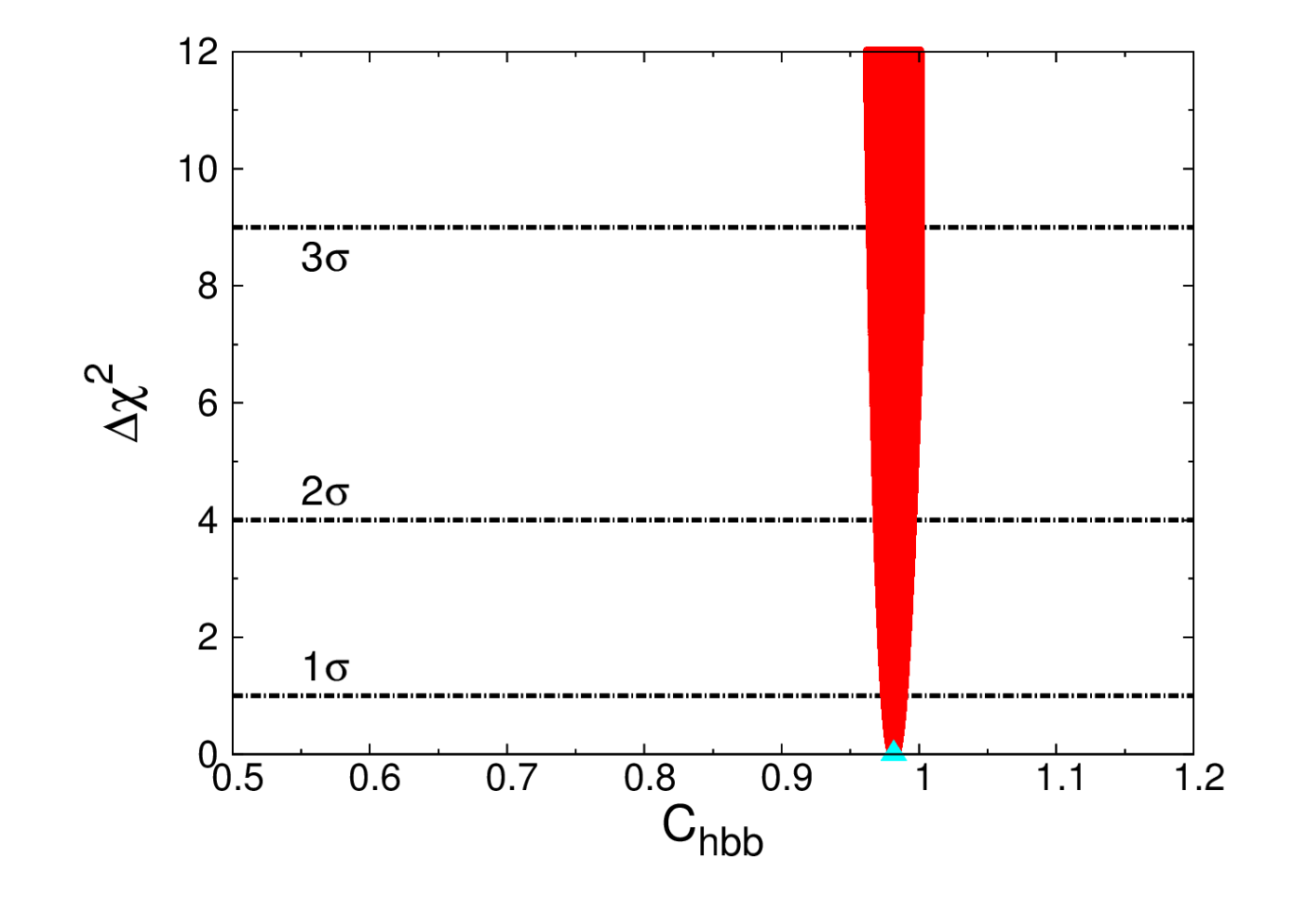
For Fit-1, keeping gb3′′=0g_{b^{\prime\prime}_{3}}=0 can guarantees the flavor-changing coupling (gd​b)L(g^{db})_{L} from Eq. (2.4) to be zero. Therefore the constraints from Bd0​-​B¯d0B^{0}_{d}\text{-}\overline{B}^{0}_{d} mixing, B+→π+​ℓ+​ℓ−B^{+}\to\pi^{+}\ell^{+}\ell^{-}, and B0→μ+​μ−B^{0}\to\mu^{+}\mu^{-} are irrelevant. Both the values of Br(B+→π+​ℓ+​ℓ−)(B^{+}\to\pi^{+}\ell^{+}\ell^{-}) and Br(B0→μ+​μ−)(B^{0}\to\mu^{+}\mu^{-}) are exactly the same as the SM predictions. After performing the fit to the data, Fit-1 gives a minimal chi-square value of χmin2/d.o.f.=63.124/73\chi^{2}_{\rm min}/d.o.f.=63.124/73 and thus a goodness of fit =0.789=0.789. Comparing with the SM fit Fit-1 has a pp-value of 2.5×10−62.5\times 10^{-6} against the SM null hypothesis. It is shown in both Table 2 and Fig. 1 that the best-fit points prefer a non-zero value of gℬ3=±1.177g_{\mathcal{B}_{3}}=\pm 1.177 and gb1′′=±0.335g_{b^{\prime\prime}_{1}}=\pm 0.335 at a level more than 2.5​σ2.5\sigma and 4​σ4\sigma from zero, respectively. Furthermore, the bottom-quark Yukawa coupling deviates from the SM prediction by more than 2​σ2\sigma, and the best-fit points give Ch​b​b=0.98C_{hbb}=0.98, which is about 2% smaller than the SM value. It helps to enhance the overall Higgs signal strengths. In fact, the Higgs signal-strength dataset prefers bottom Yukawa coupling 6% smaller than the SM value Cheung:2019pkj. Since the RbEXPR^{\rm EXP}_{b} was quite precisely measured and consistent with the SM prediction, the deviation of the bottom-Yukawa coupling cannot exceed more than a couple of percent. From the (𝒱L15,𝒱R34)(\mathcal{V}_{\rm L15},\mathcal{V}_{\rm R34}) panel of Fig. 1, since 𝒱L15≃s15L∝gb1′′\mathcal{V}_{\rm L15}\simeq s^{L}_{15}\propto g_{b^{\prime\prime}_{1}} and 𝒱R34≃s34R∝gℬ3\mathcal{V}_{\rm R34}\simeq s^{R}_{34}\propto g_{\mathcal{B}_{3}}, it does not show correlation between gℬ3g_{\mathcal{B}_{3}} and gb1′′g_{b^{\prime\prime}_{1}}. In the (𝒱R​34,Δ​S)(\mathcal{V}_{R34},\Delta S) and (𝒱R​34,Δ​T)(\mathcal{V}_{R34},\Delta T) panels, they show that the best-fit regions are consistent with the oblique parameters from electroweak precision measurements.

Refer to caption
Refer to caption
Refer to caption
Refer to caption
Refer to caption
Refer to caption
Figure 1: Fit-1: the best fit (cyan triangle) gives χmin2=63.124\chi^{2}_{\rm min}=63.124. The contour panels show regions for Δ​χ2≤2.3\Delta\chi^{2}\leq 2.3 (red), 5.995.99 (green), and 11.8311.83 (blue) above the minimum.

In Fit-2, both couplings gb1′′g_{b^{\prime\prime}_{1}} and gb3′′g_{b^{\prime\prime}_{3}} can vary from zero. In this case, according to Eq. (2.4), flavor-changing coupling (gd​b)L(g^{db})_{L} is induced and therefore is constrained B+→π+​ℓ+​ℓ−B^{+}\to\pi^{+}\ell^{+}\ell^{-} and B0→μ+​μ−B^{0}\to\mu^{+}\mu^{-} (Bd0​-​B¯d0B^{0}_{d}\text{-}\bar{B}^{0}_{d} mixing is not included in any of the fits.) In Fig.2 for Fit-2a, which has not included these flavor-changing constraints in the global fit, it allows both couplings gb1′′g_{b^{\prime\prime}_{1}} and gb3′′g_{b^{\prime\prime}_{3}} to significantly deviate from zero. Indeed, we see that the best-fit points prefer gℬ3=±1.651g_{\mathcal{B}_{3}}=\pm 1.651 and gb3′′=±0.614g_{b^{\prime\prime}_{3}}=\pm 0.614, and (s34R)2≃5​(s35L)2(s^{R}_{34})^{2}\simeq 5(s^{L}_{35})^{2} are correlated in (𝒱L​35,𝒱R​34)(\mathcal{V}_{L35},\mathcal{V}_{R34}) panel. This is in accordance with our discussion at end of subsection 3.2, where the VLQs contributions to RbR_{b} cancel among themselves, meanwhile 𝒜F​Bb{\cal A}^{b}_{FB} anomaly is explained by (gb)L(g^{b})_{L}. Since the VLQs contributions to RbR_{b} are canceled, the bottom-Yukawa coupling now is allowed to deviate from the SM by more than 6%, and the best-fit points give Ch​b​b=0.96C_{hbb}=0.96, which deviates form the SM prediction by more than 3​σ3\sigma. Hence, Fit-2a can further lower the minimal chi-square than Fit-1, and gives χmin2/d.o.f.=59.185/70\chi^{2}_{\rm min}/d.o.f.=59.185/70 and thus a goodness of fit equals to 0.8180.818. Unfortunately, there exist constraints from Bd0​-​B¯d0B^{0}_{d}\text{-}\bar{B}^{0}_{d} mixing, B+→π+​ℓ+​ℓ−B^{+}\to\pi^{+}\ell^{+}\ell^{-} and B0→μ+​μ−B^{0}\to\mu^{+}\mu^{-}, which will restrict simultaneously large non-zero values of gb1′′g_{b^{\prime\prime}_{1}} and gb3′′g_{b^{\prime\prime}_{3}}. In order to study the effects from those B physics constraints, we further include both B+→π+​ℓ+​ℓ−B^{+}\to\pi^{+}\ell^{+}\ell^{-} and B0→μ+​μ−B^{0}\to\mu^{+}\mu^{-} in the Fit-2b.

Refer to caption
Refer to caption
Refer to caption
Refer to caption
Refer to caption
Refer to caption
Refer to caption
Refer to caption
Refer to caption
Refer to caption
Refer to caption
Refer to caption
Figure 2: Fit-2a: the best fit (cyan triangle) gives χmin2=59.185\chi^{2}_{\rm min}=59.185. In Ud​b​-​Δ​χ2U_{db}\text{-}\Delta\chi^{2} panel, the hatched region is excluded by Bd0​-​B¯d0B^{0}_{d}\text{-}\overline{B}^{0}_{d} mixing. The contour panels show regions for Δ​χ2≤2.3\Delta\chi^{2}\leq 2.3 (red), 5.995.99 (green), and 11.8311.83 (blue) above the minimum.

In Fig. 3 for Fit-2b, we can understand how the constraints from B+→π+​ℓ+​ℓ−B^{+}\to\pi^{+}\ell^{+}\ell^{-} and B0→μ+​μ−B^{0}\to\mu^{+}\mu^{-} affect the allowed parameter region. In the (gb3′′,Δ​χ2)(g_{b^{\prime\prime}_{3}},\Delta\chi^{2}) panel, the coupling gb3′′g_{b^{\prime\prime}_{3}} is restricted to be small within 3​σ3\sigma, more precisely, it requires |gb3′′|≤0.076|g_{b^{\prime\prime}_{3}}|\leq 0.076. Since gb3′′g_{b^{\prime\prime}_{3}} is restricted close to zero, the best-fit points and the corresponding Ch​b​bC_{hbb} of Fit-2b overlap with Fit-1. In the same panel, we can observe there are two local minima at gb3′′≃±0.6g_{b^{\prime\prime}_{3}}\simeq\pm 0.6 at 4​σ4\sigma, which is correlated to gb1′′≃0g_{b^{\prime\prime}_{1}}\simeq 0 in (gb1′′,Δ​χ2)(g_{b^{\prime\prime}_{1}},\Delta\chi^{2}) panel. From the (Ud​b,Δ​χ2)(U_{db},\Delta\chi^{2}) panel, we know that the flavor constraints from B+→π+​ℓ+​ℓ−B^{+}\to\pi^{+}\ell^{+}\ell^{-} is more stringent than Bd0​-​B¯d0B^{0}_{d}\text{-}\bar{B}^{0}_{d} mixing due to more precise theoretical uncertainty in the former. Around the minimum, we can identify the two-tine fork shape structure, and it is due to the interference between VLQs and SM contributions for B+→π+​ℓ+​ℓ−B^{+}\to\pi^{+}\ell^{+}\ell^{-} from Eq.(3.6). Finally, comparing with B+→π+​ℓ+​ℓ−B^{+}\to\pi^{+}\ell^{+}\ell^{-}, the B0→μ+​μ−B^{0}\to\mu^{+}\mu^{-} gives similar but weaker constraint on (gd​b)L(g^{db})_{L}. We can also find in Table 2 that both the values of Br(B+→π+​ℓ+​ℓ−)(B^{+}\to\pi^{+}\ell^{+}\ell^{-}) and Br(B0→μ+​μ−)(B^{0}\to\mu^{+}\mu^{-}) in Fit-2b are largely reduced by three orders of magnitude compared with Fit-2a. On the other hand, we observe that the value of Br(B+→π+​ℓ+​ℓ−)(B^{+}\to\pi^{+}\ell^{+}\ell^{-}) in Fit-2b is indeed closer to the measurement from LHCb in Eq.(144) than the SM prediction in Eq.(143), because the central value in Eq.(143) is more than 1​σ1\sigma larger than the central value in Eq.(144). Once both theoretical and experimental uncertainties are reduced in the future with almost the same central value in Br(B+→π+​ℓ+​ℓ−)(B^{+}\to\pi^{+}\ell^{+}\ell^{-}), it will be a smoking-gun signature for adding VLQs to the SM.

For discovery prospects of the doublet+singlet VLQs, there are some signatures which can be searched for at the LHC. The VLQs can be pair produced via QCD processes, such as g​g,q​q¯→b′​b′¯,b′′​b′′¯,p′​p′¯gg,q\bar{q}\to b^{\prime}\bar{b^{\prime}},b^{\prime\prime}\bar{b^{\prime\prime}},p^{\prime}\bar{p^{\prime}}. Due to the off-diagonal Yukawa interactions and mixing between VLQs and SM quarks, the VLQs can decay via

b′→Z​b,Z​s,Z​d,h​b,h​s,h​d\displaystyle b^{\prime}\to Zb,Zs,Zd,hb,hs,hd
b′′→W​t,W​c,W​u\displaystyle b^{\prime\prime}\to Wt,Wc,Wu
p′→W​b,W​s,W​d.\displaystyle p^{\prime}\to Wb,Ws,Wd\,.

Here, we assume the mass degeneracy of b′b^{\prime} and p′p^{\prime} from the doublet VLQ to avoid the decay mode b′→p′​Wb^{\prime}\to p^{\prime}W or p′→b′​Wp^{\prime}\to b^{\prime}W. Even though there is slight mass splitting between b′b^{\prime} and p′p^{\prime} of order 𝒪⁡(10)\mathcal{O}(10) GeV due to the mixing effect, the decay p′→b′​Wp^{\prime}\to b^{\prime}W or b′→p′​Wb^{\prime}\to p^{\prime}W can only give very soft leptons or jets, which are very difficult for detection at the LHC.

The decay branching ratios of VLQs, for example, from the best-fit points for Fit-1 and Fit-2b from Table 2 are

BR⁡(b′→Z​b)≃BR⁡(b′→h​b)≃0.5,BR⁡(p′→W​b)≃1.00\displaystyle{\rm BR}(b^{\prime}\to Zb)\simeq{\rm BR}(b^{\prime}\to hb)\simeq 0.5,\ \ {\rm BR}(p^{\prime}\to Wb)\simeq 1.00
BR⁡(b′′→W​c)=0.05,BR⁡(b′′→W​u)=0.95\displaystyle{\rm BR}(b^{\prime\prime}\to Wc)=0.05,\ \ {\rm BR}(b^{\prime\prime}\to Wu)=0.95

, and for Fit-2a,

BR⁡(b′→Z​b)≃BR⁡(b′→h​b)≃0.5,BR⁡(p′→W​b)≃1.00\displaystyle{\rm BR}(b^{\prime}\to Zb)\simeq{\rm BR}(b^{\prime}\to hb)\simeq 0.5,\ \ {\rm BR}(p^{\prime}\to Wb)\simeq 1.00
BR⁡(b′′→W​t)=0.765,BR⁡(b′′→W​c)=0.005,BR⁡(b′′→W​u)=0.230,\displaystyle{\rm BR}(b^{\prime\prime}\to Wt)=0.765,\ \ {\rm BR}(b^{\prime\prime}\to Wc)=0.005,\ \ {\rm BR}(b^{\prime\prime}\to Wu)=0.230\,,

The above relation BR⁡(b′→Z​b)≃BR⁡(b′→h​b){\rm BR}(b^{\prime}\to Zb)\simeq{\rm BR}(b^{\prime}\to hb) comes from the equivalence theorem, in which the longitudinal mode of gauge bosons behaves like the Goldstone boson in the limit Mb′,b′′,p′≫mZ,hM_{b^{\prime},b^{\prime\prime},p^{\prime}}\gg m_{Z,h}. Therefore, one clear signature at the LHC from pair produced b′​b′b^{\prime}b^{\prime} is

b′​b′¯→(b​X)​(b¯​Z)→(b​X)​(b¯​ℓ+​ℓ−),b^{\prime}\bar{b^{\prime}}\to(bX)(\bar{b}Z)\to(bX)(\bar{b}\ell^{+}\ell^{-})\,,

where XX could be either hh or ZZ. Such charged lepton pair(s) plus jets searches have been performed at the 13 TeV LHC  Aaboud:2018saj; Sirunyan:2018qau. Here we roughly estimate the current sensitivity on the lower mass limit of b′b^{\prime}. The event rate with at least one charged lepton pair is

N=σ⁡(p​p→b′​b′¯)×ℒ×ϵN=\sigma(pp\to b^{\prime}\bar{b^{\prime}})\times\mathcal{L}\times\epsilon

where ϵ=0.0028\epsilon=0.0028 taking into account the branching ratios of b′b^{\prime} and Z→ℓ+​ℓ−Z\to\ell^{+}\ell^{-} . Then using ℒ=36.1​fb−1\mathcal{L}=36.1~{\rm fb^{-1}} and requiring N<2N<2, we obtain

σ⁡(p​p→b′​b′¯)≲20​fb.\sigma(pp\to b^{\prime}\bar{b^{\prime}})\lesssim 20~{\rm fb}\,.

By adopting the VLQ pair production cross section, the above upper limit translates into the lower mass limit of Mb′≳1.1​TeVM_{b^{\prime}}\gtrsim 1.1~{\rm TeV}.

Other decay modes of VLQs from pair production have been searched for by ATLAS and CMS Collaborations in Ref. Aaboud:2018wxv; Aaboud:2018pii; Sirunyan:2018omb; Sirunyan:2019sza. The lower mass limits of VLQs are around 1 TeV from these searches. Single VLQ production via the electroweak interaction , which depends on the size of mixing between VLQ and SM quark, was investigated in Ref. Aaboud:2018ifs; Sirunyan:2019xeh. We emphasize the predicted gℬ3g_{\mathcal{B}_{3}} and gb1′′g_{b^{\prime\prime}_{1}} values in Table II all give s34R≃gℬ3​v/(2​M1)≃0.14s^{R}_{34}\simeq g_{\mathcal{B}_{3}}v/(\sqrt{2}M_{1})\simeq 0.14 and s15L≃gb1′′​v/(2​M2)≃0.04s^{L}_{15}\simeq g_{b^{\prime\prime}_{1}}v/(\sqrt{2}M_{2})\simeq 0.04, that can be measured from the single VLQ productions via Z​bZb(W​uWu) fusion and ready to be tested in the near future. For example, the single p′p^{\prime} produced from the W​bWb fusion has been studied by the ATLAS Aaboud:2018ifs. Assuming BR⁡(p′→W​b)=100%{\rm BR}(p^{\prime}\to Wb)=100\% and varying |s34R||s^{R}_{34}| between 0.17 and 0.55, the lower mass limit of p′p^{\prime} can be set from 800 to 1800 GeV.

A distinctive signature of our proposed model from other phenomenological models is the singlet VLQ decay mode b′′→W−​ub^{\prime\prime}\to W^{-}u. On the other hand, most of experimental searches at the LHC were focused on the mixing between VLQs and the third generation quarks. Hence, we stress the searches for the mixing between VLQs and the first generation quarks are also well-motivated in this work. The sizeable or dominant BR⁡(b′′→W−​u){\rm BR}(b^{\prime\prime}\to W^{-}u) can be a distinguishable feature of our scenario.

Refer to caption
Refer to caption
Refer to caption
Refer to caption
Refer to caption
Refer to caption
Refer to caption
Refer to caption
Refer to caption
Refer to caption
Refer to caption
Refer to caption
Figure 3: Fit-2b: the best fit (cyan triangle) gives χmin2=62.275\chi^{2}_{\rm min}=62.275. In Ud​b​-​Δ​χ2U_{db}\text{-}\Delta\chi^{2} panel, the hatched region is excluded by Bd0​-​B¯d0B^{0}_{d}\text{-}\overline{B}^{0}_{d} mixing. The contour panels show regions for Δ​χ2≤2.3\Delta\chi^{2}\leq 2.3 (red), 5.995.99 (green), and 11.8311.83 (blue) above the minimum.
Table 2: The best-fitted values in various fits and the corresponding chi-square per degree of freedom and goodness of fit. The pp-value for each fit hypothesis against the SM null hypothesis is also shown. For the SM, we obtain χ2​(SM)=88.946\chi^{2}(\rm SM)=88.946, χ2/d​o​f=88.946/75\chi^{2}/dof=88.946/75, and corresponding goodness of fit =0.130=0.130. Notice the condition ∑i=d,s,b,b′,b′′|Vu​i|2=1\sum_{i=d,s,b,b^{\prime},b^{{}^{\prime\prime}}}|V_{ui}|^{2}=1 is held during the fitting.

Cases          Fit-1          Fit-2a          Fit-2b Vary gℬ3g_{\mathcal{B}_{3}}, gb1′′g_{b^{\prime\prime}_{1}} Vary gℬ3g_{\mathcal{B}_{3}}, gb1′′g_{b^{\prime\prime}_{1}} Vary gℬ3g_{\mathcal{B}_{3}}, gb1′′g_{b^{\prime\prime}_{1}} Parameters gb3′′g_{b^{\prime\prime}_{3}} gb3′′g_{b^{\prime\prime}_{3}} gℬ3g_{\mathcal{B}_{3}} 1.177−0.225+0.1791.177^{+0.179}_{-0.225} 1.651−0.213+0.1661.651^{+0.166}_{-0.213} 1.176−0.225+0.1791.176^{+0.179}_{-0.225} gb1′′g_{b^{\prime\prime}_{1}} 0.335−0.041+0.0370.335^{+0.037}_{-0.041} 0.339−0.039+0.0350.339^{+0.035}_{-0.039} 0.335−0.041+0.0370.335^{+0.037}_{-0.041} gb3′′g_{b^{\prime\prime}_{3}} 0 0.614−0.149+0.1130.614^{+0.113}_{-0.149} 0.0063−0.0092+0.00490.0063^{+0.0049}_{-0.0092} M1M_{1} [TeV] 1.5 1.5 1.5 M2M_{2} [TeV] 1.5 1.5 1.5 Ch​b​bC_{hbb} 0.982−0.007+0.0060.982^{+0.006}_{-0.007} 0.960−0.009+0.0100.960^{+0.010}_{-0.009} 0.982−0.007+0.0060.982^{+0.006}_{-0.007} χHiggs2\chi^{2}_{\rm Higgs} 52.46 51.38 52.46 𝒜FBb{\cal A}_{\rm FB}^{b} 0.10129 0.09943 0.10129 RbR_{b} 0.21732 0.21676 0.21732 Γtot\Gamma_{\rm tot} 1.7428 1.7415 1.7428 Δ​S\Delta S 0.05 0.11 0.05 Δ​T\Delta T 0.03 0.07 0.03 Br(B+→π+​ℓ+​ℓ−)(B^{+}\to\pi^{+}\ell^{+}\ell^{-}) 7.10×10−97.10\times 10^{-9} 3.87×10−63.87\times 10^{-6} 4.92×10−94.92\times 10^{-9} Br(B0→μ+​μ+)(B^{0}\to\mu^{+}\mu^{+}) 1.45×10−101.45\times 10^{-10} 1.36×10−71.36\times 10^{-7} 0.74×10−100.74\times 10^{-10} χ2/d​o​f\chi^{2}/dof 63.124/73 59.185/70 62.275/72 goodness of fit 0.789 0.818 0.786 pp-value 2.5×10−62.5\times 10^{-6} 2.7×10−62.7\times 10^{-6} 1.2×10−51.2\times 10^{-5}

5 Discussion

We have advocated an extension of the SM with vector-like quarks, including a doublet and a singlet, in aim of alleviating a few experimental anomalies. An urgent one is a severe unitarity violation in the first row of the CKM matrix standing at a level more than 4​σ4\sigma due to a recent more precise evaluation of Vu​dV_{ud} and Vu​sV_{us}. Another one is the long-lasting discrepancy in the forward-backward asymmetry 𝒜FBb{\cal A}_{\rm FB}^{b} in Z→b​b¯Z\to b\bar{b} at LEP. Furthermore, a mild excess in the overall Higgs signal strength appears at about 2​σ2\sigma above the standard model (SM) prediction,

In this work, we have performed global fits of the model under the constraints coming from the unitarity condition of the first row of the CKM matrix, the ZZ-pole observables 𝒜FBb{\cal A}_{\rm FB}^{b}, RbR_{b} and Γhad\Gamma_{\rm had}, Electro-Weak precision observables Δ​S\Delta S and Δ​T\Delta T, BB-meson observables Bd0B_{d}^{0}-B¯d0\overline{B}_{d}^{0} mixing, B+→π+​ℓ+​ℓ−B^{+}\to\pi^{+}\ell^{+}\ell^{-} and B0→μ+​μ−B^{0}\to\mu^{+}\mu^{-}, and direct searches for VLQs at the LHC. We found that the extension with a VLQ doublet and a singlet can improve the fitting to the datasets, especially the improvement to the unitarity condition of the first row of the CKM matrix with two additional entries in the first row.

We offer the following comments before closing.

  1. 1.

    By extending the CKM matrix to 5×55\times 5 with the extra VLQs, the unitarity condition in the first row is fully restored.

  2. 2.

    Without taking into account the B-meson constraints the best-fit (see Fit-2a) can allow the bottom-Yukawa coupling to decrease by about 6%, which can then adequately explain the 2​σ2\sigma excess in the Higgs signal strength. At the same time, it can also account for the 𝒜FBb{\cal A}_{\rm FB}^{b} without upsetting RbR_{b} due to a nontrivial cancellation between two contributions. However, the resulting branching ratios for B+→π+​ℓ+​ℓ−B^{+}\to\pi^{+}\ell^{+}\ell^{-} and B0→μ+​μ−B^{0}\to\mu^{+}\mu^{-} become exceedingly large above the experimental values.

  3. 3.

    However, including the B-meson constraints the allowed parameter space in gb3′′g_{b^{\prime\prime}_{3}} is restricted to be very small due to the presence of the FCNC in ZZ-bb-dd.

  4. 4.

    Last but not least, the extra 5 physical CP phases in 𝐕𝐂𝐊𝐌𝟓×𝟓{\bf V^{5\times 5}_{CKM}} matrix can be a trigger for electroweak baryogenesis. In order to generate the strong first-order electroweak phase transition, one needs to add an extra singlet complex scalar McDonald:1996uz; Branco:1998yk. On the other hand, adding extra Z′Z^{\prime} boson as in the Ref. Rusov:2019ixr would be possible to cancel the FCNC contributions from VLQs. Therefore, a gauge U⁡(1)U(1) extension of our minimal model with a singlet complex scalar may simultaneously alleviate the constraints from B meson observables and explain the matter-antimatter asymmetry of the Universe. However, this extension is beyond the scope of this work and we would like to study this possibility in the future.

Acknowledgment

We thank Jae Sik Lee for initial participation and Chien-Yeah Seng, Michael J. Ramsey-Musolf for the information about the recent determination of Vu​dV_{ud}. W.-Y. K. and P.-Y. T. thank the National Center of Theoretical Sciences, Taiwan, R.O.C. for hospitality. The work of K.C. was supported by the National Science Council of Taiwan under Grants No. MOST-107-2112-M-007-029-MY3.

Appendix A Parameterization of the full 𝐕𝐂𝐊𝐌𝟓×𝟓{\bf V^{5\times 5}_{CKM}} matrix

In this appendix, we display parameterization of the full 𝐕𝐂𝐊𝐌𝟓×𝟓{\bf V^{5\times 5}_{CKM}} matrix in the main text. For the general n×nn\times n CKM matrix, there are n2−(2​n−1)=(n−1)2n^{2}-(2n-1)=(n-1)^{2} physical parameters in the corresponding matrix. For example, there are 3 rotation angles θ12,θ13,θ23\theta_{12},\theta_{13},\theta_{23} and 1 CP phase δ\delta in the 3×33\times 3 CKM matrix of SM. For the 5×55\times 5 CKM matrix, there are 16 physical parameters. Except for the previous 4 parameters in the 3×33\times 3 CKM matrix, we assign the extra 12 parameters as 7 rotation angles θ14,θ15,θ24,θ25,θ34,θ35,θ45\theta_{14},\theta_{15},\theta_{24},\theta_{25},\theta_{34},\theta_{35},\theta_{45} and 5 CP phases ϕ1,ϕ2,ϕ3,ϕ4,ϕ5\phi_{1},\phi_{2},\phi_{3},\phi_{4},\phi_{5} in the 5×55\times 5 CKM matrix.

We first parameterize the original 3×33\times 3 CKM matrix in the usual form

𝐕𝐂𝐊𝐌𝟑×𝟑\displaystyle{\bf V^{3\times 3}_{CKM}} =\displaystyle= (Vu​dVu​sVu​bVc​dVc​sVc​bVt​dVt​sVt​b)\displaystyle\left(\begin{array}[]{ccc}V_{ud}&V_{us}&V_{ub}\\ V_{cd}&V_{cs}&V_{cb}\\ V_{td}&V_{ts}&V_{tb}\\ \end{array}\right)
=\displaystyle= (1000c23s230−s23c23)​(c130s13​e−i​δ010−s13​ei​δ0c13)​(c12s120−s12c120001)\displaystyle\left(\begin{array}[]{ccc}1&0&0\\ 0&c_{23}&s_{23}\\ 0&-s_{23}&c_{23}\\ \end{array}\right)\left(\begin{array}[]{ccc}c_{13}&0&s_{13}e^{-i\delta}\\ 0&1&0\\ -s_{13}e^{i\delta}&0&c_{13}\\ \end{array}\right)\left(\begin{array}[]{ccc}c_{12}&s_{12}&0\\ -s_{12}&c_{12}&0\\ 0&0&1\\ \end{array}\right)
=\displaystyle= (c12​c13s12​c13s13​e−i​δ−s12​c23−c12​s13​s23​ei​δc12​c23−s12​s13​s23​ei​δs23​c13s12​s23−c12​s13​c23​ei​δ−c12​s23−s12​s13​c23​ei​δc23​c13),\displaystyle\left(\begin{array}[]{ccc}c_{12}c_{13}&s_{12}c_{13}&s_{13}e^{-i\delta}\\ -s_{12}c_{23}-c_{12}s_{13}s_{23}e^{i\delta}&c_{12}c_{23}-s_{12}s_{13}s_{23}e^{i\delta}&s_{23}c_{13}\\ s_{12}s_{23}-c_{12}s_{13}c_{23}e^{i\delta}&-c_{12}s_{23}-s_{12}s_{13}c_{23}e^{i\delta}&c_{23}c_{13}\\ \end{array}\right)\,,

with si​j=s​i​n​θi​js_{ij}=sin\theta_{ij} and ci​j=c​o​s​θi​jc_{ij}=cos\theta_{ij} Chau:1984fp. Then we can further parameterize the full 5×55\times 5 CKM matrix based on 𝐕𝐂𝐊𝐌𝟑×𝟑{\bf V^{3\times 3}_{CKM}} as

𝐕𝐂𝐊𝐌𝟓×𝟓\displaystyle{\bf V^{5\times 5}_{CKM}} =\displaystyle= (Vu​dVu​sVu​bVu​b′Vu​b′′Vc​dVc​sVc​bVc​b′Vc​b′′Vt​dVt​sVt​bVt​b′Vt​b′′Vt′​dVt′​sVt′​bVt′​b′Vt′​b′′Vt′′​dVt′′​sVt′′​bVt′′​b′Vt′′​b′′)\displaystyle\left(\begin{array}[]{ccccc}V_{ud}&V_{us}&V_{ub}&V_{ub^{\prime}}&V_{ub^{\prime\prime}}\\ V_{cd}&V_{cs}&V_{cb}&V_{cb^{\prime}}&V_{cb^{\prime\prime}}\\ V_{td}&V_{ts}&V_{tb}&V_{tb^{\prime}}&V_{tb^{\prime\prime}}\\ V_{t^{\prime}d}&V_{t^{\prime}s}&V_{t^{\prime}b}&V_{t^{\prime}b^{\prime}}&V_{t^{\prime}b^{\prime\prime}}\\ V_{t^{\prime\prime}d}&V_{t^{\prime\prime}s}&V_{t^{\prime\prime}b}&V_{t^{\prime\prime}b^{\prime}}&V_{t^{\prime\prime}b^{\prime\prime}}\\ \end{array}\right)
=\displaystyle= (00𝐕𝐂𝐊𝐌𝟑×𝟑00000001000001)​(100000100000100000c45s45​e−i​ϕ5000−s45​ei​ϕ5c45)​(10000010000001000c350s3500−s350c35)\displaystyle\left(\begin{array}[]{ccccc}&&&0&0\\ &{\bf V^{3\times 3}_{CKM}}&&0&0\\ &&&0&0\\ 0&0&0&1&0\\ 0&0&0&0&1\\ \end{array}\right)\left(\begin{array}[]{ccccc}1&0&0&0&0\\ 0&1&0&0&0\\ 0&0&1&0&0\\ 0&0&0&c_{45}&s_{45}e^{-i\phi_{5}}\\ 0&0&0&-s_{45}e^{i\phi_{5}}&c_{45}\\ \end{array}\right)\left(\begin{array}[]{ccccc}1&0&0&0&0\\ 0&1&0&0&0\\ 0&0&0&1&0\\ 0&0&c_{35}&0&s_{35}\\ 0&0&-s_{35}&0&c_{35}\\ \end{array}\right)
⋅\displaystyle\cdot (100000100000c34s34000−s34c34000001)​(100000c2500s25​e−i​ϕ400100000100−s25​ei​ϕ400c25)​(100000c240s24​e−i​ϕ30001000−s24​ei​ϕ30c24000001)\displaystyle\left(\begin{array}[]{ccccc}1&0&0&0&0\\ 0&1&0&0&0\\ 0&0&c_{34}&s_{34}&0\\ 0&0&-s_{34}&c_{34}&0\\ 0&0&0&0&1\\ \end{array}\right)\left(\begin{array}[]{ccccc}1&0&0&0&0\\ 0&c_{25}&0&0&s_{25}e^{-i\phi_{4}}\\ 0&0&1&0&0\\ 0&0&0&1&0\\ 0&-s_{25}e^{i\phi_{4}}&0&0&c_{25}\\ \end{array}\right)\left(\begin{array}[]{ccccc}1&0&0&0&0\\ 0&c_{24}&0&s_{24}e^{-i\phi_{3}}&0\\ 0&0&1&0&0\\ 0&-s_{24}e^{i\phi_{3}}&0&c_{24}&0\\ 0&0&0&0&1\\ \end{array}\right)
⋅\displaystyle\cdot (c15000s15​e−i​ϕ2010000010000010−s15​e−i​ϕ2000c15)​(c1400s14​e−i​ϕ100100000100−s14​ei​ϕ100c14000001)\displaystyle\left(\begin{array}[]{ccccc}c_{15}&0&0&0&s_{15}e^{-i\phi_{2}}\\ 0&1&0&0&0\\ 0&0&1&0&0\\ 0&0&0&1&0\\ -s_{15}e^{-i\phi_{2}}&0&0&0&c_{15}\\ \end{array}\right)\left(\begin{array}[]{ccccc}c_{14}&0&0&s_{14}e^{-i\phi_{1}}&0\\ 0&1&0&0&0\\ 0&0&1&0&0\\ -s_{14}e^{i\phi_{1}}&0&0&c_{14}&0\\ 0&0&0&0&1\\ \end{array}\right)
\displaystyle\,, (219)

where

Vu​d\displaystyle V_{ud} =\displaystyle= c14​(c12​c13​c15−ei​ϕ2​s15​(e−i​δ​c25​s13​s35+e−i​ϕ4​c13​s12​s25))\displaystyle c_{14}\left(c_{12}c_{13}c_{15}-e^{i\phi_{2}}s_{15}\left(e^{-i\delta}c_{25}s_{13}s_{35}+e^{-i\phi_{4}}c_{13}s_{12}s_{25}\right)\right) (220)
−ei​ϕ1​s14​(e−i​ϕ3​s24​(c13​c25​s12−ei⁡(ϕ4−δ)​s13​s25​s35)+e−i​δ​c24​c35​s13​s34)\displaystyle-e^{i\phi_{1}}s_{14}\left(e^{-i\phi_{3}}s_{24}\left(c_{13}c_{25}s_{12}-e^{i(\phi_{4}-\delta)}s_{13}s_{25}s_{35}\right)+e^{-i\delta}c_{24}c_{35}s_{13}s_{34}\right)
Vu​s\displaystyle V_{us} =\displaystyle= c24​(c13​c25​s12−ei⁡(ϕ4−δ)​s13​s25​s35)−ei⁡(ϕ3−δ)​c35​s13​s24​s34\displaystyle c_{24}\left(c_{13}c_{25}s_{12}-e^{i(\phi_{4}-\delta)}s_{13}s_{25}s_{35}\right)-e^{i(\phi_{3}-\delta)}c_{35}s_{13}s_{24}s_{34} (221)
Vu​b\displaystyle V_{ub} =\displaystyle= e−i​δ​c34​c35​s13\displaystyle e^{-i\delta}c_{34}c_{35}s_{13} (222)
Vu​b′\displaystyle V_{ub^{\prime}} =\displaystyle= e−i​ϕ1​s14​(c12​c13​c15−ei​ϕ2​s15​(e−i​δ​c25​s13​s35+e−i​ϕ4​c13​s12​s25))\displaystyle e^{-i\phi_{1}}s_{14}\left(c_{12}c_{13}c_{15}-e^{i\phi_{2}}s_{15}\left(e^{-i\delta}c_{25}s_{13}s_{35}+e^{-i\phi_{4}}c_{13}s_{12}s_{25}\right)\right) (223)
+c14​(e−i​ϕ3​s24​(c13​c25​s12−ei⁡(ϕ4−δ)​s13​s25​s35)+e−i​δ​c24​c35​s13​s34)\displaystyle+c_{14}\left(e^{-i\phi_{3}}s_{24}\left(c_{13}c_{25}s_{12}-e^{i(\phi_{4}-\delta)}s_{13}s_{25}s_{35}\right)+e^{-i\delta}c_{24}c_{35}s_{13}s_{34}\right)
Vu​b′′\displaystyle V_{ub^{\prime\prime}} =\displaystyle= c15​(e−i​δ​c25​s13​s35+e−i​ϕ4​c13​s12​s25)+e−i​ϕ2​c12​c13​s15\displaystyle c_{15}\left(e^{-i\delta}c_{25}s_{13}s_{35}+e^{-i\phi_{4}}c_{13}s_{12}s_{25}\right)+e^{-i\phi_{2}}c_{12}c_{13}s_{15} (224)
Vc​d\displaystyle V_{cd} =\displaystyle= −c14​(c15​(c23​s12+ei​δ​c12​s13​s23)+ei​ϕ2​s15​(c13​c25​s23​s35+e−i​ϕ4​s25​(c12​c23−ei​δ​s12​s13​s23)))\displaystyle-c_{14}\left(c_{15}\left(c_{23}s_{12}+e^{i\delta}c_{12}s_{13}s_{23}\right)+e^{i\phi_{2}}s_{15}\left(c_{13}c_{25}s_{23}s_{35}+e^{-i\phi_{4}}s_{25}\left(c_{12}c_{23}-e^{i\delta}s_{12}s_{13}s_{23}\right)\right)\right) (225)
−ei​ϕ1​s14​(c13​c24​c35​s23​s34+e−i​ϕ3​s24​(c25​(c12​c23−ei​δ​s12​s13​s23)−ei​ϕ4​c13​s23​s25​s35))\displaystyle-e^{i\phi_{1}}s_{14}\left(c_{13}c_{24}c_{35}s_{23}s_{34}+e^{-i\phi_{3}}s_{24}\left(c_{25}\left(c_{12}c_{23}-e^{i\delta}s_{12}s_{13}s_{23}\right)-e^{i\phi_{4}}c_{13}s_{23}s_{25}s_{35}\right)\right)
Vc​s\displaystyle V_{cs} =\displaystyle= c24​(c25​(c12​c23−ei​δ​s12​s13​s23)−ei​ϕ4​c13​s23​s25​s35)−ei​ϕ3​c13​c35​s23​s24​s34\displaystyle c_{24}\left(c_{25}\left(c_{12}c_{23}-e^{i\delta}s_{12}s_{13}s_{23}\right)-e^{i\phi_{4}}c_{13}s_{23}s_{25}s_{35}\right)-e^{i\phi_{3}}c_{13}c_{35}s_{23}s_{24}s_{34} (226)
Vc​b\displaystyle V_{cb} =\displaystyle= c13​c34​c35​s23\displaystyle c_{13}c_{34}c_{35}s_{23} (227)
Vc​b′\displaystyle V_{cb^{\prime}} =\displaystyle= −e−i​ϕ1​s14​(c15​(c23​s12+ei​δ​c12​s13​s23)+ei​ϕ2​s15​(c13​c25​s23​s35+e−i​ϕ4​s25​(c12​c23−ei​δ​s12​s13​s23)))\displaystyle-e^{-i\phi_{1}}s_{14}\left(c_{15}\left(c_{23}s_{12}+e^{i\delta}c_{12}s_{13}s_{23}\right)+e^{i\phi_{2}}s_{15}\left(c_{13}c_{25}s_{23}s_{35}+e^{-i\phi_{4}}s_{25}\left(c_{12}c_{23}-e^{i\delta}s_{12}s_{13}s_{23}\right)\right)\right) (228)
+c14​(c13​c24​c35​s23​s34+e−i​ϕ3​s24​(c25​(c12​c23−ei​δ​s12​s13​s23)−ei​ϕ4​c13​s23​s25​s35))\displaystyle+c_{14}\left(c_{13}c_{24}c_{35}s_{23}s_{34}+e^{-i\phi_{3}}s_{24}\left(c_{25}\left(c_{12}c_{23}-e^{i\delta}s_{12}s_{13}s_{23}\right)-e^{i\phi_{4}}c_{13}s_{23}s_{25}s_{35}\right)\right)
Vc​b′′\displaystyle V_{cb^{\prime\prime}} =\displaystyle= −e−i​ϕ2​s15​(c23​s12+ei​δ​c12​s13​s23)+c15​(c13​c25​s23​s35+e−i​ϕ4​s25​(c12​c23−ei​δ​s12​s13​s23))\displaystyle-e^{-i\phi_{2}}s_{15}\left(c_{23}s_{12}+e^{i\delta}c_{12}s_{13}s_{23}\right)+c_{15}\left(c_{13}c_{25}s_{23}s_{35}+e^{-i\phi_{4}}s_{25}\left(c_{12}c_{23}-e^{i\delta}s_{12}s_{13}s_{23}\right)\right) (229)
Vt​d\displaystyle V_{td} =\displaystyle= c14​(c15​(s12​s23−ei​δ​c12​c23​s13)−ei​ϕ2​s15​(c13​c23​c25​s35−e−i​ϕ4​s25​(c12​s23+ei​δ​c23​s12​s13)))\displaystyle c_{14}\left(c_{15}\left(s_{12}s_{23}-e^{i\delta}c_{12}c_{23}s_{13}\right)-e^{i\phi_{2}}s_{15}\left(c_{13}c_{23}c_{25}s_{35}-e^{-i\phi_{4}}s_{25}\left(c_{12}s_{23}+e^{i\delta}c_{23}s_{12}s_{13}\right)\right)\right) (230)
−ei​ϕ1​s14​(c13​c23​c24​c35​s34−e−i​ϕ3​s24​(c25​(c12​s23+ei​δ​c23​s12​s13)+ei​ϕ4​c13​c23​s25​s35))\displaystyle-e^{i\phi_{1}}s_{14}\left(c_{13}c_{23}c_{24}c_{35}s_{34}-e^{-i\phi_{3}}s_{24}\left(c_{25}\left(c_{12}s_{23}+e^{i\delta}c_{23}s_{12}s_{13}\right)+e^{i\phi_{4}}c_{13}c_{23}s_{25}s_{35}\right)\right)
Vt​s\displaystyle V_{ts} =\displaystyle= −c24​(c25​(c12​s23+ei​δ​c23​s12​s13)+ei​ϕ4​c13​c23​s25​s35)−ei​ϕ3​c13​c23​c35​s24​s34\displaystyle-c_{24}\left(c_{25}\left(c_{12}s_{23}+e^{i\delta}c_{23}s_{12}s_{13}\right)+e^{i\phi_{4}}c_{13}c_{23}s_{25}s_{35}\right)-e^{i\phi_{3}}c_{13}c_{23}c_{35}s_{24}s_{34} (231)
Vt​b\displaystyle V_{tb} =\displaystyle= c13​c23​c34​c35\displaystyle c_{13}c_{23}c_{34}c_{35} (232)
Vt​b′\displaystyle V_{tb^{\prime}} =\displaystyle= e−i​ϕ1​s14​(c15​(s12​s23−ei​δ​c12​c23​s13)−ei​ϕ2​s15​(c13​c23​c25​s35−e−i​ϕ4​s25​(c12​s23+ei​δ​c23​s12​s13)))\displaystyle e^{-i\phi_{1}}s_{14}\left(c_{15}\left(s_{12}s_{23}-e^{i\delta}c_{12}c_{23}s_{13}\right)-e^{i\phi_{2}}s_{15}\left(c_{13}c_{23}c_{25}s_{35}-e^{-i\phi_{4}}s_{25}\left(c_{12}s_{23}+e^{i\delta}c_{23}s_{12}s_{13}\right)\right)\right) (233)
+c14​(c13​c23​c24​c35​s34−e−i​ϕ3​s24​(c25​(c12​s23+ei​δ​c23​s12​s13)−ei​ϕ4​c13​c23​s25​s35))\displaystyle+c_{14}\left(c_{13}c_{23}c_{24}c_{35}s_{34}-e^{-i\phi_{3}}s_{24}\left(c_{25}\left(c_{12}s_{23}+e^{i\delta}c_{23}s_{12}s_{13}\right)-e^{i\phi_{4}}c_{13}c_{23}s_{25}s_{35}\right)\right)
Vt​b′′\displaystyle V_{tb^{\prime\prime}} =\displaystyle= e−i​ϕ2​s15​(s12​s23−ei​δ​c12​c23​s13)+c15​(c13​c23​c25​s35−e−i​ϕ4​s25​(c12​s23+ei​δ​c23​s12​s13))\displaystyle e^{-i\phi_{2}}s_{15}\left(s_{12}s_{23}-e^{i\delta}c_{12}c_{23}s_{13}\right)+c_{15}\left(c_{13}c_{23}c_{25}s_{35}-e^{-i\phi_{4}}s_{25}\left(c_{12}s_{23}+e^{i\delta}c_{23}s_{12}s_{13}\right)\right) (234)
Vt′​d\displaystyle V_{t^{\prime}d} =\displaystyle= −ei⁡(ϕ2−ϕ5)​c14​c25​c35​s15​s45−ei​ϕ1​s14​(c24​(c34​c45−e−i​ϕ5​s34​s35​s45)−ei⁡(ϕ4−ϕ3−ϕ5)​c35​s24​s25​s45)\displaystyle-e^{i(\phi_{2}-\phi_{5})}c_{14}c_{25}c_{35}s_{15}s_{45}-e^{i\phi_{1}}s_{14}\left(c_{24}\left(c_{34}c_{45}-e^{-i\phi_{5}}s_{34}s_{35}s_{45}\right)-e^{i(\phi_{4}-\phi_{3}-\phi_{5})}c_{35}s_{24}s_{25}s_{45}\right) (235)
Vt′​s\displaystyle V_{t^{\prime}s} =\displaystyle= −ei⁡(ϕ4−ϕ5)​c24​c35​s25​s45−ei​ϕ3​s24​(c34​c45−e−i​ϕ5​s34​s35​s45)\displaystyle-e^{i(\phi_{4}-\phi_{5})}c_{24}c_{35}s_{25}s_{45}-e^{i\phi_{3}}s_{24}\left(c_{34}c_{45}-e^{-i\phi_{5}}s_{34}s_{35}s_{45}\right) (236)
Vt′​b\displaystyle V_{t^{\prime}b} =\displaystyle= −c45​s34−e−i​ϕ5​c34​s35​s45\displaystyle-c_{45}s_{34}-e^{-i\phi_{5}}c_{34}s_{35}s_{45} (237)
Vt′​b′\displaystyle V_{t^{\prime}b^{\prime}} =\displaystyle= c14​(c24​(c34​c45−e−i​ϕ5​s34​s35​s45)−ei⁡(ϕ4−ϕ3−ϕ5)​c35​s24​s25​s45)−ei⁡(ϕ2−ϕ1−ϕ5)​c25​c35​s14​s15​s45\displaystyle c_{14}\left(c_{24}\left(c_{34}c_{45}-e^{-i\phi_{5}}s_{34}s_{35}s_{45}\right)-e^{i(\phi_{4}-\phi_{3}-\phi_{5})}c_{35}s_{24}s_{25}s_{45}\right)-e^{i(\phi_{2}-\phi_{1}-\phi_{5})}c_{25}c_{35}s_{14}s_{15}s_{45} (238)
Vt′​b′′\displaystyle V_{t^{\prime}b^{\prime\prime}} =\displaystyle= e−i​ϕ5​c15​c25​c35​s45\displaystyle e^{-i\phi_{5}}c_{15}c_{25}c_{35}s_{45} (239)
Vt′′​d\displaystyle V_{t^{\prime\prime}d} =\displaystyle= −ei​ϕ2​c14​c25​c35​c45​s15+ei​ϕ1​s14​(c24​(c45​s34​s35+ei​ϕ5​c34​s45)+ei⁡(ϕ4−ϕ3)​c35​c45​s24​s25)\displaystyle-e^{i\phi_{2}}c_{14}c_{25}c_{35}c_{45}s_{15}+e^{i\phi_{1}}s_{14}\left(c_{24}\left(c_{45}s_{34}s_{35}+e^{i\phi_{5}}c_{34}s_{45}\right)+e^{i(\phi_{4}-\phi_{3})}c_{35}c_{45}s_{24}s_{25}\right) (240)
Vt′′​s\displaystyle V_{t^{\prime\prime}s} =\displaystyle= −ei​ϕ4​c24​c35​c45​s25+ei​ϕ3​s24​(c45​s34​s35+ei​ϕ5​c34​s45)\displaystyle-e^{i\phi_{4}}c_{24}c_{35}c_{45}s_{25}+e^{i\phi_{3}}s_{24}\left(c_{45}s_{34}s_{35}+e^{i\phi_{5}}c_{34}s_{45}\right) (241)
Vt′′​b\displaystyle V_{t^{\prime\prime}b} =\displaystyle= −c34​c45​s35+ei​ϕ5​s34​s45\displaystyle-c_{34}c_{45}s_{35}+e^{i\phi_{5}}s_{34}s_{45} (242)
Vt′′​b′\displaystyle V_{t^{\prime\prime}b^{\prime}} =\displaystyle= −c14​(c24​(c45​s34​s35+ei​ϕ5​c34​s45)+ei⁡(ϕ4−ϕ3)​c35​c45​s24​s25)−ei⁡(ϕ2−ϕ1)​c25​c35​c45​s14​s15\displaystyle-c_{14}\left(c_{24}\left(c_{45}s_{34}s_{35}+e^{i\phi_{5}}c_{34}s_{45}\right)+e^{i(\phi_{4}-\phi_{3})}c_{35}c_{45}s_{24}s_{25}\right)-e^{i(\phi_{2}-\phi_{1})}c_{25}c_{35}c_{45}s_{14}s_{15} (243)
Vt′′​b′′\displaystyle V_{t^{\prime\prime}b^{\prime\prime}} =\displaystyle= c15​c25​c35​c45\displaystyle c_{15}c_{25}c_{35}c_{45} (244)

Notice that there is some freedom to arrange the positions of extra 5 CP phases in those matrices. We assign there is no CP phase in the rotation matrices of θ34\theta_{34} and θ35\theta_{35} in this study. On the other hand, since we don’t involve the vector-like up-type quarks t′,t′′t^{\prime},t^{\prime\prime} inside the model, only the measurable 3×53\times 5 sub-matrix of 𝐕𝐂𝐊𝐌𝟓×𝟓{\bf V^{5\times 5}_{CKM}} is corresponding for our study here.

References

  • (1) N. Cabibbo, Phys. Rev. Lett. 10, 531 (1963). doi:10.1103/PhysRevLett.10.531
  • (2) M. Kobayashi and T. Maskawa, Prog. Theor. Phys. 49, 652 (1973). doi:10.1143/PTP.49.652
  • (3) J. C. Hardy and I. S. Towner, Phys. Rev. C 91, no. 2, 025501 (2015), [arXiv:1411.5987 [nucl-ex]].
  • (4) B. Belfatto, R. Beradze and Z. Berezhiani, arXiv:1906.02714 [hep-ph].
  • (5) C. Y. Seng, M. Gorchtein, H. H. Patel and M. J. Ramsey-Musolf, Phys. Rev. Lett. 121, no. 24, 241804 (2018), [arXiv:1807.10197 [hep-ph]].
  • (6) C. Y. Seng, M. Gorchtein and M. J. Ramsey-Musolf, Phys. Rev. D 100, no. 1, 013001 (2019) doi:10.1103/PhysRevD.100.013001 [arXiv:1812.03352 [nucl-th]].
  • (7) C. Y. Seng and U. G. Meißner, Phys. Rev. Lett. 122, no. 21, 211802 (2019) doi:10.1103/PhysRevLett.122.211802 [arXiv:1903.07969 [hep-ph]].
  • (8) M. Moulson, PoS CKM 2016, 033 (2017) doi:10.22323/1.291.0033 [arXiv:1704.04104 [hep-ex]].
  • (9) M. Tanabashi et al. [Particle Data Group], Phys. Rev. D 98, no. 3, 030001 (2018). doi:10.1103/PhysRevD.98.030001
  • (10) A. M. Coutinho, A. Crivellin and C. A. Manzari, arXiv:1912.08823 [hep-ph].
  • (11) Y. S. Amhis et al. [HFLAV Collaboration], arXiv:1909.12524 [hep-ex].
  • (12) A. Lusiani, SciPost Phys. Proc. 1, 001 (2019) doi:10.21468/SciPostPhysProc.1.001 [arXiv:1811.06470 [hep-ex]].
  • (13) G. Aad et al. [ATLAS Collaboration], Phys. Lett. B 716, 1 (2012) doi:10.1016/j.physletb.2012.08.020 [arXiv:1207.7214 [hep-ex]].
  • (14) S. Chatrchyan et al. [CMS Collaboration], Phys. Lett. B 716, 30 (2012) doi:10.1016/j.physletb.2012.08.021 [arXiv:1207.7235 [hep-ex]].
  • (15) The ATLAS collaboration [ATLAS Collaboration], ATLAS-CONF-2018-031.
  • (16) A. M. Sirunyan et al. [CMS Collaboration], Eur. Phys. J. C 79, no. 5, 421 (2019), [arXiv:1809.10733 [hep-ex]].
  • (17) K. Cheung, W. Y. Keung, J. S. Lee and P. Y. Tseng, Phys. Lett. B 798, 134983 (2019), [arXiv:1901.05626 [hep-ph]].
  • (18) D. Choudhury, T. M. P. Tait and C. E. M. Wagner, Phys. Rev. D 65, 053002 (2002) doi:10.1103/PhysRevD.65.053002 [hep-ph/0109097].
  • (19) B. Batell, S. Gori and L. T. Wang, JHEP 1301, 139 (2013) doi:10.1007/JHEP01(2013)139 [arXiv:1209.6382 [hep-ph]].
  • (20) J. A. Aguilar-Saavedra, R. Benbrik, S. Heinemeyer and M. Pérez-Victoria, Phys. Rev. D 88, no. 9, 094010 (2013) doi:10.1103/PhysRevD.88.094010 [arXiv:1306.0572 [hep-ph]].
  • (21) C. Y. Chen, S. Dawson and E. Furlan, Phys. Rev. D 96, no. 1, 015006 (2017) doi:10.1103/PhysRevD.96.015006 [arXiv:1703.06134 [hep-ph]].
  • (22) ATLAS, CMS, G. Aad et al., JHEP 08, 045 (2016), 1606.02266.
  • (23) K. Cheung, J. S. Lee and P. Y. Tseng, JHEP 1909, 098 (2019), [arXiv:1810.02521 [hep-ph]].
  • (24) L. Lavoura and J. P. Silva, Phys. Rev. D 47, 2046 (1993). doi:10.1103/PhysRevD.47.2046
  • (25) M. Carena, E. Ponton, J. Santiago and C. E. M. Wagner, Nucl. Phys. B 759, 202 (2006) doi:10.1016/j.nuclphysb.2006.10.012 [hep-ph/0607106].
  • (26) C. Anastasiou, E. Furlan and J. Santiago, Phys. Rev. D 79, 075003 (2009) doi:10.1103/PhysRevD.79.075003 [arXiv:0901.2117 [hep-ph]].
  • (27) D. Silverman, Phys. Rev. D 58, 095006 (1998), [hep-ph/9806489].
  • (28) J. A. Aguilar-Saavedra, Phys. Rev. D 67, 035003 (2003), [hep-ph/0210112].
  • (29) F.J. Gilman, Annu. Rev. Nucl. Part. Sci. 1990 40, 213-38.
  • (30) W. S. Hou, M. Kohda and F. Xu, Phys. Rev. D 90, no. 1, 013002 (2014), [arXiv:1403.7410 [hep-ph]].
  • (31) A. V. Rusov, arXiv:1911.12819 [hep-ph].
  • (32) A. K. Alok, S. Banerjee, D. Kumar and S. Uma Sankar, Nucl. Phys. B 906, 321 (2016) doi:10.1016/j.nuclphysb.2016.03.012 [arXiv:1402.1023 [hep-ph]].
  • (33) R. Aaij et al. [LHCb Collaboration], Phys. Rev. Lett. 122, no. 19, 191801 (2019) doi:10.1103/PhysRevLett.122.191801 [arXiv:1903.09252 [hep-ex]].
  • (34) A. Abdesselam et al. [Belle Collaboration], arXiv:1904.02440 [hep-ex].
  • (35) R. Aaij et al. [LHCb Collaboration], JHEP 1510, 034 (2015), [arXiv:1509.00414 [hep-ex]].
  • (36) M. Aaboud et al. [ATLAS Collaboration], Phys. Rev. Lett. 121, no. 21, 211801 (2018) doi:10.1103/PhysRevLett.121.211801 [arXiv:1808.02343 [hep-ex]].
  • (37) A. M. Sirunyan et al. [CMS Collaboration], Eur. Phys. J. C 79, no. 4, 364 (2019) doi:10.1140/epjc/s10052-019-6855-8 [arXiv:1812.09768 [hep-ex]].
  • (38) A. M. Sirunyan et al. [CMS Collaboration], arXiv:1906.11903 [hep-ex].
  • (39) The ATLAS collaboration [ATLAS Collaboration], ATLAS-CONF-2018-024.
  • (40) A. M. Sirunyan et al. [CMS Collaboration], Phys. Lett. B 779, 82 (2018) doi:10.1016/j.physletb.2018.01.077 [arXiv:1710.01539 [hep-ex]].
  • (41) M. Aaboud et al. [ATLAS Collaboration], JHEP 1905, 164 (2019) doi:10.1007/JHEP05(2019)164 [arXiv:1812.07343 [hep-ex]].
  • (42) ATLAS, M. Aaboud et al., Phys. Rev. D98, 092005 (2018), 1808.01771.
  • (43) CMS, A. M. Sirunyan et al., JHEP 08, 177 (2018), 1805.04758.
  • (44) ATLAS, M. Aaboud et al., Phys. Rev. D98, 112010 (2018), 1806.10555.
  • (45) A. M. Sirunyan et al. [CMS Collaboration], JHEP 2001, 036 (2020), [arXiv:1909.04721 [hep-ex]].
  • (46) L. L. Chau and W. Y. Keung, Phys. Rev. Lett. 53, 1802 (1984).
  • (47) J. McDonald, Phys. Rev. D 53, 645 (1996). doi:10.1103/PhysRevD.53.645
  • (48) G. C. Branco, D. Delepine, D. Emmanuel-Costa and F. R. Gonzalez, Phys. Lett. B 442, 229 (1998) doi:10.1016/S0370-2693(98)01253-2 [hep-ph/9805302].