This manuscript was compiled on August 11, 2026
Moiré magnetsDOI: www.pnas.org/cgi/doi/10.1073/pnas.XXXXXXXXXX
Abstract
We introduce a general framework to study moiré structures of two-dimensional Van der Waals magnets using continuum field theory. The formalism eliminates quasiperiodicity and allows a full understanding of magnetic structures and their excitations. In particular, we analyze in detail twisted bilayers of Néel antiferromagnets on the honeycomb lattice. A rich phase diagram with non-collinear twisted phases is obtained, and spin waves are further calculated. Direct extensions to zig-zag antiferromagnets and ferromagnets are also presented. We anticipate the results and formalism presented to lead to a broad range of applications to both fundamental research and experiments.
Keywords:
Moiré Van der Waals magnets Hydrodynamics Twisted bilayerE-mail: balents@kitp.ucsb.edu
The wealth of new phenomena revealed in incommensurate layered structures of graphene and other two dimensional semi-conductors and semi-metals have sparked major efforts in the study of electronic physics atop moiré patterns. The materials from which these structures are made, Van der Waals (VdW) solids, come in many varieties, inspiring a nascent field going well beyond grapheneNovoselovReview. In particular, a growing family of VdW magnets are being explored both for their magnetism directly as well as for the interplay of that magnetism with electronics BurchReview. Two dimensional magnets are of particular interest for the fluctuation effects inherent to them. For example, the Mermin-Wagner theorem MerminWagner proves that a strictly two-dimensional magnet with Heisenberg or XY symmetry cannot show long-range order at any non-zero temperature. Exotic quantum phases of magnets, e.g. quantum spin liquids, are widely expected to be more prevalent in two dimensions0034-4885-80-1-016502.
In this paper, we introduce a framework to study moiré structures of two dimensional magnets, under assumptions which are widely applicable and achievable in VdW systems. We present a general methodology to derive continuum models for incommensurate/twisted/strained multilayers including the effects of interlayer coupling, obviating the need to consider thousands or tens of thousands of lattice sites/spins with complicated local environments. We illustrate the method with detailed calculations for the case of a twisted bilayer of two-sublattice Néel antiferromagnets on the honeycomb lattice, a situation realized in MnPS3 Ouvrard; LeFlem; Kurosawa, MnPSe3 LeFlem, and also discuss applications to honeycomb lattice antiferromagnets with zig-zag magnetic order (as in FePS3 Kurosawa, CoPS3 Ouvrard, NiPS3 OuvrardThesis, see Brec for a review) and to the honeycomb lattice ferromagnet CrI3 Huang. We show that twisting these magnets leads to controllable emergent non-collinear spin textures (despite the fact that the parent materials all exhibit collinear ordering), and a rich spectrum of magnonic subbands.
Now we turn to the exposition of the problem and approach, which we illustrate as we go for the simplest case of a two-sublattice Néel order on the honeycomb lattice. First we detail the assumptions under which a continuum description is possible. We consider structures built from two dimensional magnets with long range magnetic order at zero temperature, and assume that the inter-layer exchange interactions are weak compared to the intra-layer exchange , i.e. . Additionally, we assume that the lattice in each layer may be regarded as a deformed version of a parent structure shared by all layers. Each layer is described by a displacement field in Eulerian coordinates:
| (1) |
where and are the deformed and original positions, respectively, of points in layer . The displacement field of each layer need not be uniform or small but its gradients should be small, i.e. . For uniform layers, this allows any long-period moiré structure, i.e. for which the period of the moiré pattern is large compared to the magnetic unit cell. For two identical but twisted layers, it corresponds to the case of a small twist angle, . This construction is directly analogous to the procedure to build the continuum model of twisted bilayer graphenebistritzer2011moire following the recent derivation in Ref.10.21468/SciPostPhys.7.4.048 which is valid under nearly identical assumptions.
In this situation the interlayer couplings and the displacement gradients are small perturbations on the intrinsic magnetism of the layers, and therefore have signficant effects only at low energies. This allows a continuum representation of the magnetism of each layer in terms of its low energy modes: space-time fluctuations of the order parameters. The order parameter of the two sublattice antiferromagnet is a Néel vector with fixed length , and its low energy dynamics for an isolated undeformed layer is described by the non-linear sigma model with the Lagrange density
| (2) |
where is the spin stiffness, is the spin-wave velocity, and is a uniaxial anisotropy with signifying Ising-like and XY-like anti-ferromagnetism. For MnPS3, there is weak Ising-like anisotropy Wildes so ( is the area of the 2d unit cell). Such smallness (but not the sign) of the anisotropy is common for third row transition metal magnets.
Next we consider the first order effects of displacement gradients upon the intra-layer terms in (2). As in Ref. 10.21468/SciPostPhys.7.4.048, such terms arise from pure geometry – i.e. carrying out the coordinate transformation from to defined in (1) – and from strain-induced changes in energetics. Taking them together, the leading corrections to (2) are
| (3) | ||||
where are dimensionless constants and is the strain field in layer . For simplicity we assumed that spin-orbit effects (e.g. anisotropy ) are small and hence that deformation terms in (3) are SU(2) invariant: anisotropic deformation terms must be small in both spin-orbit coupling and in displacement gradients, and hence are neglected.
Next we turn to the inter-layer coupling terms. By locality and translational symmetry, it is generally of the form
| (4) |
where is a function with the periodicity of the undeformed Bravais lattice. Due to the smallness of , we neglect corrections proportional to displacement gradients in (4). Generally can be expanded in a Fourier series, and well-approximated by a small number of harmonics. We obtain a specific form by considering local coupling of the spin densities in the two layers. Using the symmetries of the honeycomb lattice, the minimal Fourier expansion of the spin density of a single layer contains the three minimal reciprocal lattice vectors ,
| (5) |
where measures the size of the ordered moment, and we define the origin at the center of a hexagon. Taking the product and applying trigonometric identities to extract the terms which vary slowly on the lattice scale (rapidly varying components do not contribute at low energy) gives the form of (4), with
| (6) |
where the constant is proportional to the inter-layer exchange and . Physically, (6) captures the fact that e.g. for intrinsically ferromagnetic exchange , the preferred relative orientation of the A sublattice spins of the two layers is parallel for AA stacking but anti-parallel for AB and BA stackings.
The full Lagrange density captures the low energy physics of a bilayer with arbitrary deformations of the two layers. We now specialize to the case of a rigid twist of the two layers by a relative angle : . In this case the strain vanishes, and one finds the full Lagrangian is
| (7) |
where
| (8) |
is the classical energy density. Here the coupling function
| (9) |
and are the reciprocal lattice vectors of the moiré superlattice.
Equations (7)-(9) form the basis for an analysis of the magnetic structure on the moiré scale, as well as for the magnon excitations above them. The magnetic ground state is obtained as the variational minimum of . Owing to the sign change of , the problem is frustrated: the Néel vectors of the two layers wish to be parallel in some regions and antiparallel in others, forcing them to develop gradients within the plane – the representation in the continuum of incompletely satisfied in-plane bonds. We find that the optimal classical solution is coplanar but not necessarily collinear (see the Supporting Information for a complete weak coupling analysis), and without loss of generality we can take the spins to lie in the x-z plane: . The formulae are simplified by forming symmetric and antisymmetric combinations, , , and adopting dimensionless coordinates , with the moiré wavevector. Then the dimensionless energy density becomes, up to an additive constant
| (10) |
Here we introduced the dimensionless parameters
| (11) |
and , where are unit vectors. We can obtain partial differential equations for the phase angles by applying calculus of variations to (10):
| (12) | ||||
| (13) |
We must find the solutions of the saddle point equations which minimize the integral of . There is always a trivial solution with , which corresponds to the Ising limit of aligned or counter-aligned spins. Nontrivial solutions with potentially lower energies will be discussed in different limits below. We first focus on the case .
For , corresponding to large angles, the gradient terms in the Hamiltonian dominate and the solution is nearly constant. Perturbation theory with fixed gives a nontrivial solution
| (14) | ||||
with , and where is a constant given in Sec. C of the Supporting Information. In this twisted solution, tends to imitate the sign of , to gain energy from the potential term. This change of , however, will need to be balanced against the energy penalty due to the kinetic term. Comparing the energy of the twisted solution with the trivial one, we see that it has a lower energy for , i.e., whenever it exists; in this limit, at , the system undergoes a continuous transition to the collinear phase. More details can be found in the Supporting Information.
For small angles, on the other hand, ; in this limit, we first consider small values of ; the potential term in (10) dominates and the energy is minimized by choosing or almost everywhere, so that , which means the order parameter vectors in the two layers are locally parallel or antiparallel. At small values of , it is preferred for to take a constant value and, since the total area with negative is larger than the positive area, is chosen; this solution lies in the same phase as that of the twisted solution found for above, that also showed the property ; we call this phase twisted-s. The twisted-s solution obviously breaks the U(1) symmetry of spin rotations about the axis of spin space, but it retains an Ising symmetry under interchanging layers and reflecting spin . One may check that is odd under this symmetry.
Interestingly however, one can further check that in the same limit of , above some order-one value of , another twisted solution becomes more energetically favored. It belongs to what we call a twisted-a phase, where is no longer constant and actually shows a twisted pattern similar to that of , such that exhibits spatial variations following those of (see the Supporting Information for details). This implies a non-zero value for so that the twisted-a phase spontaneously breaks the aforementioned Ising symmetry. The value of increases smoothly from zero on entering the twisted-a phase from the twisted-s one, consistent with the expected continuous behavior of an Ising transition (treated at mean-field level by the saddle point analysis).
One can finally study the limit. The twisted-a solution in this limit, which is the lowest energy nontrivial solution, requires along with to also have the values or almost everywhere so that matches the sign of ; this means simply that the vectors align or counter-align along the axis almost everywhere. The order parameter rotations occur in a narrow domain wall centered on the zeros of , i.e. forming a closed almost circular loop in the middle of the unit cell. This domain wall costs an energy proportional to its length; as a result of this energy penalty, the twisted-a phase gives way to the collinear phase when the energy gain from the twist is exceeded by the domain wall energy. In order to study this competition, we assume that such transition occurs when , which we later check is self-consistent. The widths and (in dimensionless distance normal to the domain wall) over which and wind are determined by the balance of the gradient terms and the corresponding potential terms. This gives in this limit and an energy cost per unit length of the wall of . Now the bulk energy gain of the twisted state is simply proportional to , so we obtain the result that the twist collapses when . This treatment is valid since under these conditions (we did not determine the multiplicative order one constant in this inequality). Note that the transition between the collinear and twisted-a phase is a “level crossing” between two distinct and disconnected saddle points; consequently it corresponds to a first order transition, and the first derivatives of the energy are discontinuous across this boundary. A tricritical point separates the two continuous transitions from this first order one.
To summarize, we find three different phases for , two of which correspond to twisted solutions. The transition between the two twisted phases happens at some of order , when the phase boundary is crossed in the large limit; the twisted phases collapse on the other hand when in the limit (twisted-s to Ising transition) and when in the limit (twisted-a to Ising transition). We sketch a phase diagram in Fig. 1 from the numerical solution to (12), (13) in Fig. 1, which is consistent with and in fact interpolates between the perturbative and strong-coupling analyses above. The dashed and dotted lines in the figure show examples of paths with a fixed ratio ; this ratio is determined by the material, but one can tune the twisting angle to move along the lines, and consequently enter/leave different phases. Remarkably, for a fixed , the twisted-a state is always stabilized for sufficiently small ; this can be understood by noting that is invariant when changes as mentioned above, and thus decreasing the twist angle, increases linearly with forming a straight line in the plane (different from the axes in Fig. 1), but the twisted-a phase, when , is separated from the collinear phase by a relation and from the twisted-s phase by ; thus the above mentioned straight line lies between these two phase boundaries at sufficiently small . Plots of the real space configurations of the ground states in the two twisted solutions are presented in Figures 2(a) and 2(b).


Once the minimum energy saddle point is obtained, the full Lagrangian allows for calculation of the magnon spectrum. We define
| (15) |
where and complete a spatially dependent orthonormal basis such that at every . The fluctuations about the classical solution are described by space-time dependent fields . Inserting (15) into the (7), expanding to quadratic order in the fluctuations and finding the Euler-Lagrange equations for , one obtains linear wave equations for four branches of excitations. For simplicity, we present the results for (see Supporting Information for the general result), in which case the four modes decouple immediately
| (16) |
with the linear operators
| (17) | ||||
Taking , we obtain eigenvalue problems such that the magnon frequencies are ( multiplied by) the square roots of the eigenvalues of the operators. These eigenvalue problems have the form of continuum non-relativistic Schrödinger-Bloch problems and therefore can be solved using the Bloch ansatz to find an infinite series of magnon bands. When is large, as the potential terms in the above equations become alternated deep wells and hard walls, which confine the magnons to either of the two domains. This leads to the flattening of magnon bands in branches and . Fig. 2(c) shows the lowest magnon bands when is at intermediate value. There are three gapless Goldstone modes in the , and branches, which correspond to the three generators of the group.
Finally, we comment on the case of in brief, where the anisotropy term favors the spins to lie in the XY-plane. The corresponding equations of motion resemble those of the isotropic case, i.e., tends to be uniform everywhere, while imitates the sign of due to the interlayer exchange, leading to twisted configurations. More details can be found in the Supporting Information.
Zig-zag antiferromagnet
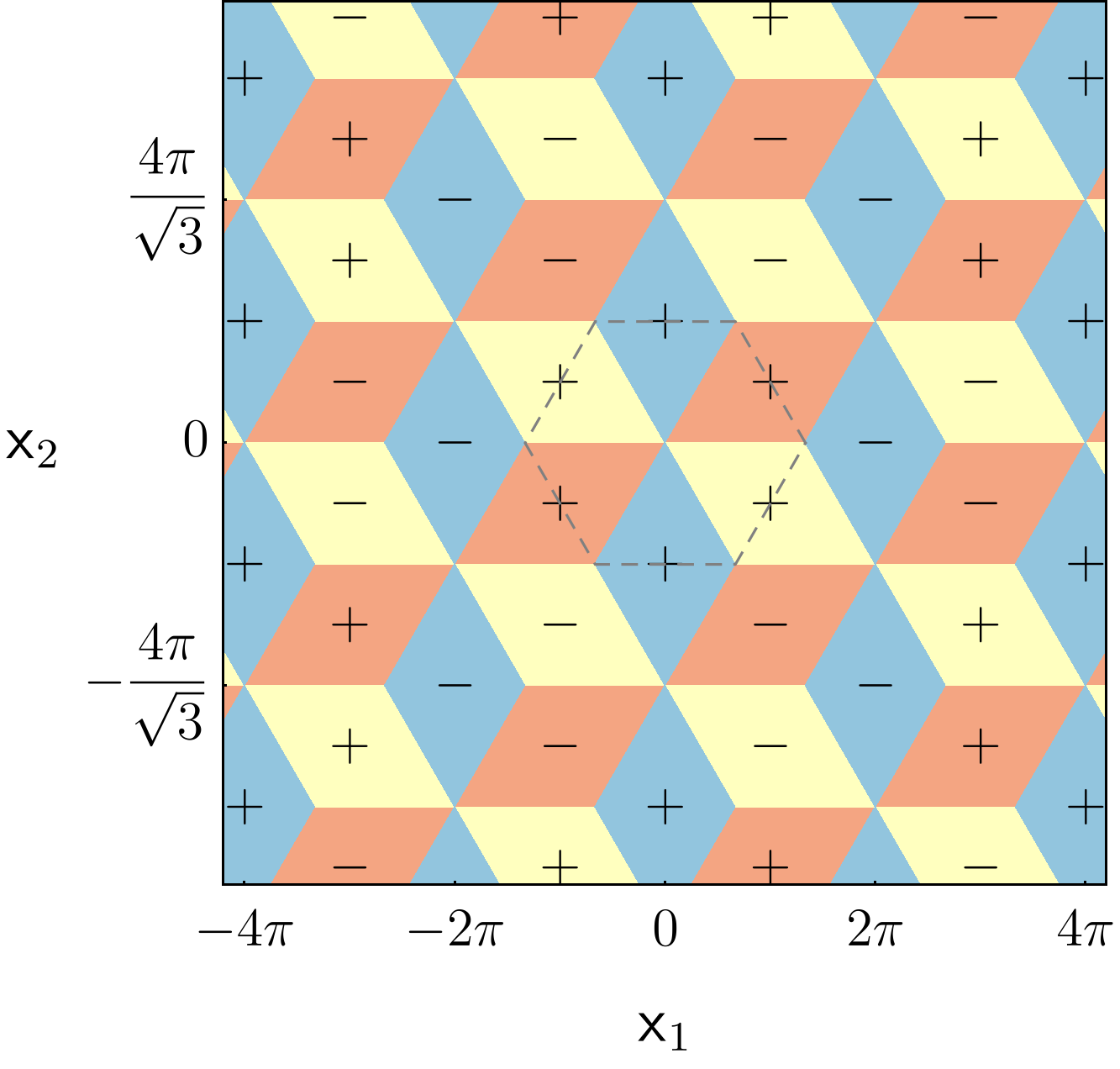
Having described the case of the Néel antiferromagnet in detail, we give further results more succinctly for other types of 2d magnets. The materials FePS3, CoPS3, and NiPS3 all have the same lattice structure as MnPS3 but exhibit “zig-zag” magnetic order. It is a collinear magnetic order which doubles the unit cell. There are three possible ordering wavevectors: the M points at the centers of the edges of the moiré Brillouin zone, which are half reciprocal lattice vectors, , with . The spin density (analogous to (5)) therefore contains three order parameter “flavors”, :
| (18) |
Here in a zig-zag state, just a single one of the three vectors is non-zero: this describes three possible spatial orientations of the zig-zag chains of aligned spins. Proceeding as before, we obtain the effective classical Hamiltonian in the form
| (19) | ||||
Here are two stiffness constants, and is a potential which may be taken in the form
| (20) |
with to model the energetic preference for a single non-zero stripe orientation, and as before to tune anisotropy.
(19) gives a continuum model to determine the magnetic ordering texture for arbitrary twist angles. The most important difference from the two-sublattice antiferromagnet is that here each spatial harmonic couples to a single “flavor”, while in the former case, (18), the single flavor of order parameter couples to the sum of harmonics. While we do not present a general solution, we note immediate consequences in the strong coupling limit, . In this situation, for each we must choose the largest harmonic, i.e. the which maximizes , and then take and for . Remarkably, the result is a tiling of six possible zig-zag domains which evokes a “dice lattice”, as shown in Fig. 3. Narrow domain walls separate these regions.
Twisted ferromagnet
Naïvely, twisting a homo-bilayer of ferromagnets is relatively innocuous. However, experiments and theory mcguire2015coupling; song2019switching; wang2018very; huang2018electrical; sivadas2018stacking; soriano2019interplay; jiang2019stacking for CrI3 have indicated that the interlayer exchange has a strength and sign that depends upon the displacement between neighboring layers. This can be directly incorporated into a continuum model following our methodology.
To this end, for a general twisted bilayer of a ferromagnetic material with the above property, one can use the energy functional shown in (8) with minimal modifications: i) the Néel vectors should be everywhere replaced by the uniform magnetization , since in fact each layer is ferromagnetic within itself and ii) the function takes a more complicated form. The latter may be determined from the dependence of the interlayer exchange of untwisted layers on a uniform interlayer displacement. For the case of CrI3, we have extracted the stacking dependent interlayer exchange data from the first principle calculations in Ref. sivadas2018stacking. Similar to the case of twisted antiferromagnets, a variational analysis of (8) can be performed, which leads to the same set of Euler-Lagrange equations, i.e. (12) and (13). In order to simplify the analysis, we will only consider an infinitesimal here; its effect is to fix the value of for CrI3 as discussed in the Supporting Information. The effects of non-zero can also be studied in a way similar to the previous case. The mathematical problem is then to obtain the functional form of and its dependence upon . In the ferromagnetic case, the Fourier expansion of generally has a nonzero constant term, which dominates the solution at small . In the case of CrI3, the constant term is small and ferromagnetic, thus is chosen for small . However, if other harmonics of are strong enough, a twisted solution starts to appear at a finite value of with a lower energy. As in the antiferromagnetic case, shows spatial modulations imitating the changes of in this twisted solution. This property of the twisted solution is most visible in the large limit, where the kinetic energy penalty is least important: one observes then domains with , separated by narrow domain walls. For a detailed analysis of the above statements in the case of CrI3, see the Supporting Information. A plot of the average magnetization in the system is shown in Fig. 4(a) with a transition form collinear to twisted phase at finite . Unlike the antiferromagnets discussed above, there is a finite interval of twist angles where the collinear phase exists even with infinitesimal anisotropy parameter . Also a plot of the spatial configuration of a twisted solution is presented in Fig. 4(b); it shows that there are large regions in real space with maximal magnetization while at the same time there are also other regions exhibiting zero magnetization.


Conclusion
In this work, we have considered moiré two dimensional magnets and in particular the twisted bilayers of Van der Waals magnetic materials. We have developed a low energy formalism in the continuum and studied in detail three different examples of twisted bilayers: antiferromagnetic, zig-zag antiferromagnetic and ferromagnetic. Remarkably, a rich phase diagram is obtained as one varies the twist angle and material parameters; there are interesting twisted ground state solutions comprising long-wavelength non-collinear magnetic textures. Such spatial patterns can potentially be observed in experiments, where the twist angle control adds to the tunability of the system. Furthermore, at small twist angles in the non-collinear phases, certain spin waves also exhibit interesting features such as flattening dispersion curves.
Material-wise, MnPS3 has , and the system is in the collinear phase for generic twist angles. The ratio was derived using and , where the intralayer exchange , interlayer coupling and the magnon gap are extracted from Wildes. On the other hand, for CrI3, we have derived using the intralayer exchange and anisotropy parameter as given in Ref. chen2018topological, and the interlayer exchange data as given in Ref. sivadas2018stacking. A plot of average magnetization for CrI3 in the perpendicular and parallel directions for which the above parameters are used is presented in Fig. 4(a) in the bottom panel; it can be seen that at large angles, the system is in the collinear phase, but the twisted-s phase () starts to be preferred at ; upon further decreasing the angle, starting at , the twisted-a phase becomes the ground state. This shows that in a twisted bilayer of CrI3, it is reasonable to expect both of the twisted phases to be realized in experimentally accessible settings.
The present methodology can be utilized with minimal modifications in further analyses of other moiré systems in the vast collection of possible bilayer magnetic materials. Their magnetic properties as well as their interplay with the electronic/transport properties could be the subject of future studies. Given the extremely fruitful research done in the field of moiré electronic systems, one can anticipate that the magnetic moiré systems could play the role of a new platform where novel exciting physics could be pursued.
We take some space in this section to explain our numerical manipulations.
- •
In order to find the ground states, one needs to solve (12) and (13) simultaneously. We have done so by two different methods: first solving the equations in real space by the use of overdamped dynamics, i.e. adding fictitious time derivatives of and to the equations and running the time evolution; a final configuration with zero time derivative ensures that the equations are satisfied. The second method is solving the equations in the Fourier representation iteratively by starting from a well-chosen simple guess; most of the time is a suitable initial seed. The results from the above two approaches agree completely.
- •
In figure 1, the phase boundaries can be extracted by observing the changes of behavior of and . We first solve the equations of motion (12) and (13) for various combinations of and , and plot the corresponding functions and in real space. In the collinear phase, both are constants. Fixing while increasing from zero, will begin to have spatial variation at the phase boundary between the collinear and the twisted-s phase. On the other hand, if one fixes while increasing from zero, the will start from a constant in the twisted-s phase and begin to have spatial variations once it crosses the phase boundary and enters the twisted-a phase.
- •
As for figure 2(c), the spin waves are obtained from the Bloch ansatz and similarly for . The variables in equations (17) thus become , with the substitutions and . Discretizing the Moiré unit cell, the linear operators become large matrices and can subsequently be diagonalized using Mathematica to find the magnon bands.
- •
The interlayer exchange for CrI3 is extracted from Fig. 2b of Ref. sivadas2018stacking, where the dependence upon displacement is presented along two special lines. The interlayer exchange is a periodic function with the same period as that of the monolayer lattice; thus, a Fourier series for the interlayer exchange (a constant along with the lowest five harmonics) in the two dimensional space is assumed which induces one dimensional functions on the above two special lines; one can fix the Fourier coefficients by comparing the given functional form and the one induced by the two dimensional Fourier series. The equations are solved using the same method described above.
All codes are available upon request.
We thank Andrea Young for useful discussions. This work was supported by the Simons Collaboration on Ultra-Quantum Matter, grant 651440 from the Simons Foundation (LB,ZL), and by the DOE, Office of Science, Basic Energy Sciences under Award No. DE-FG02-08ER46524 (KH).
References
- (1) KS Novoselov, A Mishchenko, A Carvalho, AH Castro Neto, 2d materials and van der waals heterostructures. \JournalTitleScience 353 (2016).
- (2) KS Burch, D Mandrus, JG Park, Magnetism in two-dimensional van der waals materials. \JournalTitleNature 563, 47–52 (2018).
- (3) ND Mermin, H Wagner, Absence of ferromagnetism or antiferromagnetism in one- or two-dimensional isotropic heisenberg models. \JournalTitlePhys. Rev. Lett. 17, 1133–1136 (1966).
- (4) L Savary, L Balents, Quantum spin liquids: a review. \JournalTitleReports on Progress in Physics 80, 016502 (2017).
- (5) G Ouvrard, R Brec, J Rouxel, Synthesis and physical characterization of the lamellar compound cops3. \JournalTitleChemischer Informationsdienst 13, no–no (1982).
- (6) G Le Flem, R Brec, G Ouvard, A Louisy, P Segransan, Magnetic interactions in the layer compounds mpx3 (m=mn, fe, ni; x=s, se). \JournalTitleJ. Phys. Chem. Solids 43, 455 (1982).
- (7) K Kurosawa, S Saito, Y Yamaguchi, Neutron diffraction study on mnps3 and feps3. \JournalTitleJ. Phys. Soc. Jpn. 52, 3919 (1983).
- (8) G Ouvrard, Ph.D. thesis (Nantes, France) (1980).
- (9) R Brec, Review on structural and chemical properties of transition metal phosphorous trisulfides mps3. \JournalTitleSolid State Ionics 22 (1986).
- (10) B Huang, et al., Layer-dependent ferromagnetism in a van der waals crystal down to the monolayer limit. \JournalTitleNature 546, 270–273 (2017).
- (11) R Bistritzer, AH MacDonald, Moiré bands in twisted double-layer graphene. \JournalTitleProceedings of the National Academy of Sciences 108, 12233–12237 (2011).
- (12) L Balents, General continuum model for twisted bilayer graphene and arbitrary smooth deformations. \JournalTitleSciPost Phys. 7, 48 (2019).
- (13) AR Wildes, B Roessli, B Lebech, KW Godfrey, Spin waves and the critical behaviour of the magnetization in mnps3. \JournalTitleJ. Phys.: Condens. Matter 10, 6417–6428 (1998).
- (14) MA McGuire, H Dixit, VR Cooper, BC Sales, Coupling of crystal structure and magnetism in the layered, ferromagnetic insulator cri3. \JournalTitleChemistry of Materials 27, 612–620 (2015).
- (15) T Song, et al., Switching 2d magnetic states via pressure tuning of layer stacking. \JournalTitleNature Materials 18, 1298–1302 (2019).
- (16) Z Wang, et al., Very large tunneling magnetoresistance in layered magnetic semiconductor cri 3. \JournalTitleNature communications 9, 2516 (2018).
- (17) B Huang, et al., Electrical control of 2d magnetism in bilayer cri 3. \JournalTitleNature nanotechnology 13, 544 (2018).
- (18) N Sivadas, S Okamoto, X Xu, CJ Fennie, D Xiao, Stacking-dependent magnetism in bilayer cri3. \JournalTitleNano letters 18, 7658–7664 (2018).
- (19) D Soriano, C Cardoso, J Fernández-Rossier, Interplay between interlayer exchange and stacking in cri3 bilayers. \JournalTitleSolid State Communications 299, 113662 (2019).
- (20) P Jiang, et al., Stacking tunable interlayer magnetism in bilayer cri 3. \JournalTitlePhysical Review B 99, 144401 (2019).
- (21) L Chen, et al., Topological spin excitations in honeycomb ferromagnet cri 3. \JournalTitlePhysical Review X 8, 041028 (2018).
Moiré magnets Kasra Hejazi, Zhu-Xi Luo and Leon Balents
Supporting Information Text
0.1 Linear wave analysis with anisotropy
In this section, we present the magnon spectrum when the anisotropy is present, and separately discuss the cases of Ising anisotropy () and XY anisotropy ().
Ising Anisotropy
Following the parametrization in equation (15), The Hamiltonian near the saddle point is
| (21) |
where the first line is the 0th order contribution, and the dots in the end represent higher-order terms in and . Switching to the symmetric and anti-symmetric basis, this becomes
| (22) |
where is defined in equation (10) of the main text.
For the second order terms of the Hamiltonian, we go to the Lagrangian by
| (23) |
which leads to the following coupled linear wave equations for ’s:
| (24) |
Taking and using the Bloch ansatz (with being the dimensionless quasi-momentum vector),
| (25) |
we obtain
| (26) |
In the collinear phase, the Neel vectors in the two layers are uniform and point either to the or the direction. Namely, there are four possible combinations that are degenerate in energy: and . The last two of them satisfying have the same discrete symmetry as that of the twisted-s phase, i.e. a simultaneous spin reflection and layer exchange. For this type of solutions, (26) reduces to a pair of degenerate equations for and :
| (27) |
For the other two solutions with , (26) reduces to a pair of degenerate equations for and instead. The and modes satisfy the same set of equations as in (27) upon substituting . We will choose the case below for concreteness.
The twisted-a phase is the only one that involves the interplay between the symmetric and anti-symmetric modes. As can be observed from (26), the modes are mixed, so are and ; the four branches thus combine into two, which we will simply label as and . There is one Goldstone mode in the -branch. In the twisted-s phase, the four equations decouple, and there is again one Goldstone mode corresponding to the out-of-plane rotation .
| (28) |
The magnon bands in the three phases are shown in figure S5.
Similar to the isotropic case, the magnon bands flatten at large due to their confinement in the disconnected domains in a large potential. Below we show an example in the twisted-a phase.
XY Anisotropy
Finally, we turn to the case , where the Neel vectors tend to lie in the XY plane. We thereby choose the following ansatz:
| (29) |
The Hamiltonian at the saddle point is . Classically, it behaves as if there is no anisotropy, and is uniform everywhere. Near the saddle point, following the same procedure as the section above, we obtain in the symmetric/anti-symmetric basis:
| (30) |
where the parametrization has been used in the last line, which is slightly modified from that in the main text. The corresponding Lagrangian then leads to the following linear wave equations:
| (31) |
All the four branches decouple and almost reduce to the the isotropic form as in the main text, up to the constant shift of in the -branches. Under the Bloch ansatz, the above equations become
| (32) |
There is one Goldstone mode in the branch, corresponding to the rotation in the XY plane. As increases, we will again observe the flattening of and bands. We plot an example in the twisted phase in the figure S7 below.
0.2 General perturbative solution of the Euler Lagrange equations
We will encounter the following energy functional and the subsequent partial differential equation in different situations in this work and thus we will first present a general study here. One needs to minimize an energy functional of the following form:
| (33) |
is a periodic function defining a triangular lattice, and it has zero mean over one unit cell. One can write a Fourier expansion for in terms of the reciprocal lattice vectors of the above traingular lattice:
| (34) |
We will be seeking solutions for that minimize the energy functional above and are periodic with the same period as that given by . There is always a trivial solution , with an average energy per unit cell equal to . Here we present a perturbative calculation of a nontrivial solution when and are small; these two parameters are taken to be small with their ratio kept a constant.
In order to find the function that minimizes the above energy functional, we will use the following Euler Lagrange equation:
| (35) |
which should be solved with periodic boundary conditions. Since, we are interested in the specific limit of both and being small, while keeping their ratio a constant, we will add a bookkeeping parameter to keep track of orders in our perturbation; we will ultimately set . The equation thus takes the form:
| (36) |
We will find a nontrivial solution as a power series in :
| (37) |
To zeroth order in , one needs to be a constant, this constant will be determined in higher orders:
| (38) |
To first order in , the differential equation takes the form:
| (39) |
It could be satisfied if takes the form:
| (40) |
where denotes a constant needed in the first order solution, this constant should also be fixed using higher orders of the equation. The second order in of the differential equation now reads:
| (41) |
The left hand side of the above equation does not contain a component while the right hand side does:
| (42) |
This needs to vanish so that the second order differential equation holds, and this fixes the value of :
| (43) |
This result shows that for values of smaller than , a nontrivial solution could exist. Furthermore, the second order part of could be found also using (41):
| (44) | ||||
with the constant determined again by higher orders of the differential equation.
This procedure can be carried out order by order, we will just state the result for , which could be derived from the component of the order of the differential equation:
| (45) |
Also, the average energy density per unit cell can be found to be:
| (46) |
where denotes any cubic power of and . This energy should be compared with the trivial solution energy density, i.e. ; the twisted solution, when it exists, has lower energy to this order and thus it is the true ground state for . At , interestingly, the two solutions coincide and thus this transition is continuous.
Finally we would like to emphasize that the above perturbative expansion works when both and are small with their ratio kept constant; could be small or order one but the perturbation breaks down for large . Below, we will elaborate on the three cases that the above perturbative calculation has been used in this work.
0.3 Twisted antiferromagnets
One should consider solving the following Euler-Lagrange equations for a twisted antiferromagnet as discussed in the main text:
| (47) | ||||
| (48) |
with and . One can find a nontrivial twisted solution (which we call twisted-s) in the main text, by setting or ; it will be shown below that the solution has lower energy. Starting from the twsited-s solution, increasing at small results in a transtion to the collinear phase, while on the other hand for large , with increasing , one encounters a transition to the twisted-a phase. We will discuss these two cases separately below.
Transtion from the twisted-s phase to the collinear phase, large angles
At large angles, both and are small and we will treat the Euler-Lagrange equations perturbatively. With choosing or , the equations read:
| (49) |
where corresponds to and corresponds to , and we will be considering the limit where the ratio is kept constant, so that we can use the perturbation series developed above; plays the role of , and plays the role of . The solution can be found order by order as discussed above:
| (50) |
The energy density can also be calculated which leads to:
| (51) |
This result is kept to one higher order than the previous section; it is this higher order which shows that is preferred energetically and so the sign should be chosen throughout.
Also, it is worthwhile to note that the limit of , corresponds to , which simply means that to lowest order in .
Transition from twisted-s phase to the twisted-a phase, small angles
At small angles, where is large but is kept still small, one can take the configuration of to be completely determined by satisfying the term in the Hamiltonian: can be taken equal to . This forms domains of constant , with narrow domain walls between them. On the other hand, should be found using the Euler-Lagrange equations, which reduce to:
| (52) |
For small , we can use the perturbation theory developed above, with , and (remember that is not dynamical in the above equation) playing the roles of , and respectively in (35). One can see that a twisted solution with exists, if is large enough. It is found numerically that
which means that domains with antiferromagnetic interlayer exchange have larger area than those with ferromagnetic interlayer coupling. Furthermore, one can also find numerically that
These two values show that a twisted solution for could appear if ; this should correpsond to the value for which the transition between twisted-s and twisted-a phases occurs at large , and it is indeed very close, with a few percent error actually, to the value found numerically at large in the phase diagram presented in the main text.
0.4 Twisted ferromagnetic CrI3 bilayer
For the properties of the interlayer exchange parameter in a bilayer CrI3 system, we will be following the numerical results presented in Ref. sivadas2018stacking, where first-principles calculations are carried out: it is shown that the interlayer exchange can vary considerably if the bilayer stacking is altered, and in fact it can change its sign; the pristine CrI3 bilayer exhibits antiferromagnetic interlayer exchange, but the above statement implies that this can be modified if the stacking is varied. Remarkably in a twisted bilayer, the displacement between the layers is modulated periodically with a unit cell given by the moiré length and so all the different kinds of displaced bilayer stacking are realized. With this in mind, one can use the energy functional discussed in the main text
| (53) |
where, as discussed in the main text, the function takes a form that should be extracted from the calculations of the stacking dependence of interlayer exchange as obtained for example in Ref. sivadas2018stacking.
We have used the plots presented in Ref. sivadas2018stacking, to find the Fourier components of the interlayer exchange which is indeed a periodic function of the interlayer displacement. It turns out that unlike the antiferromagnetic case initially studied in the main text, i.e. , the present function needs several harmonics along with a constant term to be reproduced (see Fig. S8). We will ultimately work with a rescaled Hamiltonian that has a form that is identical to that in the antiferromagnetic case:
| (54) |
and are defined as before and , where ’s are the rescaled moiré reciprocal lattice vectors. We have kept the lowest five harmonics along with the constant term here. Furthermore, is normalized in a way that Variation of this energy functional leads to the same set of equations
| (55) | ||||
| (56) |
which should be solved to minimize the energy here also. We will only discuss the case of a positive infinitesimal here, the case of general positive should be similar to the antiferromagnetic case. The effect of a positive infinitesimal is to fix a value for , and in this case it turns out that is energetically favored; this will be justified below.
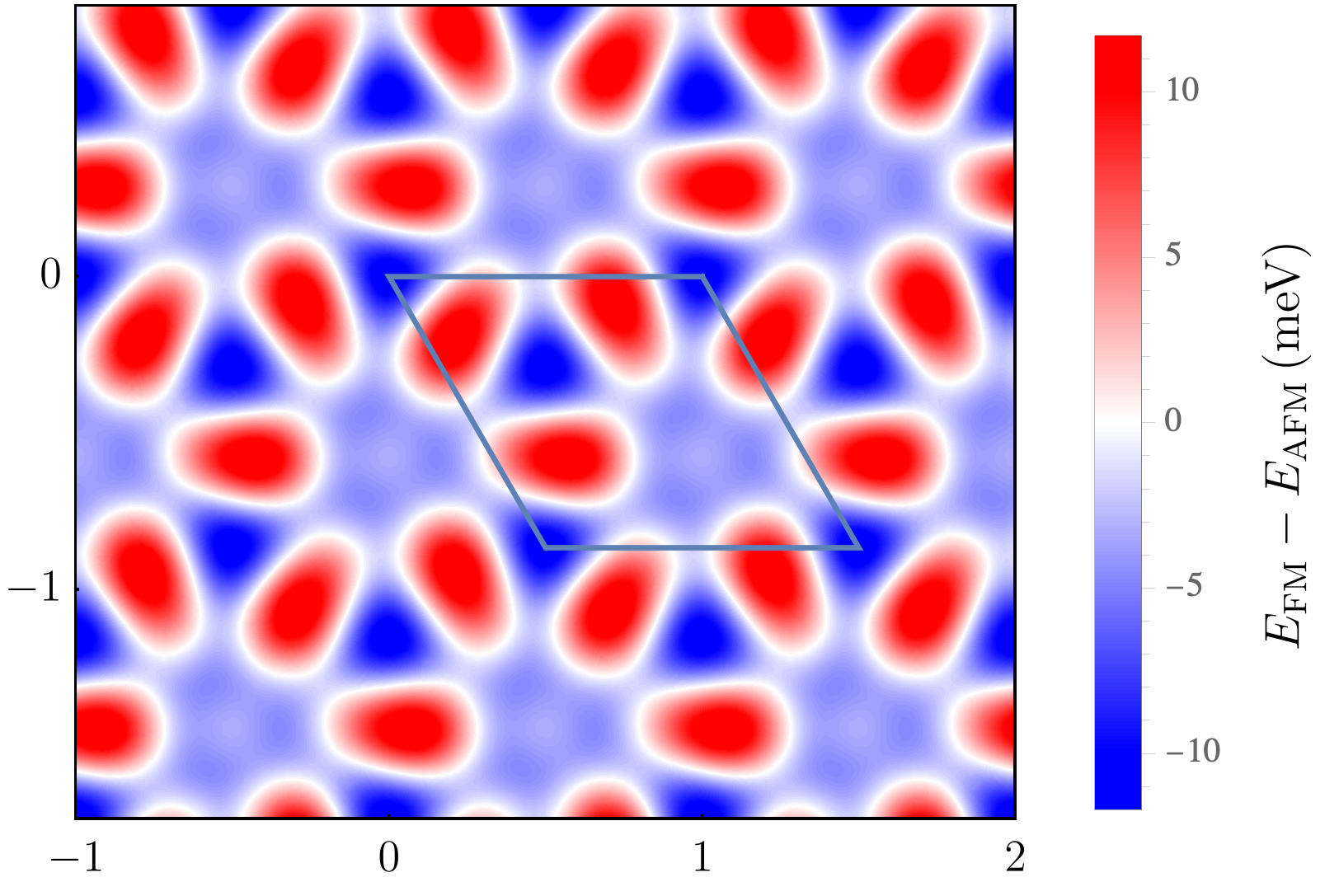
The only functionality that needs to be determined now is that of , and the only parameter is ; this time has a nonzero constant term as well, and thus at small the configuration is totally controlled by this constant term; we have derived which means that this constant imposes ferromagetic interlayer exchange, and thus the solution at small turns out to be , with an energy density . One expects this trivial state to give way to a twisted solution with lower energy at some value of ; since is small itself, the transition to a twisted phase happens at a small and thus one can set up a perturbative calculation for the twisted solution of at small ; this perburbative calculation, which is discussed in Sec. 0.2 of the SM, yields
| (57) |
with . This means that the twisted solution exists for above to leading order. The energy density for this state turns out to be to leading order; this shows that indeed a continuous transition to the twisted phase happens at .
For very large values of similar to what happens in the twisted antiferromagnets discussed in the main text, the twisted solution implies that is either or almost everywhere, so that except for narrow domain wall regions where .
Here we can see why is chosen for an infinitesimal positive in two different limits: at small , the constant term is ferromagnetic and thus the energy will decrease by setting ; for large on the other hand, since one is in the extreme twisted phase, one should note that the area with ferromagnetic interlayer coupling is larger than that with antiferromagnetic coupling, or in other words
and thus is again energetically favored. It is worthwhile to mention that this is a coincidence in CrI3, that both small and large limits prefer interlayer ferromagnetism; this could well not be the case in other materials in which cases it is reasonable to expect a transition at intermediate from to .
References
- (1) KS Novoselov, A Mishchenko, A Carvalho, AH Castro Neto, 2d materials and van der waals heterostructures. \JournalTitleScience 353 (2016).
- (2) KS Burch, D Mandrus, JG Park, Magnetism in two-dimensional van der waals materials. \JournalTitleNature 563, 47–52 (2018).
- (3) ND Mermin, H Wagner, Absence of ferromagnetism or antiferromagnetism in one- or two-dimensional isotropic heisenberg models. \JournalTitlePhys. Rev. Lett. 17, 1133–1136 (1966).
- (4) L Savary, L Balents, Quantum spin liquids: a review. \JournalTitleReports on Progress in Physics 80, 016502 (2017).
- (5) G Ouvrard, R Brec, J Rouxel, Synthesis and physical characterization of the lamellar compound cops3. \JournalTitleChemischer Informationsdienst 13, no–no (1982).
- (6) G Le Flem, R Brec, G Ouvard, A Louisy, P Segransan, Magnetic interactions in the layer compounds mpx3 (m=mn, fe, ni; x=s, se). \JournalTitleJ. Phys. Chem. Solids 43, 455 (1982).
- (7) K Kurosawa, S Saito, Y Yamaguchi, Neutron diffraction study on mnps3 and feps3. \JournalTitleJ. Phys. Soc. Jpn. 52, 3919 (1983).
- (8) G Ouvrard, Ph.D. thesis (Nantes, France) (1980).
- (9) R Brec, Review on structural and chemical properties of transition metal phosphorous trisulfides mps3. \JournalTitleSolid State Ionics 22 (1986).
- (10) B Huang, et al., Layer-dependent ferromagnetism in a van der waals crystal down to the monolayer limit. \JournalTitleNature 546, 270–273 (2017).
- (11) R Bistritzer, AH MacDonald, Moiré bands in twisted double-layer graphene. \JournalTitleProceedings of the National Academy of Sciences 108, 12233–12237 (2011).
- (12) L Balents, General continuum model for twisted bilayer graphene and arbitrary smooth deformations. \JournalTitleSciPost Phys. 7, 48 (2019).
- (13) AR Wildes, B Roessli, B Lebech, KW Godfrey, Spin waves and the critical behaviour of the magnetization in mnps3. \JournalTitleJ. Phys.: Condens. Matter 10, 6417–6428 (1998).
- (14) MA McGuire, H Dixit, VR Cooper, BC Sales, Coupling of crystal structure and magnetism in the layered, ferromagnetic insulator cri3. \JournalTitleChemistry of Materials 27, 612–620 (2015).
- (15) T Song, et al., Switching 2d magnetic states via pressure tuning of layer stacking. \JournalTitleNature Materials 18, 1298–1302 (2019).
- (16) Z Wang, et al., Very large tunneling magnetoresistance in layered magnetic semiconductor cri 3. \JournalTitleNature communications 9, 2516 (2018).
- (17) B Huang, et al., Electrical control of 2d magnetism in bilayer cri 3. \JournalTitleNature nanotechnology 13, 544 (2018).
- (18) N Sivadas, S Okamoto, X Xu, CJ Fennie, D Xiao, Stacking-dependent magnetism in bilayer cri3. \JournalTitleNano letters 18, 7658–7664 (2018).
- (19) D Soriano, C Cardoso, J Fernández-Rossier, Interplay between interlayer exchange and stacking in cri3 bilayers. \JournalTitleSolid State Communications 299, 113662 (2019).
- (20) P Jiang, et al., Stacking tunable interlayer magnetism in bilayer cri 3. \JournalTitlePhysical Review B 99, 144401 (2019).
- (21) L Chen, et al., Topological spin excitations in honeycomb ferromagnet cri 3. \JournalTitlePhysical Review X 8, 041028 (2018).