Rank-one Detector for Kronecker-Structured Constant Modulus Constellations

In this scheme, the basis constellation set $\Phi_{0}\in\left\{1,\quad e^{j\pi}\right\}$ is a BPSK constellation while the remaining $P-1$ constellation sets are binary-PSKs related by a fixed successive rotation of $\frac{\pi}{2^{p}}$, $p=1,\dots,P-1$, applied to the basis BPSK constellation in the clock wise direction as

For illustration purposes, let us consider the case of a $8$-PSK constellation shown in Fig. 1. There is a minimum of $P=\log_{2}(8)=3$ binary-PSK constellation sets required to generate the $8$-PSK one. The first constellation $\Phi_{0}$ is the well-known BPSK one, as shown in Fig. 1(a). The second and third ones, are special binary-PSK constellations $\Phi_{1}$ and $\Phi_{2}$ as shown in Fig. 1(b) and Fig. 1(c), respectively. Note that the Kronecker products involving the three constellations in Figs. 1(a)-1(c) result in a conventional $8$-PSK constellation, as shown in Fig. 1(d). Table I provides some examples of Kronecker-structured constellations designed for QPSK and 8-PSK.

In scheme 2, the basis constellation $\Phi_{0}$ is taken from any known $M_{p}\textrm{-PSK},p=0,\dots,P-1$ constellation and the remaining constellation sets $\Phi_{p},p=1,\dots,P-1$ are lower or equal orders $M_{p}$-PSK, $p=1,\dots,P-1$. As an example, a $8$-PSK can be formed as the basis constellation $\Phi_{0}\in\textrm{BPSK}$, $\Phi_{1}\in\textrm{QPSK}$ and $\Phi_{2}\in 8\textrm{-PSK}$. Table I provides examples of 8-PSK Kronecker-structured constellations using different combinations of constellation sets. As a specific case, we can also assume repeated values of $M_{p}\leq M$, $p=0\ldots P-1$, which means that two or more constellation sets follow the same modulation cardinality, which is at most $M$.

The bit error probability $\text{P}(\Phi_{p})$ for each $p$-th binary-PSK using scheme 1 is given as

where $d_{\text{min}}^{p}$ is the minimum Euclidean distance between two binary-PSK symbols of the $\Phi_{p}$ (2). The range of minimum Euclidean distance for scheme 1 is $d_{\text{min}}\in\left\{\sqrt{2},2\right\}$ as shown in Fig. 1. For scheme 1, the overall probability of error is dominated by that of the binary constellation set $\Phi_{1}$ which is the one having the minimum Euclidean distance among the $P-1$ binary constellation sets. This can be seen by inspecting Eq. (2) and also in the example in Fig. 1. While, in scheme 2, all the constellations $\Phi_{p},p=0,\dots,P-1$ involved in the Kronecker product (1) are known $M_{p}$-PSK, consequently the error probability is well known in the literature for every individual constellation set $\Phi_{p}\in M_{p}\text{-PSK}$ [9]. Hence, the overall probability of error is dominated by the $M_{p}$-PSK, $p=0,\dots,P-1$ having maximum cardinality.

We consider a single-input-single-output (SISO) communication system. The received vector ${\mbox{\boldmath$y$}}[k]\in\mathbb{C}^{L\times 1}$ is given by

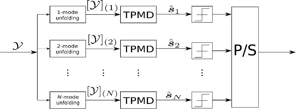
where ${\mbox{\boldmath$x$}}[k]\in\mathbb{C}^{L\times 1}$ is the transmitted data drawn from a constant modulus constellation, $h[k]$ represents the fading channel coefficient, $L$ is the length of the transmitted data block, and ${\mbox{\boldmath$n$}}[k]\sim\mathcal{C}\mathcal{N}({\mbox{\boldmath$0$}}_{L\times 1},\sigma_{n}^{2}{\mbox{\boldmath$I$}}_{L})$ is the additive white Gaussian noise, where $\sigma_{n}^{2}$ denotes its variance. The system model is shown in Fig. 2(a). Let us first give a high-level overview of the main blocks. At the transmitter, the serial bit stream is converted to $N$ parallel streams. At the $n$-th branch, the corresponding binary stream is modulated according to the available constellation sets $\Phi_{0},\dots,\Phi_{P-1}$, the design of which are detailed in the previous section for schemes 1 and 2. After the modulation, the Kronecker coding is applied and the resulting coded data block is transmitted. At the receiver, the Kronecker-RoD is applied to the received block, which is processed by multiple TPMD branches, as explained in $\mathrm{Section}$ III-B, to estimate the symbol vectors $\hat{{\mbox{\boldmath$s$}}}_{n}[k],n=1,\dots,N$, before demodulation and conversion back to a serial bit stream. We consider a Kronecker-structured constellation design for the transmitted data, which consists of “cross-coding” $N$ symbol vectors as follows

where ${\mbox{\boldmath$s$}}_{n}[k]\in\mathbb{C}^{L_{n}\times 1}$ , $n=\{1,\dots,N\}$, and $L=\Pi_{n=1}^{N}L_{n}.$ It is worth mentioning that the same constellation set $\Phi_{p}$, $\forall p=1,\ldots,P-1$, can be reused multiple times to map $\{{\mbox{\boldmath$s$}}_{n}[k]\},n=1,\dots,N$. Table II, provides some examples of constellation mappings for schemes 1 and 2, assuming $N\geq P$. The data rate in bits/symbol period (bit rate) is given as

Taking a closer look, we can conclude $\Upsilon_{\text{scheme 1}}\leq\Upsilon_{\text{scheme 2}}\leq\log_{2}M\Upsilon_{\text{scheme 1}}$, which shows that scheme 2 always has a higher data rate than scheme 1 by construction. In the special case with $M_{0}=M_{1},\dots=M_{P-1}=M$-PSK constellation, we have $\Upsilon_{\text{scheme 2}}=\log_{2}(M)\Upsilon_{\text{scheme 1}}$. Note that the data rates of both schemes are equal when BPSK is used to modulate the $N$ symbol vectors. In addition, assuming the same length for all the symbol vectors, say, $L_{n}=l$, the data rate boils down to $\frac{N\sum_{n=1}^{N}\log_{2}M_{n}}{l^{N}}$. Finally, the code rate R for the Kronecker-coding is given by $\frac{\sum_{n=1}^{N}L_{n}}{\Pi_{n=1}^{N}L_{n}}$.

The received signal after matched filtering is given by

For notational convenience, we skip the index $[k]$ in the rest of this paper, since it is irrelevant for the proposed detector. From (4) and (5), the estimation of the transmitted data $x$ can be translated into minimizing $\left\|\hat{{\mbox{\boldmath$y$}}}-{\mbox{\boldmath$s$}}_{N}\otimes\dots\otimes{\mbox{\boldmath$s$}}_{1}\right\|^{2}_{2}$ in the least squares sense. The key aspect is the fact that (5) can be recast as a rank-one $N$-th order tensor $\mathcal{X}={\mbox{\boldmath$s$}}_{1}\circ\dots\circ{\mbox{\boldmath$s$}}_{N}\in\mathbb{C}^{L_{1}\times L_{2}\times\dots\times L_{N}}$ so that the optimization problem can be reformulated as a tensor rank-one approximation problem

where $\hat{\mathcal{Y}}\in\mathbb{C}^{L_{1}\times L_{2}\times\dots\times L_{N}}$ is the $N$-th order “tensorized” received data tensor. Indeed, since $\mathcal{Y}$ is a scaled version of $\mathcal{X}$ corrupted by additive Gaussian noise, estimating the transmitted symbols ${\mbox{\boldmath$s$}}_{1},\dots,{\mbox{\boldmath$s$}}_{N}$ translates into finding a rank-one approximation to $\mathcal{Y}$. It is well known that a solution to this problem is provided by the truncated higher-order singular value decomposition (HOSVD)[10, 11]. An efficient way to compute this truncated rank-one HOSVD is the tensor power method [12, 13, 14]. As shown in [14], minimizing (8) is equivalent to maximizing the tensor Rayleigh quotient

For simplicity, let us define the following Gramian

where $n=1,\dots,N$. Note that the $n$-mode unfolding of the received tensor $\hat{\mathcal{Y}}$ can be expressed as

Assuming that the transmitted symbol vectors and noise are mutually uncorrelated, combining (10) and (11) yields

which shows that the $n$-th Gramian is a rank-one matrix corrupted by additive noise. We propose a tensor power method detector (TPMD) based on [12, 13, 14], where an estimate $\hat{{\mbox{\boldmath$s$}}}_{n},n=\{1,\dots,N\}$ is found from the dominant left singular vectors ${\mbox{\boldmath$u$}}_{n}\in\mathbb{C}^{L_{n}\times 1}$ (up to scaling) of the $n$-mode unfolding $\left[\mathcal{Y}\right]_{(n)}$ of the received data tensor $\mathcal{Y},n=1,\dots,N$. The TPMD starts from the initializations ${\mbox{\boldmath$u$}}_{1}^{(0)},\dots,{\mbox{\boldmath$u$}}_{N}^{(0)}$ of the $N$ symbol vectors, which are randomly drawn from the known alphabets that constitute the Kronecker-structured constellation, which are defined by the constellation sets $\Phi_{0},\ldots,\Phi_{P-1}$. At the $j$-th iteration, a new estimate is found by ${\mbox{\boldmath$u$}}_{n}^{(j)}={\mbox{\boldmath$A$}}_{n}{\mbox{\boldmath$u$}}_{n}^{(j-1)}$. Note that the number $N$ of TPMD branches corresponds to the $N$ symbols vectors ${\mbox{\boldmath$s$}}_{n}[k]$ that are Kronecker-coded using (5) as shown in Fig. 2(b). At the end of the $j$-th iteration, a normalized squared error is calculated as $e_{j}=\frac{\|{\mbox{\boldmath$u$}}_{n}^{(j)}-{\mbox{\boldmath$u$}}_{n}^{(j-1)}\|^{2}}{\|{\mbox{\boldmath$u$}}_{n}^{(j)}\|^{2}}$. The convergence is declared if $e_{j}\leq 10^{-6}$. The TPMD algorithm is summarized in Algorithm 1. On average, the TPMD takes less than 10 iterations for convergence, although our extensive simulations have shown that in the majority of the cases, the convergence is achieved within 3-4 iterations only. Due to the unknown norm of ${\mbox{\boldmath$u$}}_{n}$, we have $\hat{{\mbox{\boldmath$s$}}}_{n}=\beta_{n}{\mbox{\boldmath$s$}}_{n},n=\{n=1,\dots,N\}$, where $\beta_{n}$ is a scaling factor to be determined before demodulation. This factor can thus be calculated by using prior knowledge of the first element of ${\mbox{\boldmath$u$}}_{n}$ and ${\mbox{\boldmath$s$}}_{n}$ as $\beta_{n}=\frac{{\mbox{\boldmath$u$}}_{n}[1]}{{\mbox{\boldmath$s$}}_{n}[1]}$ (one single training symbol is enough for this purpose). The final estimate of the $n$-th symbol vector is then obtained as $\hat{{\mbox{\boldmath$s$}}}_{n}=\frac{{\mbox{\boldmath$u$}}_{n}}{\beta_{n}}$. Since the estimation of $\hat{{\mbox{\boldmath$s$}}}_{1},\dots,\hat{{\mbox{\boldmath$s$}}}_{N}$ can be carried out independently, the $N$ branches of the Kronecker-RoD shown in Fig. 2(b) can be executed in parallel. As far as the slicing procedure is concerned, once the convergence is achieved, the estimated symbols at the TPMD branches are projected onto their respective known alphabet sets $\Phi_{0},\dots,\Phi_{P-1}$. The complexity of the TPMD is that of executing a matrix-vector product in line 5 of Algorithm 1, which is given by $\mathcal{O}\left(8JL_{n}^{N}\right)$. The overall complexity of the Kronecker-RoD is $\mathcal{O}(8NJL_{n}^{N})$.

References

- [1] G. R. Patil and P. S.Wankhade, “5G wireless technology,” International Journal of Computer Science and Mobile Computing, vol. 3, no. 2, pp. 203–207, October 2014.
- [2] A. Goel and M. K. Garg, “Comparative performance evaluation of convolutionally coded and LDPC coded OFDM system over AWGN and SUI-5 fading channel,” in Proc. 2012 Third International Conference on Computer and Communication Technology, Nov 2012, pp. 250–254.
- [3] J. Porath and T. Aulin, “Design of multidimensional signal constellations,” IEE Proceedings - Communications, vol. 150, no. 5, pp. 317–, Oct 2003.
- [4] M. N. Khormuji, U. H. Rizvi, G. J. M. Janssen, and S. B. Slimane, “Rotation optimization for MPSK/MQAM signal constellations over Rayleigh fading channels,” in Proc. 2006 10th IEEE Singapore International Conference on Communication Systems, Oct 2006, pp. 1–5.
- [5] E. Biglieri, J. Proakis, and S. Shamai, “Fading channels: information-theoretic and communications aspects,” IEEE Transactions on Information Theory, vol. 44, no. 6, pp. 2619–2692, Oct 1998.
- [6] G. Hegde, Y. Yang, C. Steffens, and M. Pesavento, “Parallel low-complexity M-PSK detector for large-scale MIMO systems,” in Proc. 2016 IEEE Sensor Array and Multichannel Signal Processing Workshop (SAM), July 2016, pp. 1–5.
- [7] W. C. Freitas, G. Favier, A. L. F. de Almeida, and M. Haardt, “Two-Way MIMO Decode-and-Forward Relaying Systems with Tensor Space-Time Coding,” in Proc. 27th European Signal Processing Conference (EUSIPCO), Sep. 2019, pp. 1–5.
- [8] C. F. Van Loan and N. Pitsianis, “Approximation with Kronecker Products.” in Linear Algebra for Large Scale and Real-Time Applications, Springer, vol. 232, 1992, pp. 293–314.
- [9] Proakis, Digital Communications 5th Edition. McGraw Hill, 2007.
- [10] L. De Lathauwer, B. De Moor, and J. Vandewalle, “A multilinear singular value decomposition,” SIAM Journal on Matrix Analysis and Applications, vol. 21, no. 4, pp. 1253–1278, 2000.
- [11] T. G. Kolda and B. W. Bader, “Tensor decompositions and applications,” SIAM Review, vol. 51, no. 3, pp. 455–500, 2009.
- [12] L. De Lathauwer, P. Comon, B. D. Moor, and J. Vandewalle, “Higher-order power method - application in independent component analysis,” in Proc. NOLTA Conference, volume 1, pp. 91–96, Las Vegas,, 1995.
- [13] P. A. Regalia and E. Kofidis, “The higher-order power method revisited: convergence proofs and effective initialization,” in Proc. 2000 IEEE International Conference on Acoustics, Speech, and Signal Processing., vol. 5, June 2000, pp. 2709–2712 vol.5.
- [14] G. H. Golub and C. F. Van Loan, “Matrix Computations.” in 4th edition. Johns Hopkins University Press, Maryland, Baltimore, USA, 2013.
- [15] A. Graell i Amat, G. Montorsi, and S. Benedetto, “Design and decoding of optimal high-rate convolutional codes,” IEEE Transactions on Information Theory, vol. 50, no. 5, pp. 867–881, May 2004.
- [16] Y. Polyanskiy, H. V. Poor, and S. Verdu, “Channel coding rate in the finite blocklength regime,” IEEE Transactions on Information Theory, vol. 56, no. 5, pp. 2307–2359, May 2010.
- [17] G. Durisi, T. Koch, and P. Popovski, “Toward massive, ultrareliable, and low-latency wireless communication with short packets,” Proceedings of the IEEE, vol. 104, no. 9, pp. 1711–1726, Sep. 2016.
- [18] A. Viterbi, “Error bounds for convolutional codes and an asymptotically optimum decoding algorithm,” IEEE Transactions on Information Theory, vol. 13, no. 2, pp. 260–269, April 1967.
- [19] B. Moision, “A truncation depth rule of thumb for convolutional codes,” in Proc. 2008 Information Theory and Applications Workshop, Jan 2008, pp. 555–557.