跳到论文正文
W Papers独立论文阅读器 arXiv:2001.02707 论文正文 计算阅读时间 · 0%
引用这篇论文根据当前论文元数据生成,正式投稿前建议核对。


License: arXiv.org perpetual non-exclusive license
arXiv:2001.02707v2 [math.GT] 13 Mar 2020

Oriented Area as a Morse Function on Polygon SpacesThanks: The research is supported by «Native towns», a social investment program of PJSC «Gazprom Neft»

Daniil Mamaev Address: Chebyshev Laboratory, St. Petersburg State University, 14th Line V.O., 29, Saint Petersburg 199178 Russia Email address: dan.mamaev@gmail.com
Date: August 11, 2026(Last Typeset)
Abstract.

We study polygon spaces arising from planar configurations of necklaces with some of the beads fixed and some of the beads sliding freely. These spaces include configuration spaces of flexible polygons and some other natural polygon spaces. We characterise critical points of the oriented area function in geometric terms and give a formula for the Morse indices. Thus we obtain a generalisation of isoperimetric theorems for polygons in the plane.

2010 Mathematics Subject Classification
58K05, 52B60

1. Preliminaries: necklaces, configuration spaces, and oriented area function

Suppose one has a closed string with a number of labelled beads, a necklace. Some of the beads are fixed and some can slide freely (although the beads never pass through one another). Having the necklace in hand, one can try to put it on the plane (self-intersections are allowed) in such a way that the string is strained between every two consecutive beads. We will call this a (strained planar) configuration of the necklace. The space of all configurations (up to rotations and translations) of a given necklace, called configuration space of the necklace, together with the oriented area function on it is the main object of the present paper.

Let us now be precise. Given a tuple (n1,…,nk)(n_{1},\ldots,n_{k}) of positive integers and a tuple (L1,…,Lk)(L_{1},\ldots,L_{k}) of positive reals, we define a necklace 𝐍\mathbf{N} to be a tuple ((n1,L1),…,(nk,Lk))\big((n_{1},L_{1}),\ldots,(n_{k},L_{k})\big) interpreted as follows:

  • •

    the necklace has the total of n=n⁡(𝐍)=n1+…+nkn=n(\mathbf{N})=n_{1}+\ldots+n_{k} beads on it;

  • •

    kk of the beads are fixed and numbered by the index j=1,…,kj=1,\ldots,k in counter-clockwise order, the index jj is considered to be cyclic (that is, j=6​k+5j=6k+5 is the same as j=5j=5);

  • •

    there are (nj−1)(n_{j}-1) freely sliding beads between the jj-th and the (j+1)(j+1)-th fixed bead;

  • •

    the string has the total length of L=L⁡(𝐍)=L1+…+LkL=L(\mathbf{N})=L_{1}+\ldots+L_{k};

  • •

    the length of the string between the jj-th and the (j+1)(j+1)-th fixed bead is equal to LjL_{j}.

We fix the language we will talk about polygons in the present paper.

  • •

    A planar nn-gon is a collection of nn (labelled) points (p1,…,pn)(p_{1},\ldots,p_{n}) in the Euclidian plane ℝ2\mathbb{R}^{2}.

  • •

    The space of all planar nn-gons Polyn\mathop{\mathrm{Poly}}\nolimits_{n} is thus just (ℝ2)n\left(\mathbb{R}^{2}\right)^{n}.

  • •

    The sides of a polygon P=(p1,…,pn)P=(p_{1},\ldots,p_{n}) are the segments pi​pi+1p_{i}p_{i+1} for i=1,…,ni=1,\ldots,n, the length of the ii-th side is li=li​(P)=|pi​pi+1|l_{i}=l_{i}(P)=|p_{i}p_{i+1}|. Note that the index i=1,…,ni=1,\ldots,n is cyclic (that is, i=10​n+3i=10n+3 is the same as i=3i=3).

To avoid the messy indices, we introduce some additional notation associated with a necklace 𝐍=((n1,L1),…,(nk,Lk)){\mathbf{N}=\big((n_{1},L_{1}),\ldots,(n_{k},L_{k})\big)}. For index j=1,…,kj=1,\ldots,k

  • •

    we denote by j∗j^{*} the set of indices, corresponding to the jj-th piece of 𝐍\mathbf{N}:

    (1) j∗={n1+…+nj−1+1,…,n1+…+nj};j^{*}=\{n_{1}+\ldots+n_{j-1}+1,\ldots,n_{1}+\ldots+n_{j}\};
  • •

    we introduce a function ℒj:Polyn→ℝ\mathcal{L}_{j}\colon\mathop{\mathrm{Poly}}\nolimits_{n}\to\mathbb{R}, the total length of the sides of a polygon, corresponding to the jj-th piece of 𝐍\mathbf{N}, that is

    (2) ℒj​(P)=∑i∈j∗li​(P).\mathcal{L}_{j}(P)=\sum_{i\in j^{*}}l_{i}(P).

And now we are ready to give the following

Definition 1.1.

A (strained planar) configuration of necklace 𝐍=((n1,L1),…,(nk,Lk)){\mathbf{N}=\big((n_{1},L_{1}),\ldots,(n_{k},L_{k})\big)} is a polygon P∈PolynP\in\mathop{\mathrm{Poly}}\nolimits_{n} with ℒj​(P)=Lj\mathcal{L}_{j}(P)=L_{j} for all j=1,…,kj=1,\ldots,k.

Refer to caption
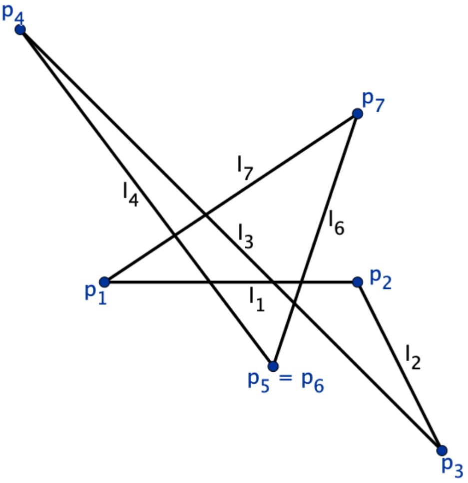
Figure 1. A polygon in ℳ⁡((2,l1+l2),(1,l3),(4,l4+l6+l7))\mathcal{M}\big((2,l_{1}+l_{2}),(1,l_{3}),(4,l_{4}+l_{6}+l_{7})\big)

All configurations of necklace 𝐍=((n1,L1),…,(nk,Lk))\mathbf{N}=\big((n_{1},L_{1}),\ldots,(n_{k},L_{k})\big) modulo translations and rotations form a space ℳ⁡(𝐍)=ℳ⁡((n1,L1),…,(nk,Lk))\mathcal{M}(\mathbf{N})=\mathcal{M}\big((n_{1},L_{1}),\ldots,(n_{k},L_{k})\big) called configuration space of necklace 𝐍\mathbf{N}. More formally,

  • •

    Consider all the strained planar configurations of 𝐍\mathbf{N}:

    (3) ℳ~(𝐍)=ℳ~((n1,L1),…,(nk,Lk))={P∈Polyn|ℒj​(P)=Lj​ for ​j=1,…,k}.\widetilde{\mathcal{M}}(\mathbf{N})=\widetilde{\mathcal{M}}\big((n_{1},L_{1}),\ldots,(n_{k},L_{k})\big)=\left\{P\in\mathop{\mathrm{Poly}}\nolimits_{n}\left|\begin{aligned} \mathcal{L}_{j}(P)=L_{j}\text{ for }j=1,\ldots,k\end{aligned}\right.\right\}.
  • •

    The group Isom+(ℝ2)\mathop{\mathrm{Isom}}\nolimits_{+}\left(\mathbb{R}^{2}\right) of orientation-preserving isometries of the Euclidean plane ℝ2\mathbb{R}^{2} acts diagonally on the space of all planar nn-gons Polyn=(ℝ2)n\mathop{\mathrm{Poly}}\nolimits_{n}=\left(\mathbb{R}^{2}\right)^{n}.

  • •

    ℳ~​(𝐍)\widetilde{\mathcal{M}}(\mathbf{N}) is invariant under the action.

  • •

    The configuration space of the necklace 𝐍\mathbf{N} is the space of orbits:

    (4) ℳ⁡(𝐍)=ℳ~​(𝐍)/Isom+(ℝ2).\mathcal{M}(\mathbf{N})=\left.\widetilde{\mathcal{M}}(\mathbf{N})\right/\mathop{\mathrm{Isom}}\nolimits_{+}(\mathbb{R}^{2}).
Definition 1.2.

Oriented area 𝒜\mathcal{A} of an nn-gon P=((x1,y1),…,(xn,yn))∈(ℝ2)n{P=((x_{1},y_{1}),\ldots,(x_{n},y_{n}))\in\left(\mathbb{R}^{2}\right)^{n}} is defined by

(5) 𝒜⁡(P)=12​|x1x2y1y2|+12​|x2x3y2y3|+…+12​|xnx1yny1|.\mathcal{A}(P)=\frac{1}{2}\begin{vmatrix}x_{1}&x_{2}\\ y_{1}&y_{2}\end{vmatrix}+\frac{1}{2}\begin{vmatrix}x_{2}&x_{3}\\ y_{2}&y_{3}\end{vmatrix}+\ldots+\frac{1}{2}\begin{vmatrix}x_{n}&x_{1}\\ y_{n}&y_{1}\end{vmatrix}.

Oriented area is preserved by the action of Isom+(ℝ2)\mathop{\mathrm{Isom}}\nolimits_{+}(\mathbb{R}^{2}) and thus gives rise to a well defined continuous function on (ℝ2)n/Isom+(ℝ2)\left(\mathbb{R}^{2}\right)^{n}/\mathop{\mathrm{Isom}}\nolimits_{+}(\mathbb{R}^{2}) hence on all of ℳ⁡(𝐍)\mathcal{M}(\mathbf{N}). We will denote these functions by the same letter 𝒜\mathcal{A}. The study of critical points (i. e. the solutions of d​𝒜​(P)=0d\mathcal{A}(P)=0) of 𝒜:ℳ⁡(𝐍)→ℝ\mathcal{A}\colon\mathcal{M}(\mathbf{N})\to\mathbb{R} is the substance of the present paper.

The paper is organised as follows. In Section 2 we review previously studied extreme cases: polygonal linkages (the ‘all beads are fixed’ case) and polygons with fixed perimeter (the ‘one bead is fixed’ case, which is clearly the same as ‘none of the beads are fixed’ case). In Section 3 we discuss the regularity properties of configuration spaces of necklaces. In the subsequent sections we study only non-singular part of configuration space. In Section 4 we give a geometric description of critical points of oriented area in the general case (Theorem 4.1) and deduce a formula for their Morse indices (Theorem 4.4) from Lemmata 4.5, 4.6, 4.7. In Section 5 the auxiliary Lemmata 4.5 and 4.6 concerning orthogonality of certain spaces with respect to the Hessian form of the oriented area function are proven. In Section 6 we discuss the ‘two consecutive beads are fixed’ case and give a proof of Lemma 4.7.

Acknowledgement

This research is a continuation of my bachelor thesis in which the case of configuration spaces of necklaces with two consecutive fixed beads was studied. I am deeply indebted to Gaiane Panina for posing the problem and supervising my research. I am also thankful to Joseph Gordon and Alena Zhukova for fruitful discussions and to Nathan Blacher for his valuable comments on the linguistic quality of the paper.

2. An overview of existing results

2.1. Configuration spaces of polygonal linkages

In the notation of the present paper these are the spaces ℳ⁡((1,l1),…,(1,ln)){\mathcal{M}((1,l_{1}),\ldots,(1,l_{n}))}, i. e. the spaces ℳ⁡(𝐍)\mathcal{M}(\mathbf{N}) for necklaces 𝐍\mathbf{N} with all beads being fixed. These spaces are studied in many aspects (see e. g. [2] or [3] for a thorough survey). On the side of studying oriented area on these spaces, the first general fact about its critical points was noticed by Thomas Banchoff (unpublished), reproved by Khimshiashvili and Panina [6] (their technique required some non-degeneracy assumptions) and then reproved again by Leger [9] in full generality.

Theorem 2.1 (Critical configurations in the ‘all beads are fixed’ case)
(Bunchoff, Khimshiashvili, Leger, and Panina).


Let 𝐍\mathbf{N} be a necklace with all the beads fixed. Then a polygon P∈ℳs​m​(𝐍){P\in\mathcal{M}_{sm}(\mathbf{N})} is a critical point of 𝒜\mathcal{A} if and only if it is cyclic (i. e. inscribed in a circle).

After describing critical points, the following natural question arises: are these critical points Morse (i. e. whether HessP𝒜\mathop{\mathrm{Hess}}\nolimits_{P}\mathcal{A}, the Hessian of 𝒜\mathcal{A} at PP, is a non-degenerate bilinear form on TP​ℳ​(𝐍)T_{P}\mathcal{M}(\mathbf{N})) and if they are, what is the Morse index (the dimension of maximal subspace on which HessP𝒜\mathop{\mathrm{Hess}}\nolimits_{P}\mathcal{A} is negative definite). The state-of-art answer to this question for the case of polygonal linkages requires some more definitions.

Definition 2.2.

Let PP be a cyclic polygon, oo the center of its circumscribed circle, and i∈{1,…,n}{i\in\{1,\ldots,n\}}.

  • •

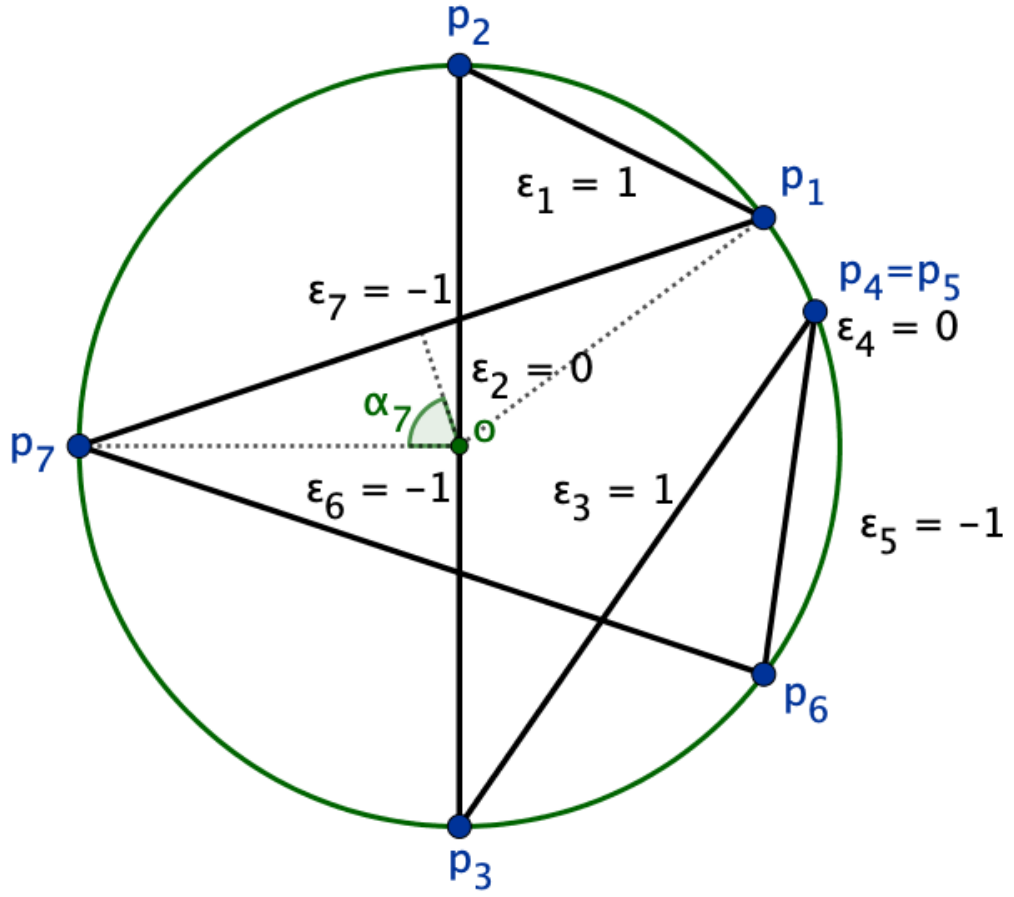
    the central half-angle of the ii-th side of PP is

    (6) αi​(P)=|∠​pi​o​pi+1|2∈[0,π/2]\alpha_{i}(P)=\frac{|\angle p_{i}op_{i+1}|}{2}\in[0,\pi/2]
  • •

    the orientation of the ii-th side of PP is

    (7) εi(P)={1, if ​∠​pi​o​pi+1∈(0,π);0, if ​∠​pi​o​pi+1∈{0,π};−1, if ​∠​pi​o​pi+1∈(−π,0).\varepsilon_{i}(P)=\left\{\begin{aligned} 1,\text{ if }\angle p_{i}op_{i+1}&\in(0,\pi);\\ 0,\text{ if }\angle p_{i}op_{i+1}&\in\{0,\pi\};\\ -1,\text{ if }\angle p_{i}op_{i+1}&\in(-\pi,0).\end{aligned}\right.
Refer to caption
Figure 2. A cyclic polygon with some notation

’ We will denote by 𝒞n\mathcal{C}_{n} the configuration space of cyclic polygons, more precisely,

(8) 𝒞n={P∈(ℝ2)n|P​ is a cyclic polygon;AffineHull(P)=ℝ2}/Isom+(ℝ2),\mathcal{C}_{n}=\left.\left\{P\in\left(\mathbb{R}^{2}\right)^{n}\left|\begin{aligned} P\text{ is a cyclic polygon};\\ \mathop{\mathrm{AffineHull}}\nolimits(P)=\mathbb{R}^{2}\end{aligned}\right.\right\}\right/\mathop{\mathrm{Isom}}\nolimits_{+}(\mathbb{R}^{2}),

For P∈𝒞nP\in\mathcal{C}_{n} we will denote by ΩP\Omega_{P} its circumscribed circle, by oPo_{P} the centre of ΩP\Omega_{P}, and by RPR_{P} the radius of ΩP\Omega_{P}.

Definition 2.3.

Let PP be a cyclic polygon with at least three different vertices. It is called admissible if no edge of PP passes through the center of its circumscribed circle. In this case its winding number wP=w⁡(P,o)w_{P}=w(P,o) with respect to the centre of circumscribed circle is well-defined.

Theorem 2.4 (Morse indices in the ‘all beads are fixed’ case)
(Gordon, Khimshiashvili, Panina, Teplitskaya, and Zhukova).


Let 𝐍\mathbf{N} be a necklace without freely moving beads, and let P∈ℳs​m​(𝐍){P\in\mathcal{M}_{sm}(\mathbf{N})} be an admissible cyclic polygon. Then PP is a Morse point of 𝒜\mathcal{A} if and only if ∑i=1nεitanαi≠0\sum\limits_{i=1}^{n}\varepsilon_{i}\tan\alpha_{i}\neq 0 and in this case its Morse index is

μP(𝒜)=#{i∈{1,…,n}:εi>0}−1−2wP−{0, if ∑i=1nεitanαi>0;1, otherwise.\mu_{P}(\mathcal{A})=\#\{i\in\{1,\ldots,n\}\colon\varepsilon_{i}>0\}-1-2w_{P}-\left\{\begin{aligned} 0,&\text{ if }\sum_{i=1}^{n}\varepsilon_{i}\tan\alpha_{i}>0;\\ 1,&\text{ otherwise}.\end{aligned}\right.

The formula more or less explicitly appeared in [7], [10], and [11], but in this form, with the precise condition of being Morse, the theorem was proved only in [4]. In view of the theorem, following [4], we give the following

Definition 2.5.

An admissible cyclic polygon PP is called bifurcating if ∑i=1nεitanαi=0\sum\limits_{i=1}^{n}\varepsilon_{i}\tan\alpha_{i}=0.

2.2. Configuration space of nn-gons with fixed perimeter

. This is the space ℳ⁡((,,,))\mathcal{M}((n,L)) (they are obviously the same for different LL so usually LL is set to 11). It is no secret since antiquity that the polygon in ℳ⁡((,,,))\mathcal{M}((n,L)) maximising oriented area is the convex regular one. But all the critical points of oriented area together with their indices were determined only in the recent paper [8] by Khimshiashvili, Panina and Siersma. Again, before stating the result, we give

Definition 2.6.

A regular star is a cyclic polygon PP such that all its sides are equal and have the same orientation (see (7)).

A complete fold is a regular star PP with pi=pi+2p_{i}=p_{i+2} for all i=1,…,ni=1,\ldots,n. It exists for even nn only.

Theorem 2.7 (Critical configurations and Morse indices in the ‘one bead is fixed’ case)
(Khimshiashvili, Panina, and Siersma).

  1. (1)

    ℳ⁡((,,,))\mathcal{M}((n,L)) is homeomorphic to ℂ​Pn−2\mathbb{C}\mathrm{P}^{n-2}.

  2. (2)

    A polygon P∈ℳs​m​((,,,))P\in\mathcal{M}_{sm}((n,L)) is a critical point of 𝒜\mathcal{A}, if and only if it is a regular star.

  3. (3)

    The stars with maximal winding numbers are Morse critical points of 𝒜\mathcal{A}.

  4. (4)

    Under assumption that all regular stars are Morse critical points, the Morse indices are:

    μP(𝒜)={2​wP−2, if wP<0;2​n−2​wP−2, if wP>0;n−2, if P​ is a complete fold.\mu_{P}(\mathcal{A})=\left\{\begin{aligned} &2w_{P}-2,&\text{ if }&w_{P}<0;\\ &2n-2w_{P}-2,&\text{ if }&w_{P}>0;\\ &n-2,&\text{ if }&P\text{ is a complete fold}.\end{aligned}\right.

They also prove a particularly insightful [8, Lemma 2]:

Lemma 2.8.

Let PP be a regular star which is not a complete fold with wP>0w_{P}>0. Then PP is a non-degenerate local maximum on 𝒞n\mathcal{C}_{n}.

In fact, this lemma together with Theorem 2.4 and Lemma 4.5 is enough to omit the assumptions in (4) of Theorem 2.7.

3. Singular locus of the configuration space

Definition 3.1.

Let PP be a configuration of necklace 𝐍=((n1,L1),…,(nk,Lk))\mathbf{N}=\big((n_{1},L_{1}),\ldots,(n_{k},L_{k})\big). It is called non-singular if ℒ=(ℒ1,…,ℒk)\mathcal{L}=(\mathcal{L}_{1},\ldots,\mathcal{L}_{k}) is a smooth submersion at PP (i. e. ℒ\mathcal{L} is differentiable at PP and its differential DPℒ:TPPolyn→TPℝkD_{P}\mathcal{L}\colon T_{P}\mathop{\mathrm{Poly}}\nolimits_{n}\to T_{P}\mathbb{R}^{k} is a surjective linear map), otherwise it is called singular.

First we give a geometric characterisation of singular configurations. Consider a polygon P=(p1,…,pn){P=(p_{1},\ldots,p_{n})}, with pi=(xi,yi)∈ℝ2p_{i}=(x_{i},y_{i})\in\mathbb{R}^{2} and li=|pi+1−pi|≠0l_{i}=|p_{i+1}-p_{i}|\neq 0 for all i=1,…,ni=1,\ldots,n and define βi\beta_{i} to be the oriented angle between vectors (1,0)(1,0) and (pi+1−pi){(p_{i+1}-p_{i})}. We also denote by s⁡(j)=n1+…+nj−1+1s(j)=n_{1}+\ldots+n_{j-1}+1 the index of the jj-th fixed bead. Then ℒj\mathcal{L}_{j} are differentiable at PP and the derivatives of ℒj\mathcal{L}_{j} with respect to xix_{i} and yiy_{i} look as follows:

(9) ∂ℒj∂xi​(P)\displaystyle\frac{\partial\mathcal{L}_{j}}{\partial x_{i}}(P) ={−cos⁡βi,ifi=s⁡(j);cos⁡βi−1−cos⁡βi,ifi∈j∗∖{s⁡(j)};cos⁡βi−1,ifi=s⁡(j+1);0,otherwise.\displaystyle=\left\{\begin{aligned} &-\cos\beta_{i},&\text{if}\;\,&i=s(j);\\ &\cos\beta_{i-1}-\cos\beta_{i},&\text{if}\;\,&i\in j^{*}\setminus\{s(j)\};\\ &\cos\beta_{i-1},&\text{if}\;\,&i=s(j+1);\\ &0,&\text{otherwise.}&\end{aligned}\right.
(10) ∂ℒj∂yi​(P)\displaystyle\frac{\partial\mathcal{L}_{j}}{\partial y_{i}}(P) ={−sin⁡βi,ifi=s⁡(j);sin⁡βi−1−sin⁡βi,ifi∈j∗∖{s⁡(j)};sin⁡βi−1,ifi=s⁡(j+1);0,otherwise.\displaystyle=\left\{\begin{aligned} &-\sin\beta_{i},&\text{if}\;\,&i=s(j);\\ &\sin\beta_{i-1}-\sin\beta_{i},&\text{if}\;\,&i\in j^{*}\setminus\{s(j)\};\\ &\sin\beta_{i-1},&\text{if}\;\,&i=s(j+1);\\ &0,&\text{otherwise.}&\end{aligned}\right.

The indices of the form s⁡(j)s(j) for j=1,…,kj=1,\ldots,k will be called boundary and all other indices will be called inner. We now establish a criterion for a configuration of a necklace to be singular.

Lemma 3.2.

A configuration P∈PolynP\in\mathop{\mathrm{Poly}}\nolimits_{n} of the necklace 𝐍=((n1,L1),…,(nk,Lk))\mathbf{N}=\big((n_{1},L_{1}),\ldots,(n_{k},L_{k})\big) is singular if and only if one of the following holds:

  1. (1)

    li=0l_{i}=0 for some i=1,…,ni=1,\ldots,n;

  2. (2)

    PP fits in a straight line in such a way that βi=βi−1\beta_{i}=\beta_{i-1} for all inner indices ii.

Proof.

The first condition is equivalent to ℒ\mathcal{L} being differentiable at PP. Therefore, what is left to prove, is that for P∈ℳ~​(𝐍)P\in\widetilde{\mathcal{M}}(\mathbf{N}) with no vanishing sides, the second condition hold if and only if the gradients gradPℒ1,…,gradPℒk\mathop{\mathrm{grad}}\nolimits_{P}\mathcal{L}_{1},\ldots,\mathop{\mathrm{grad}}\nolimits_{P}\mathcal{L}_{k} are linearly dependent.

Suppose that λ1​gradPℒ1+…+λk​gradPℒk=0\lambda_{1}\mathop{\mathrm{grad}}\nolimits_{P}\mathcal{L}_{1}+\ldots+\lambda_{k}\mathop{\mathrm{grad}}\nolimits_{P}\mathcal{L}_{k}=0 is a non-trivial vanishing linear combination. If λj≠0\lambda_{j}\neq 0, then, using formulae (9) and (10) for boundary index s⁡(j)s(j), we get −λjcosβs⁡(j)+λj−1cosβs⁡(j)−1=0-\lambda_{j}\cos\beta_{s(j)}+\lambda_{j-1}\cos\beta_{s(j)-1}=0 and −λjsinβs⁡(j)+λj−1sinβs⁡(j)−1=0-\lambda_{j}\sin\beta_{s(j)}+\lambda_{j-1}\sin\beta_{s(j)-1}=0. It means that points λj​(cos⁡βs⁡(j),sin⁡βs⁡(j))≠(0,0)\lambda_{j}(\cos\beta_{s(j)},\sin\beta_{s(j)})\neq(0,0) and λj−1​(cos⁡βs⁡(j)−1,sin⁡βs⁡(j)−1)\lambda_{j-1}(\cos\beta_{s(j)-1},\sin\beta_{s(j)-1}) coincide, which implies that 2​(βs⁡(j)−βs⁡(j)−1)=02(\beta_{s(j)}-\beta_{s(j)-1})=0 and λj−1=cos⁡(βs⁡(j)−βs⁡(j)−1)​λj≠0{\lambda_{j-1}=\cos(\beta_{s(j)}-\beta_{s(j)-1})\lambda_{j}}\neq 0. It follows then that λj≠0\lambda_{j}\neq 0 for all j=1,…,kj=1,\ldots,k, consequently, (we now use (9) and (10) for inner indices) βi=βi−1\beta_{i}=\beta_{i-1} for all inner indices ii, meaning that PP is composed of straight segments of lengths L1,…,LkL_{1},\ldots,L_{k}. Taking in account previously deduced formula 2​(βi−βi−1)=02(\beta_{i}-\beta_{i-1})=0 for boundary ii, we get that PP does satisfies condition (2). Reversing the above argument, we get the reverse implication. ∎

Now let ℳs​m~​(𝐍)\widetilde{\mathcal{M}_{sm}}(\mathbf{N}) be the set of non-singular configurations of necklace 𝐍\mathbf{N} and ℳs​m​(𝐍)\mathcal{M}_{sm}(\mathbf{N}) be the non-singular part of ℳ⁡(𝐍)\mathcal{M}(\mathbf{N}):

(11) ℳs​m(𝐍)=ℳs​m~​(𝐍)Isom+(ℝ2)={P∈Polyn|P​ is a non-singularconfiguration of ​𝐍}/Isom+(ℝ2)\mathcal{M}_{sm}\big(\mathbf{N})=\frac{\widetilde{\mathcal{M}_{sm}}(\mathbf{N})}{\mathop{\mathrm{Isom}}\nolimits_{+}(\mathbb{R}^{2})}=\left.\left\{P\in\mathop{\mathrm{Poly}}\nolimits_{n}\left|\begin{aligned} P\text{ is a non-singular}\\ \text{configuration of }\mathbf{N}\end{aligned}\right.\right\}\right/\mathop{\mathrm{Isom}}\nolimits_{+}(\mathbb{R}^{2})

If these spaces are non-empty, they are smooth manifolds, which generalises previous results on smoothness of configuration spaces of polygonal linkages by Kapovich—Millson [5] and Farber [3]. To state the precise result, we need the following

Definition 3.3.

A necklace 𝐍=((n1,L1),…,(nk,Lk))\mathbf{N}=((n_{1},L_{1}),\ldots,(n_{k},L_{k})\big) is called realisable if for all j=1,…,kj=1,\ldots,k, such that nj=1n_{j}=1, inequality 2​Lj<L1+…+Lk2L_{j}<L_{1}+\ldots+L_{k} holds.

Proposition 3.4.

Let 𝐍\mathbf{N} be a realisable necklace. Then

  1. (1)

    ℳs​m~​(𝐍)\widetilde{\mathcal{M}_{sm}}(\mathbf{N}) is a smooth submanifold of dimension 2​n−k2n-k in Polyn=ℝ2​n\mathop{\mathrm{Poly}}\nolimits_{n}=\mathbb{R}^{2n};

  2. (2)

    ℳs​m​(𝐍)\mathcal{M}_{sm}(\mathbf{N}) is a topological manifold of dimension 2​n−k−32n-k-3 with a unique smooth structure making the quotient map ℳs​m~​(𝐍)→ℳs​m​(𝐍)\widetilde{\mathcal{M}_{sm}}(\mathbf{N})\to\mathcal{M}_{sm}(\mathbf{N}) a smooth submersion;

  3. (3)

    the oriented area function 𝒜\mathcal{A} is a smooth function on ℳs​m​(𝐍)\mathcal{M}_{sm}(\mathbf{N}).

Proof.

It follows from Lemma 3.2, that the inequalities 2​Lj<L1+…+Lk2L_{j}<L_{1}+\ldots+L_{k} are necessary and sufficient for ℳs​m~​(𝐍)\widetilde{\mathcal{M}_{sm}}(\mathbf{N}) to be non-empty.

The first claim is clear since ℳs​m~​(𝐍)\widetilde{\mathcal{M}_{sm}}(\mathbf{N}) is locally a level of a smooth submersion ℒ=(ℒ1,…,ℒk):(ℝ2)n→ℝk{\mathcal{L}=(\mathcal{L}_{1},\ldots,\mathcal{L}_{k})\colon\left(\mathbb{R}^{2}\right)^{n}\to\mathbb{R}^{k}}.

To establish the second claim, we first note that ℳs​m​(𝐍)\mathcal{M}_{sm}(\mathbf{N}) is an orbit space of the action of 3-dimensional Lie group Isom+(ℝ2)\mathop{\mathrm{Isom}}\nolimits_{+}(\mathbb{R}^{2}) on smooth manifold ℳs​m~​(𝐍)\widetilde{\mathcal{M}_{sm}}(\mathbf{N}). Thus, it suffices to observe that the action is free and proper, which is indeed the case.

The third claim is obvious since the smooth structure on ℳs​m​(𝐍)\mathcal{M}_{sm}(\mathbf{N}) is induced from Polyn\mathop{\mathrm{Poly}}\nolimits_{n} and oriented area 𝒜\mathcal{A} (see Definition 1.2) is a smooth function on Polyn\mathop{\mathrm{Poly}}\nolimits_{n} preserved by the action of Isom+(ℝ2)\mathop{\mathrm{Isom}}\nolimits_{+}(\mathbb{R}^{2}). ∎

4. Main results: critical configurations and their Morse indices
in the general case

The first theorem describes critical points of oriented area on configuration spaces of necklaces, generalising Theorem 2.1 and (2) in Theorem 2.7. Recall that j∗j^{*} is the set of indices corresponding to the jj-th piece of a necklace (Definition 1) and εi​(P)\varepsilon_{i}(P) is an orientation of the ii-th side of a cyclic polygon PP (Definition 7).

Theorem 4.1 (Critical configurations in the general case).


A polygon P∈ℳs​m​((n1,L1),…,(nk,Lk))P\in\mathcal{M}_{sm}\big((n_{1},L_{1}),\ldots,(n_{k},L_{k})\big) is a critical point of 𝒜\mathcal{A} if and only if all of the following conditions hold:

  1. (1)

    PP is cyclic;

  2. (2)

    ∀i∈j∗:li​(P)=Lj/nj\forall i\in j^{*}\colon l_{i}(P)=L_{j}/n_{j};

  3. (3)

    ∀i1,i2∈j∗:εi1​(P)=εi2​(P)\forall i_{1},i_{2}\in j^{*}\colon\varepsilon_{i_{1}}(P)=\varepsilon_{i_{2}}(P).

Before proving the theorem, let us make two remarks.

Remark 4.2.

The statement of the theorem in plane English goes as follow: a non-singular configuration of a necklace is a critical point of oriented area if and only if all the beads lie on some circle in such a way that the arc between every two consecutive fixed beads is evenly divided by the moving beads between them.

Remark 4.3.

The proof essentially is a reformulation of geometric arguments into the language of Lagrange multipliers, so we first write partial derivatives of 𝒜\mathcal{A} with respect to xix_{i} and yiy_{i}:

(12) 2⋅∂𝒜∂xi​(P)\displaystyle 2\cdot\frac{\partial\mathcal{A}}{\partial x_{i}}(P) =li−1sinβi−1+lisinβi\displaystyle=l_{i-1}\sin\beta_{i-1}+l_{i}\sin\beta_{i}
(13) 2⋅∂𝒜∂yi​(P)\displaystyle 2\cdot\frac{\partial\mathcal{A}}{\partial y_{i}}(P) =−li−1cosβi−1−licosβi\displaystyle=-l_{i-1}\cos\beta_{i-1}-l_{i}\cos\beta_{i}

We follow the convention 0⋅undefined=0{0\cdot\text{undefined}=0} hence both sides are defined for all P∈PolynP\in\mathop{\mathrm{Poly}}\nolimits_{n}.

Proof of Theorem 4.1.

Let PP be a non-singular configuration of necklace 𝐍=((n1,L1),…,(nk,Lk)){\mathbf{N}=\big((n_{1},L_{1}),\ldots,(n_{k},L_{k})\big)}. Then PP is a critical point of 𝒜\mathcal{A} if and only if there exist λ1,…,λk∈ℝ\lambda_{1},\ldots,\lambda_{k}\in\mathbb{R}, such that 2​gradP𝒜=λ1​gradPℒ1+…+λk​gradPℒk{2\mathop{\mathrm{grad}}\nolimits_{P}\mathcal{A}=\lambda_{1}\mathop{\mathrm{grad}}\nolimits_{P}\mathcal{L}_{1}+\ldots+\lambda_{k}\mathop{\mathrm{grad}}\nolimits_{P}\mathcal{L}_{k}}.

Assume that 2⋅gradP𝒜=λ1​gradPℒ1+…+λk​gradPℒk2\cdot\mathop{\mathrm{grad}}\nolimits_{P}\mathcal{A}=\lambda_{1}\mathop{\mathrm{grad}}\nolimits_{P}\mathcal{L}_{1}+\ldots+\lambda_{k}\mathop{\mathrm{grad}}\nolimits_{P}\mathcal{L}_{k}. Then for inner index ii corresponding to the jj-th piece of 𝐍\mathbf{N} we have

li−1sinβi−1+lisinβi=λj(cosβi−1−cosβi);\displaystyle l_{i-1}\sin\beta_{i-1}+l_{i}\sin\beta_{i}=\lambda_{j}\left(\cos\beta_{i-1}-\cos\beta_{i}\right);
−li−1cosβi−1−licosβi=λj(sinβi−1−sinβi).\displaystyle-l_{i-1}\cos\beta_{i-1}-l_{i}\cos\beta_{i}=\lambda_{j}\left(\sin\beta_{i-1}-\sin\beta_{i}\right).

If βi=βi−1\beta_{i}=\beta_{i-1}, then li=li−1=0l_{i}=l_{i-1}=0, but PP is non-singular, so it cannot be the case by Lemma 3.2. The only other possibility for this equations to hold is li−1=lil_{i-1}=l_{i} and λj=li​cot⁡(βi−βi−12)\lambda_{j}=l_{i}\cot\left(\frac{\beta_{i}-\beta_{i-1}}{2}\right). Since we have such equations for all inner indices corresponding to jj, we get that ∀i1,i2∈j∗:li1=li2\forall i_{1},i_{2}\in j^{*}\colon l_{i_{1}}=l_{i_{2}}, which implies condition (2) of the theorem. Moreover, for all i∈j∗∖s⁡(j)i\in j^{*}\setminus s(j) we get cot⁡(βi−βi−12)=nj​λjLj\cot\left(\frac{\beta_{i}-\beta_{i-1}}{2}\right)=\frac{n_{j}\lambda_{j}}{L_{j}}, therefore βi−βi−1\beta_{i}-\beta_{i-1} is the same for all i∈j∗∖s⁡(j)i\in j^{*}\setminus s(j), which implies that there is a circle Ωj\Omega_{j} with centre ojo_{j} such that conditions (2) and (3) of the theorem hold. It now remains to prove that PP is cyclic, i. e. ojo_{j} is the same for all j=1,…,kj=1,\ldots,k. If PP is a smooth point of ℳs​m​((1,l1),…,(1,ln))⊂ℳs​m​(𝐍)\mathcal{M}_{sm}((1,l_{1}),\ldots,(1,l_{n}))\subset\mathcal{M}_{sm}\big(\mathbf{N}\big), in other words, if PP does not fit in a straight line, then we are done by Theorem 2.1. Suppose that PP fits in a straight line. Pick a boundary vertex i=s⁡(j+1)i=s(j+1) and denote lj=Lj/njl^{j}=L_{j}/n_{j}. We have

ljsinβi−1+lj+1sinβi=λjcosβi−1−λj+1cosβi;\displaystyle l^{j}\sin\beta_{i-1}+l^{j+1}\sin\beta_{i}=\lambda_{j}\cos\beta_{i-1}-\lambda_{j+1}\cos\beta_{i};
−ljcosβi−1−lj+1cosβi=λjsinβi−1−λj+1sinβi.\displaystyle-l^{j}\cos\beta_{i-1}-l^{j+1}\cos\beta_{i}=\lambda_{j}\sin\beta_{i-1}-\lambda_{j+1}\sin\beta_{i}.

Since PP fits in a straight line, 2​(βi−βi−1)=02(\beta_{i}-\beta_{i-1})=0. If βi−1=βi=β\beta_{i-1}=\beta_{i}=\beta, then the points (lj+lj+1)​(cos⁡β,sin⁡β)(l^{j}+l^{j+1})(\cos\beta,\sin\beta) and (λj−λj+1)​(cos⁡(β+π/2),sin⁡(β+π/2))(\lambda_{j}-\lambda_{j+1})(\cos(\beta+\pi/2),\sin(\beta+\pi/2)) coincide which cannot be the case since lj,lj+1>0l^{j},l^{j+1}>0. If βi−1=βi+π=β+π\beta_{i-1}=\beta_{i}+\pi=\beta+\pi, then the points (lj−lj+1)​(cos⁡β,sin⁡β)(l^{j}-l^{j+1})(\cos\beta,\sin\beta) and (λj+λj+1)​(cos⁡(β+π/2),sin⁡(β+π/2))(\lambda_{j}+\lambda_{j+1})(\cos(\beta+\pi/2),\sin(\beta+\pi/2)) coincide, which implies that lj=lj+1l^{j}=l^{j+1}. Since this is the case for all jj, PP is a complete fold and thus indeed is cyclic.

Now assume that a non-singular configuration PP of necklace 𝐍\mathbf{N} satisfies conditions (1)–(3). Let Ω\Omega be its circumscribed circle with centre oo. Denote by γj\gamma_{j} the oriented angle ∠​ps⁡(j)​o​ps⁡(j)+1\angle p_{s(j)op_{s(j)+1}} and set λj=li​cot⁡(γj/2)\lambda_{j}=l_{i}\cot\left(\gamma_{j}/2\right) for some index ii corresponding to jj. Since γj=βi−βi−1\gamma_{j}=\beta_{i}-\beta_{i-1} for inner indices ii, equality 2⋅gradP𝒜=λ1​gradPℒ1+…+λk​gradPℒk2\cdot\mathop{\mathrm{grad}}\nolimits_{P}\mathcal{A}=\lambda_{1}\mathop{\mathrm{grad}}\nolimits_{P}\mathcal{L}_{1}+\ldots+\lambda_{k}\mathop{\mathrm{grad}}\nolimits_{P}\mathcal{L}_{k} holds in all inner indices. For a boundary index i=s⁡(j+1)i=s(j+1) we can (performing rotation around oo) assume, that βi−1=0\beta_{i-1}=0, and what we need to check then is the following two equalities:

lj+1sinβi\displaystyle l^{j+1}\sin\beta_{i} =ljcot(γi−1/2)−lj+1cot(γi/2)cosβi;\displaystyle=l^{j}\cot(\gamma_{i-1}/2)-l^{j+1}\cot(\gamma_{i}/2)\cos\beta_{i};
−lj−lj+1cosβi\displaystyle-l^{j}-l^{j+1}\cos\beta_{i} =−lj+1cot(γi/2)sinβi,\displaystyle=-l^{j+1}\cot(\gamma_{i}/2)\sin\beta_{i},

Putting the origin at oo, we note that

pi+1−pi=lj+1⋅(cos⁡βi,sin⁡βi),pi+1+pi=lj+1​cot⁡γi2⋅(−sin⁡βi,cos⁡βi),pi=(lj2,−lj2​cot⁡γi−12),p_{i+1}-p_{i}=l^{j+1}\cdot(\cos\beta_{i},\sin\beta_{i}),\;\,p_{i+1}+p_{i}=l^{j+1}\cot\frac{\gamma_{i}}{2}\cdot(-\sin\beta_{i},\cos\beta_{i}),\;\,p_{i}=\left(\frac{l_{j}}{2},-\frac{l_{j}}{2}\cot\frac{\gamma_{i-1}}{2}\right),

and thus the desired equalities are just the coordinate manifestations of the obvious identity

pi+1−pi2−pi+1+pi2+pi=(0,0)\frac{p_{i+1}-p_{i}}{2}-\frac{p_{i+1}+p_{i}}{2}+p_{i}=(0,0)

∎

The following theorem provides a criterion for an admissible cyclic polygon to be a Morse point of oriented area and gives a formula for its Morse index. It generalises Theorem 2.4 and allows one to omit the assumptions in (4) of Theorem 2.7.

Theorem 4.4 (Morse indices in the general case).


Let 𝐍=((n1,L1),…,(nk,Lk))\mathbf{N}=\big((n_{1},L_{1}),\ldots,(n_{k},L_{k})\big) be a realisable necklace (see Definition 3.3), and P∈ℳs​m​(𝐍)P\in\mathcal{M}_{sm}(\mathbf{N}) be an admissible (see Definition 2.3) critical point of oriented area 𝒜\mathcal{A}. Then PP is a Morse point of 𝒜\mathcal{A} if and only if it is not a bifurcating polygon (see Definition 2.5). In this case its Morse index can be computed as follows:

μP(𝒜)=12∑j=1k(2nj−1)⋅(Ej+1)−1−2wP−{0 if ∑j=1knjEjtanAj>0;1​ otherwise,\mu_{P}(\mathcal{A})=\frac{1}{2}\sum_{j=1}^{k}(2n_{j}-1)\cdot(E_{j}+1)-1-2w_{P}-\left\{\begin{aligned} &0\text{ if }\sum_{j=1}^{k}n_{j}E_{j}\tan A_{j}>0;\\ &1\text{ otherwise,}\end{aligned}\right.

where Ej=εiE_{j}=\varepsilon_{i} and Aj=αiA_{j}=\alpha_{i} for some i∈j∗i\in j^{*} (due to Theorem 4.1 this does not depend on the choice of i).

Proof.

Let PP be as in the theorem. First, we can split the tangent space of ℳs​m​(𝐍)\mathcal{M}_{sm}(\mathbf{N}) at the critical point PP into subspaces that are orthogonal with respect to the Hessian form HessP𝒜\mathop{\mathrm{Hess}}\nolimits_{P}\mathcal{A}. For this, given a polygon PP, we introduce the following submanifolds in ℳs​m​(𝐍)\mathcal{M}_{sm}(\mathbf{N}):

  1. (1)

    ℰP=ℳs​m​((1,l1),…,(n,ln))⊂ℳs​m​(𝐍)\mathcal{E}^{P}=\mathcal{M}_{sm}((1,l_{1}),\ldots,(n,l_{n}))\subset\mathcal{M}_{sm}(\mathbf{N}) — the space of all polygons having the same edge length as PP;

  2. (2)

    𝒞P=ℳs​m​(𝐍)∩𝒞\mathcal{C}^{P}=\mathcal{M}_{sm}(\mathbf{N})\cap\mathcal{C} — the subspace of cyclic polygons;

  3. (3)

    𝒞jP={Q∈ℳs​m(𝐍)|(qs⁡(j),…,qs⁡(j+1))​ is cyclicqi=pi​ for ​i∉j∗∖{s⁡(j)}}\mathcal{C}_{j}^{P}=\left\{Q\in\mathcal{M}_{sm}(\mathbf{N})\left|\begin{aligned} (q_{s(j)},\ldots,q_{s(j+1)})\text{ is cyclic}\\ q_{i}=p_{i}\text{ for }i\notin j^{*}\setminus\{s(j)\}\\ \end{aligned}\right.\right\} for j=1,…,kj=1,\ldots,k.

We will deduce the theorem from the Lemmata 4.5, 4.6, and 4.7 (see Sections 5 and 6 for their proofs).

Lemma 4.5.

Let PP be as in Theorem 4.4. Then

  1. (1)

    ℰP\mathcal{E}^{P} around PP is a smooth submanifold in ℳs​m\mathcal{M}_{sm} of dimension n−3n-3;

  2. (2)

    𝒞P\mathcal{C}^{P} around PP is a smooth submanifold in ℳs​m\mathcal{M}_{sm} of dimension n−kn-k;

  3. (3)

    ℰP\mathcal{E}^{P} and 𝒞P\mathcal{C}^{P} intersect transversally at PP, i. e. TP​ℳs​m=TP​ℰP⊕TP​𝒞P;T_{P}\mathcal{M}_{sm}=T_{P}\mathcal{E}^{P}\oplus T_{P}\mathcal{C}^{P};

  4. (4)

    TP​ℰPT_{P}\mathcal{E}^{P} and TP​𝒞PT_{P}\mathcal{C}^{P} are orthogonal with respect to bilinear form HessP𝒜\mathop{\mathrm{Hess}}\nolimits_{P}\mathcal{A}.

One can note that none of 𝒞jP\mathcal{C}_{j}^{P} is contained in 𝒞P\mathcal{C}^{P}. Nonetheless, from the following lemma one sees that in the first approximation they very much are.

Lemma 4.6.

Let PP be as in Theorem 4.4. Then

  1. (1)

    𝒞jP\mathcal{C}^{P}_{j} around PP is a smooth submanifold in ℳs​m\mathcal{M}_{sm} of dimension nj−1n_{j}-1;

  2. (2)
    TP​𝒞P=⨁j=1kTP​𝒞jPT_{P}\mathcal{C}^{P}=\bigoplus_{j=1}^{k}T_{P}\mathcal{C}^{P}_{j}
  3. (3)

    TP​𝒞jPT_{P}\mathcal{C}_{j}^{P} are pairwise orthogonal with respect to bilinear form HessP𝒜\mathop{\mathrm{Hess}}\nolimits_{P}\mathcal{A}.

It remains to compute Morse index of PP with respect to 𝒜\mathcal{A} on each of 𝒞jP\mathcal{C}_{j}^{P}.

Lemma 4.7.

Suppose that P∈𝒞n+1P\in\mathcal{C}_{n+1} is such that l1=…=ln=L/nl_{1}=\ldots=l_{n}=L/n and εi=1\varepsilon_{i}=1 (εi=−1\varepsilon_{i}=-1) for i=1,…,ni=1,\ldots,n. Then PP is a non-degenerate local maximum (minimum) of oriented area on ℳs​m​((n,L),(1,ln))∩𝒞n+1{\mathcal{M}_{sm}((n,L),(1,l_{n}))\cap\mathcal{C}_{n+1}}.

Now we are ready to prove the theorem. From Lemmata 4.5 and 4.6, PP is a Morse point of 𝒜\mathcal{A} on ℳs​m\mathcal{M}_{sm} if and only if it is a Morse point of 𝒜\mathcal{A} on ℰP\mathcal{E}^{P} and all of 𝒞jP\mathcal{C}^{P}_{j}. Since PP is always a Morse point on each of 𝒞jP\mathcal{C}^{P}_{j} (because by Lemma 4.7 it is a non-degenerate local extremum), it is a Morse point of 𝒜\mathcal{A} on ℳs​m\mathcal{M}_{sm} if and only if it is a Morse point of 𝒜\mathcal{A} on ℰP\mathcal{E}^{P}, which is equivalent to PP not being bifurcating by Theorem 2.4.

Moreover, again using Lemmata 4.5 and 4.6, we conclude that if PP is a Morse point of 𝒜\mathcal{A} on ℳs​m\mathcal{M}_{sm}, then its Morse index is

μPn1,…,nk​(𝒜)=μPℰP​(𝒜)+μP𝒞P​(𝒜)=μP1,…,1​(𝒜)+∑j=1kμP𝒞jP​(𝒜).\mu_{P}^{n_{1},\ldots,n_{k}}(\mathcal{A})=\mu_{P}^{\mathcal{E}^{P}}(\mathcal{A})+\mu_{P}^{\mathcal{C}^{P}}(\mathcal{A})=\mu_{P}^{1,\ldots,1}(\mathcal{A})+\sum_{j=1}^{k}\mu_{P}^{\mathcal{C}^{P}_{j}}(\mathcal{A}).

From Theorem 2.4 we know that

μP1,…,1(𝒜)=12∑j=1knj(Ej+1)−1−2ω−{0, if ∑j=1knjEjtanAj>0;1, otherwise.\mu_{P}^{1,\ldots,1}(\mathcal{A})=\frac{1}{2}\sum_{j=1}^{k}n_{j}(E_{j}+1)-1-2\omega-\left\{\begin{aligned} 0,&\text{ if }\sum_{j=1}^{k}n_{j}E_{j}\tan A_{j}>0;\\ 1,&\text{ otherwise}.\end{aligned}\right.

From Lemma 4.7 and (1) of Lemma 4.6 we get

μP𝒞jP​(𝒜)=12​(nj−1)⋅(Ej+1).\mu_{P}^{\mathcal{C}_{j}^{P}}(\mathcal{A})=\frac{1}{2}(n_{j}-1)\cdot(E_{j}+1).

Summing all up, we obtain the desired formula. ∎

5. Orthogonality with respect to the Hessian of oriented area

Let us remind that 𝒞n\mathcal{C}_{n} is the configuration space of cyclic polygons with at least three different vertices (see (8)). First, we parametrise 𝒞n\mathcal{C}_{n} smoothly. For this we introduce

ℋn={(θ1,…,θn)∈(S1)n∣there are at least three different points among θ1,…,θn}/S1,\mathcal{H}_{n}=\left.\left\{(\theta_{1},\ldots,\theta_{n})\in\left(S^{1}\right)^{n}\mid\text{there are at least three different points among }\theta_{1},\ldots,\theta_{n}\right\}\right/S^{1},

where S1S^{1} acts on (S1)n\left(S^{1}\right)^{n} diagonally by rotations. Consider the following map

(14) φ~\displaystyle\widetilde{\varphi} :((S1)n∖D​i​a​g)×ℝ>0\displaystyle\colon\left(\left(S^{1}\right)^{n}\setminus Diag\right)\times\mathbb{R}_{>0} →\displaystyle\to (ℝ2)n∖D​i​a​g\displaystyle\left(\mathbb{R}^{2}\right)^{n}\setminus Diag
φ~\displaystyle\widetilde{\varphi} :(θ1,…,θn,R)\displaystyle\colon(\theta_{1},\ldots,\theta_{n},R) ↦\displaystyle\mapsto R⋅((cos⁡θ1,sin⁡θ1),…,(cos⁡θn,sin⁡θn)),\displaystyle R\cdot\left((\cos\theta_{1},\sin\theta_{1}),\ldots,(\cos\theta_{n},\sin\theta_{n})\right),
Lemma 5.1.

φ~\widetilde{\varphi} induces a diffeomorphism φ:ℋn×ℝ>0→𝒞n\varphi\colon\mathcal{H}_{n}\times\mathbb{R}_{>0}\to\mathcal{C}_{n}.

Proof.

φ\varphi is obviously a bijection, so the only thing we need to check is that the Jacobian of φ~\widetilde{\varphi} has rank (n+1)(n+1) at every point. In fact, it is just a statement of the form ‘S1×ℝ>0S^{1}\times\mathbb{R}_{>0} is diffeomorphic to ℝ2∖{0}\mathbb{R}^{2}\setminus\{0\} via polar coordinates’, but we compute the Jacobian for the sake of completeness:

Jacφ=(Jac1φJacnφJacn+1φ)=(−Rsinθ1Rcosθ10…00⋱000…−RsinθnRcosθncos⁡θ1sin⁡θ1cos⁡θ2…cos⁡θnsin⁡θn)\mathop{\mathrm{Jac}}\nolimits\varphi=\begin{pmatrix}\mathop{\mathrm{Jac}}\nolimits_{1}\varphi\\ \vdots\\ \mathop{\mathrm{Jac}}\nolimits_{n}\varphi\\ \mathop{\mathrm{Jac}}\nolimits_{n+1}\varphi\end{pmatrix}=\begin{pmatrix}-R\sin\theta_{1}&R\cos\theta_{1}&0&\ldots&0&0\\ \vdots&\vdots&\vdots&\ddots&\vdots&\vdots\\ 0&0&0&\ldots&-R\sin\theta_{n}&R\cos\theta_{n}\\ \cos\theta_{1}&\sin\theta_{1}&\cos\theta_{2}&\ldots&\cos\theta_{n}&\sin\theta_{n}\end{pmatrix}

The first nn rows are obviously linearly independent. Suppose one has Jacn+1φ=λ1​Jac1φ+…+λn​Jacnφ{\mathop{\mathrm{Jac}}\nolimits_{n+1}\varphi=\lambda_{1}\mathop{\mathrm{Jac}}\nolimits_{1}\varphi+\ldots+\lambda_{n}\mathop{\mathrm{Jac}}\nolimits_{n}\varphi}. Then for any i=1,…,ni=1,\ldots,n one gets

(cosθi,sinθi)=λ1(−Rsinθi,Rcosθi)=λ1R(cos(θi+π/2),cos(θi+π/2)),(\cos\theta_{i},\sin\theta_{i})=\lambda_{1}(-R\sin\theta_{i},R\cos\theta_{i})=\lambda_{1}R\left(\cos\left(\theta_{i}+\pi/2\right),\cos\left(\theta_{i}+\pi/2\right)\right),

which implies λi=0\lambda_{i}=0, a contradiction. ∎

Now we provide local coordinates for 𝒞n\mathcal{C}_{n}.

Lemma 5.2.

Let P∈𝒞nP\in\mathcal{C}_{n} be an admissible non-bifurcating cyclic polygon with side lengths l1,…,ln>0l_{1},\ldots,l_{n}>0. For Q∈𝒞nQ\in\mathcal{C}_{n} let ti​(Q)=li​(Q)−lit_{i}(Q)=l_{i}(Q)-l_{i}. Then (t1,…,tn)(t_{1},\ldots,t_{n}) are smooth local coordinates for 𝒞n\mathcal{C}_{n} around PP.

Proof.

In view of Lemma 5.1 we just need to show that for

ψ:ℋn×ℝ>0→ℝn,(θ1,…,θn,R)↦R⋅(2−2​cos⁡(θ2−θ1),…,2−2​cos⁡(θ1−θn))\psi\colon\mathcal{H}_{n}\times\mathbb{R}_{>0}\to\mathbb{R}^{n},\;\,(\theta_{1},\ldots,\theta_{n},R)\mapsto R\cdot(\sqrt{2-2\cos(\theta_{2}-\theta_{1})},\ldots,\sqrt{2-2\cos(\theta_{1}-\theta_{n})})

Jacψ\mathop{\mathrm{Jac}}\nolimits\psi is of rank nn at points where θ1≠θ2≠…≠θn≠θ1\theta_{1}\neq\theta_{2}\neq\ldots\neq\theta_{n}\neq\theta_{1}. Indeed, Jacψ\mathop{\mathrm{Jac}}\nolimits\psi is

(R​sin⁡(θ1−θ2)2−2​cos⁡(θ1−θ2)0…0R​sin⁡(θ1−θn)2−2​cos⁡(θ1−θn)R​sin⁡(θ2−θ1)2−2​cos⁡(θ2−θ1)R​sin⁡(θ2−θ3)2−2​cos⁡(θ2−θ3)…00⋱00…R​sin⁡(θn−1−θn)2−2​cos⁡(θn−1−θn)000…R​sin⁡(θn−θn−1)2−2​cos⁡(θn−θn−1)R​sin⁡(θn−θ1)2−2​cos⁡(θn−θ1)2−2​cos⁡(θ2−θ1)2−2​cos⁡(θ3−θ2)…2−2​cos⁡(θn−θn−1)2−2​cos⁡(θ1−θn))\begin{pmatrix}R\frac{\sin(\theta_{1}-\theta_{2})}{\sqrt{2-2\cos(\theta_{1}-\theta_{2})}}&0&\ldots&0&R\frac{\sin(\theta_{1}-\theta_{n})}{\sqrt{2-2\cos(\theta_{1}-\theta_{n})}}\\ R\frac{\sin(\theta_{2}-\theta_{1})}{\sqrt{2-2\cos(\theta_{2}-\theta_{1})}}&R\frac{\sin(\theta_{2}-\theta_{3})}{\sqrt{2-2\cos(\theta_{2}-\theta_{3})}}&\ldots&0&0\\ \vdots&\vdots&\vdots&\ddots&\vdots\\ 0&0&\ldots&R\frac{\sin(\theta_{n-1}-\theta_{n})}{\sqrt{2-2\cos(\theta_{n-1}-\theta_{n})}}&0\\ 0&0&\ldots&R\frac{\sin(\theta_{n}-\theta_{n-1})}{\sqrt{2-2\cos(\theta_{n}-\theta_{n-1})}}&R\frac{\sin(\theta_{n}-\theta_{1})}{\sqrt{2-2\cos(\theta_{n}-\theta_{1})}}\\ \sqrt{2-2\cos(\theta_{2}-\theta_{1})}&\sqrt{2-2\cos(\theta_{3}-\theta_{2})}&\ldots&\sqrt{2-2\cos(\theta_{n}-\theta_{n-1})}&\sqrt{2-2\cos(\theta_{1}-\theta_{n})}\end{pmatrix}

Since 2​(θi+1−θi)≠02(\theta_{i+1}-\theta_{i})\neq 0, all the entries are defined and non-zero. Consider a vanishing non-trivial linear combination of columns. The form of first nn rows forces the coefficient at the ii-th column to be equal (up to the common multiplier) to 2−2​cos⁡(θi−θi+1)sin⁡(θi−θi+1)\frac{\sqrt{2-2\cos(\theta_{i}-\theta_{i+1})}}{\sin(\theta_{i}-\theta_{i+1})}, but then for the last row we have

0=∑i=1n2−2​cos⁡(θi−θi+1)sin⁡(θi−θi+1)=2​∑i=1ntan⁡(θi−θi+12),0=\sum_{i=1}^{n}\frac{2-2\cos(\theta_{i}-\theta_{i+1})}{\sin(\theta_{i}-\theta_{i+1})}=2\sum_{i=1}^{n}\tan\left(\frac{\theta_{i}-\theta_{i+1}}{2}\right),

which means exactly that PP is bifurcating and contradicts the assumptions of the lemma. Thus, Jacψ\mathop{\mathrm{Jac}}\nolimits\psi has rank nn as desired. ∎

First we prove orthogonality of TP​ℰPT_{P}\mathcal{E}^{P} and TP​𝒞PT_{P}\mathcal{C}^{P} in TP​ℳs​m​(𝐍)T_{P}\mathcal{M}_{sm}(\mathbf{N}).

Proof of Lemma 4.5.

To prove the first to claims let us note that smooth structures on ℰP\mathcal{E}^{P}, 𝒞P\mathcal{C}^{P}, and ℳs​m​(N)\mathcal{M}_{sm}(N) come from the smooth structure on Polyn=(ℝ2)n\mathop{\mathrm{Poly}}\nolimits_{n}=\left(\mathbb{R}^{2}\right)^{n}. Thus, the first claim immediately follows from Lemma 3.2, as the only cyclic polygon fitting into a straight line is a complete fold, which is not admissible. The dimension of ℰP\mathcal{E}^{P} is computed according to (2) in Proposition 3.4. From Lemma 5.1 it follows that 𝒞n\mathcal{C}_{n} around PP is a smooth submanifold in Polyn/Isom+\left.\mathop{\mathrm{Poly}}\nolimits_{n}\right/\mathop{\mathrm{Isom}}\nolimits_{+}, and from Lemma 5.2 we deduce that 𝒞P\mathcal{C}^{P} around PP is a smooth (n−k)(n-k)-dimensional submanifold of 𝒞n\mathcal{C}_{n} as it is a preimage of the linear subspace of codimension kk in ℝn\mathbb{R}^{n} under the map Q↦(t1​(Q),…,tn​(Q))Q\mapsto(t_{1}(Q),\ldots,t_{n}(Q)). Thus the second claim is also proved.

The third claim is equivalent (by dimension count) to representability of every vector in TP​ℳs​m​(𝐍)T_{P}\mathcal{M}_{sm}(\mathbf{N}) as a sum of two vectors from TP​ℰPT_{P}\mathcal{E}^{P} and TP​𝒞PT_{P}\mathcal{C}^{P} respectively, but this is indeed the case since every polygon QQ near PP in ℳs​m​(𝐍)\mathcal{M}_{sm}(\mathbf{N}) can be obtained by first a move in 𝒞P\mathcal{C}^{P} making the sides of desired length (by Lemma 5.2) and then by a move inside ℰQ\mathcal{E}^{Q}.

Finally, we establish the forth claim. Consider v∈TP​Cv\in T_{P}C and w∈TP​Ew\in T_{P}E. To compute HessP𝒜⁡(v,w)\mathop{\mathrm{Hess}}\nolimits_{P}\mathcal{A}(v,w), we choose a curve γ:(−ε,ε)→TP​C\gamma\colon(-\varepsilon,\varepsilon)\to T_{P}C such that γ⁡(0)=P\gamma(0)=P and γ′​(0)=v\gamma^{\prime}(0)=v, then we extend ww to a vector field W⁡(t)∈Tγ⁡(t)​Eγ⁡(t)W(t)\in T_{\gamma(t)}E^{\gamma(t)} along γ\gamma. Then

HessP𝒜⁡(v,w)=dd​t|t=0​dγ⁡(t)​𝒜​(W⁡(t)).\mathop{\mathrm{Hess}}\nolimits_{P}\mathcal{A}(v,w)=\left.\frac{d}{dt}\right|_{t=0}d_{\gamma(t)}\mathcal{A}(W(t)).

But dγ⁡(t)​𝒜d_{\gamma(t)}\mathcal{A} vanishes on Tγ⁡(t)​Eγ⁡(t)T_{\gamma(t)}E^{\gamma(t)} by Theorem 4.1 ∎

To split TP​𝒞PT_{P}\mathcal{C}^{P} further, we need the following

Lemma 5.3.

Let P∈𝒞nP\in\mathcal{C}_{n} be an admissible non-bifurcating cyclic polygon such that l1=l2l_{1}=l_{2} and ∠​p1​o​p2=∠​p2​o​p3\angle p_{1}op_{2}=\angle p_{2}op_{3}, where oo is the centre of the circumscribed circle Ω\Omega. Let VV be a local vector field around PP equal to (∂∂t1−∂∂t2)\left(\frac{\partial}{\partial t_{1}}-\frac{\partial}{\partial t_{2}}\right) in the coordinates from Lemma 5.2. Then V​R​(P)=0VR(P)=0 and V​da​b​(P)=0Vd_{ab}(P)=0 for a,b∈{1,…,n}∖{2}a,b\in\{1,\ldots,n\}\setminus\{2\}, where V​fVf if the derivative along VV of function ff, R⁡(Q)R(Q) is the radius of circumscribed circle of QQ and da​b​(Q)=|qb−qa|d_{ab}(Q)=|q_{b}-q_{a}|.

Proof.

Consider a curve P⁡(s):(−ε,ε)→𝒞n,(t1,…,tn)​(P⁡(s))=(s,−s,0,…,0)P(s)\colon(-\varepsilon,\varepsilon)\to\mathcal{C}_{n},\;\,(t_{1},\ldots,t_{n})(P(s))=(s,-s,0,\ldots,0). We choose representatives P~(s)∈Polyn\widetilde{P}(s)\in\mathop{\mathrm{Poly}}\nolimits_{n} in such a way that oP~​(s)=(0,0)o_{\widetilde{P}(s)}=(0,0) and (p3−p1)(p_{3}-p_{1}) is codirectional with xx-axes. Notice that P~​(−s)\widetilde{P}(-s) is obtained from P~​(s)\widetilde{P}(s) by the following procedure: pi​(−s)=pi​(s){p_{i}(-s)=p_{i}(s)} for i≠2i\neq 2 and p2​(−s)p_{2}(-s) is symmetric to p2​(s)p_{2}(s) relative to yy-axes. From this it follows that OPENP~​(s)−P~​(−s))=(0,0,2​η,0,…,0){\widetilde{P}(s)-\widetilde{P}(-s))=(0,0,2\eta,0,\ldots,0)} for some η>0\eta>0. Hence all pip_{i} for i≠2i\neq 2 are not moving in the first approximation, which implies the statement of the lemma. ∎

This lemma allows us to relate 𝒞jP\mathcal{C}^{P}_{j} with 𝒞P\mathcal{C}^{P} and thus prove Lemma 4.6.

Proof of Lemma 4.6.

The space {Q∈ℳs​m(𝐍)|qi=pi​ for ​i∉j∗∖{s⁡(j)}}\left\{Q\in\mathcal{M}_{sm}(\mathbf{N})\left|\begin{aligned} q_{i}=p_{i}\text{ for }i\notin j^{*}\setminus\{s(j)\}\end{aligned}\right.\right\} is a smooth submanifold in ℳs​m​(𝐍)\mathcal{M}_{sm}(\mathbf{N}) diffeomorphic to ℳs​m​((nj,Lj),(1,|ps⁡(j+1)−ps⁡(j)|))\mathcal{M}_{sm}((n_{j},L_{j}),(1,|p_{s(j+1)}-p_{s(j)}|)). Under this identification, 𝒞jP\mathcal{C}^{P}_{j} is just a 𝒞P\mathcal{C}^{P}. Applying (2) of Lemma 4.5 to ℳs​m​((nj,Lj),(1,|ps⁡(j+1)−ps⁡(j)|))\mathcal{M}_{sm}((n_{j},L_{j}),(1,|p_{s(j+1)}-p_{s(j)}|)), we get the first claim.

To establish the second claim we first prove that TP​𝒞jP≤TP​𝒞PT_{P}\mathcal{C}_{j}^{P}\leq T_{P}\mathcal{C}^{P}. Indeed, consider the coordinates from Lemma 5.2. On the one hand, when we consider cyclic polygons coordinatised by (t1,…,tn)(t_{1},\ldots,t_{n}), the vectors (∂∂ti−1−∂∂ti)\left(\frac{\partial}{\partial t_{i-1}}-\frac{\partial}{\partial t_{i}}\right) for inner ii form a basis of TP​𝒞PT_{P}\mathcal{C}^{P}. On the other hand, when we consider 𝒞jP\mathcal{C}_{j}^{P} coordinatised by (si)i∈j∗∖{s⁡(j)}(s_{i})_{i\in j^{*}\setminus\{s(j)\}}, where si=li​(Q)−li​(P)s_{i}=l_{i}(Q)-l_{i}(P), the vectors (∂∂si−1−∂∂si)\left(\frac{\partial}{\partial s_{i-1}}-\frac{\partial}{\partial s_{i}}\right) for i∈j∗∖{s⁡(j)}{i\in j^{*}\setminus\{s(j)\}} form a basis of TP​𝒞jPT_{P}\mathcal{C}_{j}^{P}. But by Lemma 5.3, this tangent vectors are the same, so the claim is proven. In fact, we proved not only that TP​𝒞jP≤TP​𝒞PT_{P}\mathcal{C}_{j}^{P}\leq T_{P}\mathcal{C}^{P}, but also that TP​𝒞P=⨁j=1kTP​𝒞jPT_{P}\mathcal{C}^{P}=\bigoplus_{j=1}^{k}T_{P}\mathcal{C}_{j}^{P}, since aforementioned basis of TP​𝒞PT_{P}\mathcal{C}^{P} is a disjoint union of bases of TP​𝒞jPT_{P}\mathcal{C}_{j}^{P}.

Now we pass to proving the third claim. Consider v∈TP​𝒞jPv\in T_{P}\mathcal{C}_{j}^{P} and w∈TP​𝒞hPw\in T_{P}\mathcal{C}_{h}^{P}, take a curve γ:(−ε,ε)→𝒞jP\gamma\colon(-\varepsilon,\varepsilon)\to\mathcal{C}_{j}^{P} such that γ⁡(0)=P\gamma(0)=P and γ′​(0)=v\gamma^{\prime}(0)=v, and a curve σ:(−ε,ε)→𝒞hP\sigma\colon(-\varepsilon,\varepsilon)\to\mathcal{C}_{h}^{P}, such that σ⁡(0)=P\sigma(0)=P and σ′​(0)=w\sigma^{\prime}(0)=w. Then extend ww to a vector field W⁡(t)∈Tγ⁡(t)​ℳs​m​(𝐍){W(t)\in T_{\gamma(t)}\mathcal{M}_{sm}(\mathbf{N})} along γ\gamma by setting W⁡(t)=σt′​(0)W(t)=\sigma_{t}^{\prime}(0), where σt:(−ε,ε)→𝒞hγ⁡(t)\sigma_{t}\colon(-\varepsilon,\varepsilon)\to\mathcal{C}_{h}^{\gamma(t)} is such that σt​(0)=γ​(t)\sigma_{t}(0)=\gamma(t) and for all i∈j∗∖s⁡(j)i\in j^{*}\setminus{s(j)} the ii-th vertex of σt​(s)\sigma_{t}(s) is the same as the i−t​hi-th vertex of σ⁡(s)\sigma(s). Then

HessP𝒜⁡(v,w)=dd​t|t=0​W​(t)​𝒜,\mathop{\mathrm{Hess}}\nolimits_{P}\mathcal{A}(v,w)=\left.\frac{d}{dt}\right|_{t=0}W(t)\mathcal{A},

and it vanishes since W⁡(t)​𝒜W(t)\mathcal{A} does not depend on tt. ∎

6. Configuration spaces of polygons with perimeter and one side length fixed

These are the spaces ℳ⁡((n,L),(1,l))\mathcal{M}\big((n,L),(1,l)\big) for L≥lL\geq l. The other name for such a space, the space of broken lines of fixed length with fixed endpoints, comes from the canonical choice of representative of each orbit: the first vertex has coordinates (0,0)(0,0) and the last one — (l,0)(l,0). Our interest in these spaces was first motivated by the fact that they are simple enough to be studied completely, but then it turned out that they are important for understanding the case of a general necklace.

Proposition 6.1 (Configuration space in the ‘two consecutive beads are fixed’ case).


Let L>lL>l and n≥2n\geq 2. Then ℳ⁡((n,L),(1,l))\mathcal{M}\big((n,L),(1,l)\big) is homeomorphic to the sphere S2​n−3S^{2n-3}.

Proof.

By setting p1=(0,0)p_{1}=(0,0) and pn+1=(l,0)p_{n+1}=(l,0) we identify ℳ⁡((n,L),(1,l))\mathcal{M}\big((n,L),(1,l)\big) with the level set

F−1(L)={(p2,…,pn)∈(ℝ2)n−1|F(p2,…,pn)=L}, where\displaystyle F^{-1}(L)=\left\{(p_{2},\ldots,p_{n})\in\left(\mathbb{R}^{2}\right)^{n-1}\left|F(p_{2},\ldots,p_{n})=L\right.\right\},\text{ where}
F⁡(p2,…,pn)=|p2|+|p3−p2|+…+|pn−pn−1|+|(l,0)−pn|.\displaystyle{F(p_{2},\ldots,p_{n})=|p_{2}|+|p_{3}-p_{2}|+\ldots+|p_{n}-p_{n-1}|+|(l,0)-p_{n}|}.

FF is a convex function as sum of convex functions. The sublevel set F−1​((∞,0])F^{-1}((\infty,0]) is bounded since if any of |pi||p_{i}| is greater than ℝ\mathbb{R}, then F⁡(p2,…,pn)≥ℝF(p_{2},\ldots,p_{n})\geq\mathbb{R} by triangle inequality. Also, the set F−1​((,,,))F^{-1}((\infty,0)) is non-empty, since if all of the pip_{i} are in the disk of radius δ\delta around (l/2,0)(l/2,0), then F⁡(p2,…,pn)<(l/2+δ)+(n−3)​δ+(l/2+δ)=l+(n−1)​δF(p_{2},\ldots,p_{n})<(l/2+\delta)+(n-3)\delta+(l/2+\delta)=l+(n-1)\delta, which is less than LL for small δ\delta. So, F−1​(L)F^{-1}(L) is a boundary of the compact convex set F−1​((∞,0])⊂(ℝ2)n−1F^{-1}((\infty,0])\subset\left(\mathbb{R}^{2}\right)^{n-1} with non-empty interior and thus is homeomorphic to S2​n−3S^{2n-3}. ∎

As a special case of Theorems 4.1 and 4.4, we get

Proposition 6.2 (Critical points and Morse indices in the ‘two consecutive beads are fixed’ case).


Let L>lL>l and n≥2n\geq 2. Then

  1. (1)

    Critical points of 𝒜\mathcal{A} on ℳs​m​((n,L),(1,l))\mathcal{M}_{sm}((n,L),(1,l)) are in bijection with the solutions of

    (∗) |Un−1​(x)|=n​lL,\left|U_{n-1}(x)\right|=\dfrac{nl}{L},

    where Un−1U_{n-1} is the (n−1)(n-1)-th Chebyshev polynomial of second kind, that is, Un−1​(cos⁡α)=sin⁡n​αsin⁡α.{U_{n-1}(\cos\alpha)=\dfrac{\sin n\alpha}{\sin\alpha}.}

  2. (2)

    If PP is an admissible non-bifurcating critical configuration of 𝒜\mathcal{A} on ℳs​m​((n,L),(1,l))\mathcal{M}_{sm}((n,L),(1,l)), then its Morse index is

    μPn,1(𝒜)={2​n−2−i, if P​ corresponds to the i-th largest positive solution of ​(∗);i−1, if P​ corresponds to the i-th smallest negative solution of ​(∗).\mu_{P}^{n,1}(\mathcal{A})=\left\{\begin{aligned} &2n-2-i,&\text{ if }&P\text{ corresponds to the $i$-th largest positive solution of }(*);\\ &i-1,&\text{ if }&P\text{ corresponds to the $i$-th smallest negative solution of }(*).\end{aligned}\right.
Proof.

By Theorem 4.1 a configuration P∈ℳs​m​((n,L),(1,l))P\in\mathcal{M}_{sm}((n,L),(1,l)) is a critical points of 𝒜\mathcal{A} if and only if it is inscribed in a circle Ω\Omega with centre oo and radius RR in such a way that ∠​p1​o​p2=…=∠​pn​o​pn+1=:α{\angle p_{1}op_{2}=\ldots=\angle p_{n}op_{n+1}=:\alpha}. We set cPc_{P} to be equal to cos⁡(α/2)\cos(\alpha/2), where α/2∈(0,π)\alpha/2\in(0,\pi). Since L/n=R​2−2​cos⁡α=2​R​sin⁡(α/2)L/n=R\sqrt{2-2\cos\alpha}=2R\sin(\alpha/2) and l=R​2−2​cos⁡(n​α)=2​R​|sin⁡(n​α/2)|l=R\sqrt{2-2\cos(n\alpha)}=2R|\sin(n\alpha/2)|, we get Un−1​(cP)=n​l/LU_{n-1}(c_{P})=nl/L. The other direction is similar, so, we proved the first claim.

By symmetry reasons, to prove the second claim, it suffice to prove it only for PP with cP>0c_{P}>0. Then by Theorem 4.4 one has

μPn,1(𝒜)=(2n−1)+12(εn+1+1)−1−wP−{0, if ​n​tan⁡(α/2)>εn+1​tan⁡(n​α/2);1, otherwise.\mu_{P}^{n,1}(\mathcal{A})=(2n-1)+\frac{1}{2}(\varepsilon_{n+1}+1)-1-w_{P}-\left\{\begin{aligned} 0,&\text{ if }n\tan(\alpha/2)>\varepsilon_{n+1}\tan(n\alpha/2);\\ 1,&\text{ otherwise}.\end{aligned}\right.

The roots and extrema of Un−1​(t)U_{n-1}(t) are interchanging. Lets start from t=1t=1 and move to the right. The extrema correspond to the bifurcating polygons (i. e. those with n​tan⁡(α/2)=εn+1​tan⁡(n​α/2)n\tan(\alpha/2)=\varepsilon_{n+1}\tan(n\alpha/2) and the roots correspond to polygons with ln+1=0l_{n+1}=0. So, when tt passes a root, εn+1\varepsilon_{n+1} changes from 11 to −1-1 and whenever tt passes an extrema, the last summand changes from 00 to 11. When p1​pn+1p_{1}p_{n+1} passes through oo, wPw_{P} increases by 11, and εn+1\varepsilon_{n+1} changes from −1-1 to 11, which does not change the Morse index. The right-most tt corresponds to the global maximum, so the above argument completes the prove. ∎

Finally, we check that the last yet unproven ingredient of the proof of Theorem 4.4 is in place.

Proof of Lemma 4.7.

Let PP be as in the lemma. Without loss of generality we can assume that ΩP=Ω\Omega_{P}=\Omega is the unit circle with center oo, and, due to the symmetry reasons, it is enough to prove the statement for PP with wP>0w_{P}>0. We should prove that the function

𝒜ℒ12:{polygons P inscribed in the unit circle with ln+1​(P)ℒ1​(P)=lL}→ℝ\frac{\mathcal{A}}{\mathcal{L}_{1}^{2}}\colon\left\{\text{polygons }P\text{ inscribed in the unit circle with }\frac{l_{n+1}(P)}{\mathcal{L}_{1}(P)}=\frac{l}{L}\right\}\to\mathbb{R}

attains a non-degenerate local maximum at PP. For this it suffice to prove that the function

(15) G:{polygons inscibedin the unit circle}→ℝ,G⁡(Q)=2​𝒜​(Q)ln+1​(Q)2−λ⁡(ℒ1​(Q)2ln+1​(Q)2−L2l2)−μ​(ℒ1​(Q)2ln+1​(Q)2−L2l2)2G\colon\left\{\begin{aligned} &\text{polygons inscibed}\\ &\text{in the unit circle}\end{aligned}\right\}\to\mathbb{R},\;\,G(Q)=\dfrac{2\mathcal{A}(Q)}{l_{n+1}(Q)^{2}}-\lambda\left(\frac{\mathcal{L}_{1}(Q)^{2}}{l_{n+1}(Q)^{2}}-\frac{L^{2}}{l^{2}}\right)-\mu\left(\frac{\mathcal{L}_{1}(Q)^{2}}{l_{n+1}(Q)^{2}}-\frac{L^{2}}{l^{2}}\right)^{2}

attains a non-degenerate local maximum at PP for suitable λ\lambda and μ\mu. We set α=∠​p1​o​p2=…=∠​pn​o​pn+1∈(0,π){\alpha=\angle p_{1}op_{2}=\ldots=\angle p_{n}op_{n+1}\in(0,\pi)} and introduce local coordinates by setting ti​(Q)=∠​qi​o​qi+1−α{t_{i}(Q)=\angle q_{i}oq_{i+1}-\alpha} for i=1,…,n{i=1,\ldots,n}. First, we write the functions involved in the definition (15) in these coordinates:

ln+1​(t1,…,tn)\displaystyle l_{n+1}\left(t_{1},\ldots,t_{n}\right) =2−2​cos⁡(n​α+∑i=1nti);\displaystyle=\sqrt{2-2\cos\left(n\alpha+\sum_{i=1}^{n}t_{i}\right)};
ℒ1​(t1,…,tn)\displaystyle\mathcal{L}_{1}\left(t_{1},\ldots,t_{n}\right) =∑i=1n2−2​cos⁡(α+ti);\displaystyle=\sum_{i=1}^{n}\sqrt{2-2\cos(\alpha+t_{i})};
2​𝒜​(t1,…,tn)\displaystyle 2\mathcal{A}\left(t_{1},\ldots,t_{n}\right) =∑i=1nsin⁡(α+ti)−sin⁡(n​α+∑i=1nti)\displaystyle=\sum_{i=1}^{n}\sin(\alpha+t_{i})-\sin\left(n\alpha+\sum_{i=1}^{n}t_{i}\right)

Second, we perform the computations in the 2-jets at point PP, which by the aforementioned coordinates are identified with ℝ⁡[t1,…,tn]/I\left.\mathbb{R}[t_{1},\ldots,t_{n}]\right/I, where II is the ideal generated by all products ti​tj​tht_{i}t_{j}t_{h} with i,j,h=1,…,ni,j,h=1,\ldots,n. It turns out that the 2-jets of the functions we are interested in are all contained in the subring ℝ+ℝ​T1+ℝ​T12+ℝ​T2\mathbb{R}+\mathbb{R}T_{1}+\mathbb{R}T_{1}^{2}+\mathbb{R}T_{2}, where T1=∑i=1ntiT_{1}=\sum\limits_{i=1}^{n}t_{i} and T2=∑i=1nti2T_{2}=\sum_{i=1}^{n}t_{i}^{2}. This subring is naturally identified with the ring ℛ=ℝ⁡[T1,T2]/(T13,T22,T1​T2)\mathcal{R}=\left.\mathbb{R}[T_{1},T_{2}]\right/(T_{1}^{3},T_{2}^{2},T_{1}T_{2}). With all the identifications done, the 2-jets of the functions involved in the definition (15) look as follows:

j2​ln+1\displaystyle j_{2}l_{n+1} =l⋅(1+12​cot⁡(n​α2)​T1−18​T12);\displaystyle=l\cdot\left(1+\frac{1}{2}\cot\left(\frac{n\alpha}{2}\right)T_{1}-\frac{1}{8}T_{1}^{2}\right);
j2​ℒ1\displaystyle j_{2}\mathcal{L}_{1} =L⋅(1+12​n​cot⁡(α2)​T1−18​n​T2);\displaystyle=L\cdot\left(1+\frac{1}{2n}\cot\left(\frac{\alpha}{2}\right)T_{1}-\frac{1}{8n}T_{2}\right);
j2​(2​𝒜)\displaystyle j_{2}(2\mathcal{A}) =(n​sin⁡α−sin⁡(n​α))+(cos⁡α−cos⁡n​α)​T1−sin⁡α2​T2+sin⁡(n​α)2​T12.\displaystyle=(n\sin\alpha-\sin(n\alpha))+(\cos\alpha-\cos n\alpha)T_{1}-\frac{\sin\alpha}{2}T_{2}+\frac{\sin(n\alpha)}{2}T_{1}^{2}.

Now, setting x=tan⁡α2x=\tan\frac{\alpha}{2} and y=tan⁡n​α2y=\tan\frac{n\alpha}{2}, we can write the 2-jets of the summands in (15) in more or less compact form:

j2​(ℒ12ln+12−L2l2)\displaystyle j_{2}\left(\frac{\mathcal{L}_{1}^{2}}{l_{n+1}^{2}}-\frac{L^{2}}{l^{2}}\right) =n​x​(1+y2)​(y−n​x)y3​(1+x2)​T1−n​x2​(1+y2)4​y2​(1+x2)​T2+C1​(n,x,y)​T12;\displaystyle=\frac{nx(1+y^{2})(y-nx)}{y^{3}(1+x^{2})}T_{1}-\frac{nx^{2}(1+y^{2})}{4y^{2}(1+x^{2})}T_{2}+C_{1}(n,x,y)T_{1}^{2};
j2​(ℒ12ln+12−L2l2)2\displaystyle j_{2}\left(\frac{\mathcal{L}_{1}^{2}}{l_{n+1}^{2}}-\frac{L^{2}}{l^{2}}\right)^{2} =n2​x2​(1+y2)2​(y−n​x)2y6​(1+x2)​T12;\displaystyle=\frac{n^{2}x^{2}(1+y^{2})^{2}(y-nx)^{2}}{y^{6}(1+x^{2})}T_{1}^{2};
j2​(2​𝒜ln+12−2​𝒜​(P)l2)\displaystyle j_{2}\left(\frac{2\mathcal{A}}{l_{n+1}^{2}}-\frac{2\mathcal{A}(P)}{l^{2}}\right) =(1+y2)​(y−n​x)2​y3​(1+x2)​T1−x⁡(1+y2)4​y2​(1+x2)​T2+C2​(n,x,y)​T12.\displaystyle=\frac{(1+y^{2})(y-nx)}{2y^{3}(1+x^{2})}T_{1}-\frac{x(1+y^{2})}{4y^{2}(1+x^{2})}T_{2}+C_{2}(n,x,y)T_{1}^{2}.

To get rid of T1T_{1} in j2​Gj_{2}G we set λ=12​n​x\lambda=\frac{1}{2nx}, and then we finally obtain

j2​(G−G⁡(P))=−x⁡(1+y2)8​y2​(1+x2)​T2+(C2​(n,x,y)−12​n​x​C1​(n,x,y)−μ⋅n2​x2​(1+y2)2​(y−n​x)2y6​(1+x2))​T12,j_{2}\big(G-G(P)\big)=-\frac{x(1+y^{2})}{8y^{2}(1+x^{2})}T_{2}+\left(C_{2}(n,x,y)-\frac{1}{2nx}C_{1}(n,x,y)-\mu\cdot\frac{n^{2}x^{2}(1+y^{2})^{2}(y-nx)^{2}}{y^{6}(1+x^{2})}\right)T_{1}^{2},

Note that the first summand is negative definite quadratic form since x>0x>0. As for the second term, n​x−y≠0nx-y\neq 0 as PP is not bifurcating, and thus, whatever C1C_{1} and C2C_{2} are, when μ\mu is big enough the second term is non-positive definite quadratic form, hence GG attains a non-degenerate local maximum at PP for some large positive μ\mu and we are done. ∎

References

  • [1]
  • [2] .
  • [3] .
  • [4] .
  • [5] .
  • [6] .
  • [7] .
  • [8] .
  • [9] .
  • [10] .
  • [11] .