Assessing different approaches to ab initio calculations of spin wave stiffness
Abstract
Ab initio calculations of the spin wave stiffness constant for elemental Fe and Ni performed by different groups in the past have led to values with a considerable spread of 50–100 %. We present results for the stiffness constant of Fe, Ni, and permalloy Fe0.19Ni0.81 obtained by three different approaches: (i) by finding the quadratic term coefficient of the power expansion of the spin wave energy dispersion, (ii) by a damped real-space summation of weighted exchange coupling constants, and (iii) by integrating the appropriate expression in reciprocal space. All approaches are implemented by means of the same Korringa-Kohn-Rostoker (KKR) Green function formalism. We demonstrate that if properly converged, all procedures yield comparable values, with uncertainties of 5–10 % remaining. By a careful analysis of the influence of various technical parameters we estimate the margin of errors for the stiffness constants evaluated by different approaches and suggest procedures to minimize the risk of getting incorrect results.
I Introduction
Investigations of magnetic properties of materials at the phenomenological level based on a model spin Hamiltonian may be formulated either in a continuous field (micromagnetic) representation or in an atomistic representation. In the first case, the energy functional (neglecting relativistic effects) is given by [1]
| (1) |
where is the magnetization field and is the exchange stiffness constant. In the atomistic representation, the energy is given by the Heisenberg Hamiltonian,
| (2) |
where and are unit vectors specifying the orientation of the magnetic moments for the atoms and , with the exchange coupling characterized by the exchange parameter . Both approaches give access to the energy of spin wave excitations , which can be written in the long wave limit as [2]
| (3) |
where is is the corresponding wave vector and is the spin wave stiffness constant. The quantity is directly connected to the exchange stiffness via the relation [1]
| (4) |
where is the saturation magnetization, is the Landé factor ( for metals) and is the Bohr magneton. This relation provides a link to the experiment: the model parameter entering Eq. (1) can be obtained from the spin wave stiffness constant , which can be determined experimentally. On the other hand, comparing the spin wave stiffness calculated from first principles with experimental data allows to assess the reliability of models and approximations used in the calculations.
As the spin wave stiffness constant characterizes the energy of spin-wave excitations in the long-wave limit, it can be obtained on the basis of spin spiral calculations within the adiabatic approximation. In this case the energy calculated from first principles for a spin spiral characterized by a wave vector should be approximated around =0 by a suitable polynomial and the stiffness constant is just the expansion coefficient of the quadratic term.
A similar scheme can be applied also to evaluate by using the spin-wave energy dispersion represented in terms of real-space interatomic exchange coupling parameters, obtained on the basis of the magnetic force theorem. In this case, by expressing the spin spiral energy in a power series of , one arrives at the expression [3; 4; 5]
| (5) |
where is the magnetic moment of atom and is the corresponding inter-atomic distance.
| work | Fe | Ni | Fe1-xNix | method |
|---|---|---|---|---|
| [8] (1996) | 214 | 527 | ||
| [9] (1997) | 247 | 739 | ||
| [10] (1999) | 135 | 180 | ||
| [11] (1999) | 280 | 740 | ||
| [2] (2000) | 355 | 790 | ||
| [5] (2001) | 250 | 756 | ||
| [12] (2003) | 200 | |||
| [6] (2008) | 515 | |||
| [13] (2005) | 322 | 541 | ||
| [7] (2017) | 320 | 707 | 620 |
Both approaches, i.e., the one based on fitting calculated spin spiral energies by a polynomial and the one based on evaluating the real-space sum Eq. (5), were employed for ab initio calculations of the spin wave stiffness constant in the past. However, despite the conceptual simplicity of both procedures, values of obtained by different groups for the same systems exhibit a considerable spread. To illustrate this, we present in Tab. 1 several values for the stiffness constant for elemental Fe and Ni and permalloy Fe0.19Ni0.81 (Py) obtained by previous theoretical studies. Another comparison can be found, e.g., in Table 10 of Vaz et al. [1]. One can see from Tab. 1 that the deviations may easily reach 50%. Such big discrepancies are extraordinarily high when compared, for example, with the situation for the exchange coupling parameters — even when considering that the studies employ different methods of electronic structure calculations relying on different approximations. The discrepancies appear also between studies which use the same method to evaluate the stiffness constant : it is not that results based on one method would cluster around one value and results based on the other method around another value. As none of the previous studies presented results obtained by both methods — one always focused solely either on Eq. (3) or on Eq. (5) — it is difficult to assess properly the accuracy and reliability of the procedures involved.
Yet another way to determine the spin-wave stiffness as the second derivative of the spin-wave energy with respect to the wave vector relies on evaluating the corresponding derivatives of the exchange parameters . This in turn leads to an expression for the stiffness constant formulated in reciprocal space, as presented by Liechtenstein et al. [3; 4]. So far no results on spin-wave stiffness based on this third approach have been reported in the literature. Only recently, a relativistic extension of the reciprocal-space expression for was presented by Mankovsky et al. [14] and applied for studying Fe-Ni alloys.
The stiffness constant is an important characteristic quantity as it determines — together with the magnetic anisotropy — the domain structure of magnetic materials. In addition, it determines the magnetization dynamics. Therefore, there is an urgent need for a detailed comparison of the various computational approaches to evaluate so that reliable values can be obtained.
The aim of this work is therefore to calculate the spin wave stiffness constant of Fe, Ni, and Py by analyzing the long-wave limit of the spin wave dispersion relation Eq. (3), by evaluating the weighted sum of coupling constants Eq. (5), and by a direct evaluation of in reciprocal space [14]. All three approaches are implemented by use of the same electronic structure method, namely, the Korringa-Kohn-Rostoker (KKR) Green function formalism, meaning that the results are directly comparable. A careful analysis of the influence of various technical parameters makes it possible to estimate the margin of errors for the stiffness constants evaluated by the different approaches and to decide whether there is a significant difference between them or not. By illustrating how various factors affect the outcome, we offer a guidance how the procedures ought to be performed to minimize the risks of wrong results.
II Computational scheme
Evaluation of the spin wave stiffness constant is done on the basis of a calculation of the underlying electronic structure of the system. For this we employed the ab initio spin-polarized multiple-scattering or Korringa-Kohn-Rostoker (KKR) Green function formalism [15] as implemented in the sprkkr code [16]. The calculations were performed in a scalar-relativistic mode, relying on the generalized gradient approximation (GGA) to the spin density functional theory, using the Perdew, Burke and Ernzerhof (PBE) functional. For the multipole expansion of the Green function, an angular momentum cutoff =3 was used. The potentials were subject to the atomic sphere approximation (ASA). When dealing with Py, the substitutional disorder was accounted for within the coherent potential approximation (CPA). The energy integrals were evaluated by contour integration on a semicircular path within the complex energy plane, using a Gaussian mesh of 32 points. The -space integration was carried out via sampling on a regular mesh, making use of the symmetry. The number of -points in the mesh is an important technical parameter and will be considered in Sec. III in more details; here we just note that unless specified otherwise, we used points in the full Brillouin zone (BZ) for bcc Fe, points for fcc Ni and points for fcc Py. The equilibrium lattice constant was determined by minimizing the total energy for each system. This gives us Å for Fe, 3.506Å for Ni, and 3.523Å for Py.
To evaluate the stiffness constant by means of finding the expansion coefficient as in Eq. (3), the spin wave energy dispersion relation has to be obtained. We achieved this by evaluating the change of the total energy per unit cell due to a spin spiral characterized by magnetic moment
| (6) |
where is the Bravais lattice vector, is the spin spiral wave vector, is the spiral cone angle and is the magnitude of the magnetic moment per site. The magnon energy is given by [2]
| (7) |
The change of the energy due to the spin spiral Eq. (6) can be obtained either by employing self-consistent calculations for each of the wave vectors or by relying on the force theorem, meaning that the same potential (obtained for the ferromagnetic state) for all wave vectors is used. The electronic structure for spiral magnetic order was calculated as described by Mankovsky et al. [17]. Our calculations are scalar-relativistic, therefore, the results do not depend on the angle between the axis of the spin rotation cone and the spin wave propagation direction. The details how the behavior of for was analyzed are described in detail in Sec. III.1.
When resorting to the second option, namely, an evaluation of the stiffness constant in real space by relying on Eq. (5), one has to deal with the fact that the sum over the atoms in Eq. (5) does not converge for metals (due to the long-range character of the exchange coupling) [5]. Hence, an additional damping factor has been introduced which enables evaluation of Eq. (5) by extrapolating the partial results to zero damping [5]. In particular we evaluated the stiffness constant as [5; 18; 19]
| (8) | ||||
| (9) | ||||
| (10) |
where labels the lattice sites, and are the concentration and the magnetic moment of atoms of type , is the pairwise exchange coupling constant if an atom of type is located at the lattice origin and an atom of type is located at the lattice site , is the distance of the site from the lattice origin, is the damping parameter and is the nearest-neighbor interatomic distance [5; 18; 19; 20]. Note that we have one atomic type for Fe and Ni whereas two atomic types for Py. The exchange coupling constants were evaluated from the electronic structure using the prescription of Liechtenstein et al. [4]. Taking the limit in Eq. (8) is a delicate issue and we devote to it most of Sec. III.2.
Performing the sum over atomic sites in Eqs. (5) or (9)–(10) can be by-passed by evaluating the stiffness constant via a reciprocal-space integration [3; 4]. A recently reported relativistic generalization of this approach [14] leads to the expression:
| (11) |
The matrix is the Fourier transform of the scattering path operator and the matrices , represent the change of the potential upon rotating the spin,
| (12) | ||||
| (13) |
where stands for the regular solution of a single-site Dirac equation, and subscripts , denote cartesian components. We deal with cubic lattices, so the stiffness constant is isotropic, . For more details, see the original paper [14]. The advantage of using Eq. (11) is that there is no need for polynomial fitting as when employing Eqs. (3) and (7) or for extrapolation as when employing Eq. (8). On the other hand, when proceeding along Eq. (11), one has to evaluate the derivative which is a numerically demanding task.
In this work we evaluated the integrand in Eq. (11) using the same scalar-relativistic potential as when obtaining the stiffness constant via Eqs. (3) and (7) or via Eqs. (8)–(10). Moreover, we suppress the spin-orbit coupling (SOC) by employing an approximate two-component scheme [21], similarly as when investigating the influence of SOC on electronic-structure-related properties in the past [22; 23]. The results we obtain by means of Eq. (11) are thus directly comparable to scalar-relativistic results obtained by means of the other two approaches. The -mesh used for this type of calculations contained points for Fe and Py and points for Ni.
Let us note finally that even though we employ a particular electronic structure calculation method (KKR Green function formalism), the issues we deal with are not specific to it and will have to be cared upon no matter which calculational method is used.
III Results
III.1 Fitting spin wave energy dispersion
First we consider various aspects when obtaining the spin-wave stiffness constant as the coefficient of the quadratic term of the power expansion for the spin-wave energy dispersion relation Eq. (3). An obvious technical parameter against which the convergence should be checked is the density of the mesh used to evaluate the integrals in -space. We verified that for the grids used in this section, namely, points in the full Brillouin zone for Fe, to points for Ni, and to points for Py, the values of are converged within 0.2 meV Å2. This means that for the purpose of the convergency tests outlined in this section, the values of can be considered as practically accurate.


The magnon energy is represented in terms of the spin-spiral energy Eq. (7) in the limit . For this one should calculate the electronic structure for spin spirals with the cone angle as small as possible. However, if the angle approaches zero, so does the energy difference , and evaluating the ratio becomes numerically unstable. Therefore, we start by looking closely on the sensitivity of to the value of .
To get an overview, we plot the ratio
| (14) |
as a function of the wave vector for several values of the cone angle . This is done in the upper panels of Figs. 1 and 2 for Fe and Ni, respectively. The wave vector is oriented along the [001] direction. The corresponding spin spiral energies were calculated by means of self-consistent calculations (SCF), i.e., with the potential recalculated for each vector (shown via markers), as well as using the magnetic force theorem (MFT), with the potential taken always the same as for =0 (shown via lines). Additionally, we present data on magnetic moments in the lower panels of Figs. 1–2, to provide a more complete picture. Interestingly, the magnetic moment is more sensitive to whether the calculation is done self-consistently or not than the energy is — especially if gets large. The sudden decrease of of Ni at about clearly seen for (Fig. 2) corresponds to the well-known collapse of the magnetic moment of Ni in case of anti-ferromagnetic order [24; 9].
| SCF | MFT | |
|---|---|---|
| (∘) | (meV Å2) | (meV Å2) |
| 20 | 302.4 | 292.8 |
| 45 | 301.1 | 292.3 |
| 90 | 301.7 | 294.0 |
| SCF | MFT | |
|---|---|---|
| (∘) | (meV Å2) | (meV Å2) |
| 20 | 752.4 | 747.9 |
| 45 | 753.4 | 746.9 |
| 90 | 755.7 | 745.9 |
| SCF | MFT | |
|---|---|---|
| (∘) | (meV Å2) | (meV Å2) |
| 20 | 519.7 | 520.6 |
| 45 | 521.6 | 522.9 |
| 90 | 521.2 | 522.2 |
Based on the curves in Figs. 1–2, it appears that for less than about , the ratio Eq. (14) depends only little on and that the differences between SCF and MFT calculations are small. To get more quantitative information on the dependence of the expression in Eq. (14) on the cone angle , we summarize in Tabs. 2–4 the values of obtained by fitting a bi-quadratic function
| (15) |
to the energy
| (16) |
in the interval [0,], for different values of the cone angle . The stiffness constant is obtained as the expansion coefficient of the quadratic term,
The necessary -space integrals were evaluated using a regular mesh corresponding to points in the full BZ for Fe, to points for Ni, and to points for Py. The results based on SCF and MFT calculations are shown separately. The -vector was varied along the [001] direction, the fit was obtained for values of from zero to . Data for are not included in Tabs. 2–4 because for small values of the stability of the fit gets worse due to very small differences and the results are not reliable.
One can infer from Tabs. 2–4 that going to very low values of is not needed for spin wave stiffness calculations. The energy is practically independent on the cone angle . Consequently, all the spin spiral calculations are done for in the rest of the paper, because this value appears to be a good representation of for the purpose of evaluating Eq. (7) and still is large enough to lead to numerically stable results.

To obtain correct and unambiguous results on from spin spirals energies, as outlined by Eqs. (3) and (7), it is necessary to assess critically the fitting procedure which provides the coefficient. To find the power expansion of the energy Eq. (7), the function is fitted by a polynomial via a least-squares method, within a certain interval of . Therefore one has to check how the expansion coefficient is affected by the degree of the polynomial which is fitted to and also by the size of the interval within which this fit is determined.
| polyn. | interval for fitting (in units of ) | |||
|---|---|---|---|---|
| degree | [0,0.05] | [0,0.10] | [0,0.15] | [0,0.20] |
| 4 | ||||
| 6 | ||||
| 8 | ||||
| 10 | ||||
| 12 | ||||
Concerning the choice of the interval for the fit, there is the natural requirement that the interval is not very large, because a fit within a small interval emphasizes the behavior of at the origin and that is what we aim at. However, for small , there are technical problems with the numerical accuracy of the difference . Namely, if the number of -points increases, the energy dispersion curves approach each other not uniformly but in a quasi-oscillatory way. This is illustrated in Fig. 3 where the energy dispersion for spin spiral waves in Fe obtained using different -meshes is displayed very close to the origin =0. One can see that fine details of the energy dispersion still vary even for quite dense meshes. If the -mesh density is not high enough, the behavior of the function may significantly deviate from the expected form. E.g., for the mesh with points, there is actually a local maximum at =0; it is shallow and can be seen only if the step in is sufficiently small but it clearly hinders finding the correct power expansion coefficients. If one wants to by-pass the numerical problems with determining for small by performing the fit within a large interval, one has to include more terms in the fitting polynomial, because as one moves away from =0, higher order terms get more important. A proper balance between the size of the interval in which the fit to is performed and the order of the fitting polynomial thus has to be achieved.
| polyn. | interval for fitting (in units of ) | |||
|---|---|---|---|---|
| degree | [0,0.05] | [0,0.10] | [0,0.15] | [0,0.20] |
| 4 | ||||
| 6 | ||||
| 8 | ||||
| 10 | ||||
| 12 | ||||
Tables 5–7 summarize the stiffness constant for Fe, Ni, and Py evaluated by fitting the energy dispersion Eq. (7) to polynomials of different degrees, within intervals of different sizes. We consider polynomials of even powers only (because of the symmetry), they can be symbolically written as
| (17) |
The spin wave stiffness constant corresponds to the quadratic term,
| (18) |
The highest degree of a polynomial employed within this study is twelve. The spiral cone angle was set to , energies were obtained by means of self-consistent calculations, and the -space integration was carried out on a mesh of points in the full BZ for Fe, points for Ni, and points for Py.
Inspecting Tabs. 5–7 gives an idea about the stability of the procedure. Fitting within the smallest interval [0,0.05] (in units of ) is clearly unstable, due to the problems with the -mesh convergence (see also Fig. 3). When fitting within larger intervals, one should employ polynomials of at least sixth degree. For the largest interval [0,0.20], the results sometimes depend on the choice of the polynomial even up to the twelfth degree (see Tab. 6), suggesting that more complicated trends which cannot be described by a simple polynomial may be present (see the upper panels of Figs. 1–2 for an overall picture). As a whole, however, for each of the systems one can find a “region of stability” at the bottom right corner of the respective table, where the values do not significantly depend on the size of the fitting interval or on the degree of the fitting polynomial (within the accuracy of 0.2 meV Å2 determined by the -mesh convergence). The numbers in this region do not depend on the fine details of how the coefficient at the quadratic term has been determined, therefore, they can be considered as the correct artefact-free values of the stiffness constant . The spread of the values within this region can be used to estimate the error of if it is determined by fitting the spin wave energy dispersion.
| polyn. | interval for fitting (in units of ) | |||
|---|---|---|---|---|
| degree | [0,0.05] | [0,0.10] | [0,0.15] | [0,0.20] |
| 4 | ||||
| 6 | ||||
| 8 | ||||
| 10 | ||||
| 12 | ||||
III.2 Weighted sum of constants
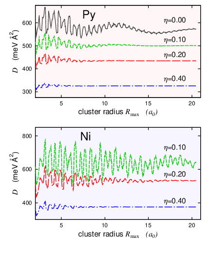
In this section we inspect problems that may be encountered when evaluating the stiffness constant via a weighted sum of the coupling constants , as in Eqs. (8)–(10). Basic understanding can be gained by looking on the dependence of on the maximum distance up to which the individual terms in Eq. (10) are evaluated. This is presented in Fig. 4 for Ni and Py, for several values of the damping parameter . One can see that the quasi-oscillations of extend to quite large distances and that the limiting value depends on the damping parameter .

The stiffness constant is finally determined via . The limit has to be found by extrapolating down to =0. Therefore, one should evaluate for as small as possible. Fig. 4 demonstrates that to evaluate for small , one has to extend the sum in Eq. (10) up to large . Evaluating the exchange coupling constants for large interatomic distances requires a high density of the mesh used for integration in -space [5]. To illustrate this, we present in Fig. 5 the dependence of the constant of Ni on the cut-off distance , for several -space grids. It can be seen immediately that going to larger requires a denser -mesh, increasing dramatically the demand on conputational resources.

The conclusion is thus the following: if we want to evaluate the stiffness constant via Eq. (5), we have to extrapolate to =0, which requires obtaining for small ’s, which requires extending the sum in Eq. (10) to large and that requires a high density for the -mesh. Graphically this is depicted in Fig. 6, where we show how the stiffness constant of Ni and Py depends on the damping parameter , for several choices of the -mesh. The summation in Eq. (10) covers interatomic distances up to . It can be clearly seen that if the parameter is relatively large, the values of do not depend on the -mesh; the situation is numerically stable. However, for small , the values of depend strongly on the -mesh density. Data for cannot be regarded as numerically stable.
| 2nd degree | 3rd degree | 5th degree | |
|---|---|---|---|
| interval | (meV Å2) | (meV Å2) | (meV Å2) |
| 0.2–1.0 | 269.7 | 278.1 | 281.6 |
| 0.4–1.0 | 261.7 | 275.7 | 276.8 |
| 0.6–1.0 | 252.9 | 273.0 | 296.7 |
The fact that the values of obtained for low are not reliable questions the accuracy with which the stiffness constant can be determined. The extrapolation of to =0 is, obviously, a delicate procedure depending on several technical parameters. This is illustrated in Tabs. 8–10 where we show the stiffness constant for Fe, Ni, and Py obtained by extrapolating to using different methods. In particular, the extrapolation was done using a polynomial of the second, third, or fifth degree in , determined by least-squares fitting of when lies in the interval [0.2,1], [0.4,1], or [0.6,1]. The summation Eq. (10) includes all sites up to the distance , which means about 70000 atoms (563 coordination shells) for bcc Fe and about 136000 atoms (773 coordination shells) for fcc Ni and Py. The -space integrals needed to evaluate the constants were carried out on a mesh of points in the full BZ for Fe, points for Ni, and points for Py.
| 2nd degree | 3rd degree | 5th degree | |
|---|---|---|---|
| interval | (meV Å2) | (meV Å2) | (meV Å2) |
| 0.2–1.0 | 708.3 | 754.6 | 768.1 |
| 0.4–1.0 | 663.2 | 736.7 | 769.1 |
| 0.6–1.0 | 618.2 | 712.9 | 785.5 |
One can see from Tabs. 8–10 that the extrapolated values significantly depend on the choice of the fitting interval. The most conclusive estimates of are those obtained using a polynomial fitted to within an interval which includes the smallest usable values for , i.e., [0.2–1.0]. Decreasing the lower boundary of the fitting interval even further is not desirable because the values of may be numerically unstable for (see Fig. 4). As concerns the degree of the polynomial used for the extrapolation: if the extrapolation is done via the second degree polynomial in , the outcome significantly depends on the choice of the interpolating interval. This can hardly be considered as robust or stable. On the other hand, for the fifth degree polynomial, this dependence is only mild. For the third degree polynomial, the situation is somewhere in between. We can thus conclude that estimating the stiffness constant by fitting the dependence by a fifth degree polynomial in leads to trustworthy results.
| 2nd degree | 3rd degree | 5th degree | |
|---|---|---|---|
| interval | (meV Å2) | (meV Å2) | (meV Å2) |
| 0.2–1.0 | 539.4 | 560.6 | 563.1 |
| 0.4–1.0 | 518.5 | 555.1 | 565.4 |
| 0.6–1.0 | 495.9 | 546.1 | 567.6 |

A complementary picture can be obtained by inspecting Fig. 7, where we show the calculated values of for Ni, together with three different polynomial fits of the dependence. Note that if , the values of contain significant numerical errors (see the bottom panel of Fig. 4) — we indicate this by errorbars. The polynomials of the second, third, and fifth degree in were obtained by a least-squares fit for [0.4,1.0]. One can see that the quadratic fit (green dash-dotted line) fails to reproduce outside the fitting range — it significantly deviates from the values marked by open circles in Fig. 7. The situation is better for the cubic fit. The best outcome is apparently achieved if the fit is done by a fifth-degree polynomial.
III.3 Direct evaluation of in reciprocal space
The third way to calculate the spin wave stiffness constant is via integrating the relevant expression in reciprocal space, according to Eq. (11). As this is a direct evaluation, no analysis of the fitting or extrapolation procedure is needed. The values we obtained from Eq. (11) are given in the fourth column of Tab. 11.
IV Discussion
Our goal was to critically review different approaches to calculate the spin wave stiffness constant and to compare the results calculated for selected systems on the same footing. The approaches we investigated include (i) examining the long-wave-length behavior of the spin wave energy dispersion [see Eqs. (3) and (7) and Sec. III.1], (ii) evaluating a weighted sum of exchange coupling constants [Eqs. (8)–(10) and Sec. III.2], and (iii) direct evaluation of Eq. (11) in reciprocal space. The results for Fe, Ni, and Py obtained by these methods are summarized in Tab. 11. The errors were estimated by considering the -mesh convergence (for all three cases) and, additionally, considering the ambiguity of finding the right fits for in case of analysis of the spin wave energy dispersion (see Tabs. 5–7) and of extrapolating to in case of the summation in real space (see Tabs. 8–10). A minor contribution to the errors comes also from the limit when determining and from having a finite when determining . These last two contributions are quite small in comparison with the errors due to the ambiguity of the fitting and/or extrapolating procedure.
| from | from | from | |
|---|---|---|---|
| Fe | 3022 | 2792 | 2623 |
| Ni | 7474 | 7686 | 7817 |
| Py | 5211 | 5632 | 5125 |
Small but distinct differences are evident in Tab. 11, even though all the approaches use very similar physical assumptions. In particular, in all cases it is assumed that the magnetization direction can be described by vectors pinned to atomic sites [3; 4]. All calculations have been performed within the same KKR Green function formalism, using the sprkkr code, ensuring that the quantities used in different approaches (coupling constants, spin wave energies) are consistent.
To point out the differences in the approaches used here, we start by noting that the scalar relativistic spin spiral calculations are performed selfconsistently for each wave vector . As a consequence, the exchange splitting of the energy bands as well as the local magnetic moments are -dependent. Moreover, the spin-spiral energy has been evaluated based on the total energy of the system. The other two approaches, i.e., the methods based on the real-space summation according to Eqs. (8)–(10) and on the reciprocal space integral according to Eq. (11), rely on the magnetic force theorem and assume that the magnitude of the magnetic moments does not change if they are tilted (rigid spin approximation). These two approaches are formally equivalent, as it was shown, e.g., by Liechtenstein et al. [3]. However, small differences in the results occur because the approaches lay different requirements concerning the accuracy of numerical calculations. The requirements laid by the real-space approach are discussed above in details. The approach based on the Brillouin-zone integration is very sensitive to the features of the electronic structure because of the -derivatives of the -matrix in Eq. (11), in contrast to the real-space approach. As a result, a very dense -mesh is needed for the BZ-integration to achieve convergence with respect to the number of -points.
The effect of using the magnetic force theorem can be seen from the data in Tabs. 2–4: it may result in errors of few percents. The assumption that the magnetic moments do not change their magnitude if there are tilted is plausible for the systems we are dealing with (see, e.g., Ref. [9] or lower panels of Figs. 1–2), nevertheless, small differences still may occur because of this.
| work | Fe | Ni | Fe1-xNix | |
|---|---|---|---|---|
| [25] (1964) | 325 | 400 | 400 | 80 |
| [26] (1966) | 350 | |||
| [27] (1968) | 314 | 470 | ||
| [28] (1973) | 555 | |||
| [29] (1973) | 311 | |||
| [30] (1975) | 525 | 335 | 68 | |
| [31] (1975) | 555 | |||
| [32] (1976) | 390 | |||
| [33] (1977) | 398 | |||
| [34] (1981) | 593 | |||
| [35] (1982) | 270 | 413 | ||
| [36] (1983) | 530 | 390 | 80 | |
| [37] (1984) | 307 | |||
| [38] (1985) | 398 | |||
| [39] (2017) | 440 | 80 |
As a whole, the differences between the values of obtained for identical systems by different methods seem to be larger than what could be ascribed to “numerical noise”. A closer look at Tabs. 5–7 in Sec. III.1 and Tabs. 8–10 in Sec. III.2 reveals that use of just a bit different fitting and extrapolation method can give rise to differences of 5–10 %. Even though we put a lot of effort to compensate for ambiguities, some issues probably remained. The third approach does not require any fitting or extrapolation but it requires a very dense -mesh to get truly converged results for the spin-wave stiffness, making the calculations very demanding. We assume that the results obtained by means of Eq. (11) could still be improved upon by increasing the -mesh density but only at very high (impractical) computational costs.
On the other hand, possible errors of the procedures to calculate concern mostly the absolute values, not the trends. For example, application of the real-space summation Eqs. (8)–(10) to Py doped with V, Gd, and Pt led to a good theoretical description of the way the dopants influence the spin wave stiffness, in agreement with experiment [20]. Likewise, the dependence of the spin wave stiffness of the Fe1-xNix alloy on its composition can be properly described both by fitting the spin wave energy dispersion according to Eqs. (3) and (7) and by direct evaluation of via a reciprocal-space integral according to Eq. (11) [14].
Uncertainty in determining the theoretical values of the stiffness constants for Fe, Ni, and Py is accompanied by uncertainty in experiment. We summarize in Tab. 12 a selection of available experimental data; a more complete list can be found, e.g., in Tables 7 and 8 of Vaz et al. [1]. One can see that the spread of results of different studies is quite large — about 15 % for Fe and Py and about 20 % for Ni. A critical assessment of experimental studies is beyond our scope. Despite the relatively large spread of the data, Tabs. 11–12 indicate that our theory agrees well with experiment for Fe, whereas for Ni and Py the agreement is less good. Tentatively this is linked to problems with describing the exchange coupling of Ni in terms of the coupling constants [40; 41]. Some errors could be also introduced because of the restrictions of our computational scheme, notably the ASA; nevertheless, full-potential effects are usually small in close-packed metals such as those we are dealing with. It is more likely that the assumption of rigid moments is not fully justified for Ni and its alloys.
Even though our study has been performed for Fe, Ni, and Py, it is focused on analyzing and discussing concepts that have to be dealt with when studying the spin wave stiffness for any material. Metallic systems such as those we investigate here represent the most difficult case as concerns evaluating the stiffness by means of a weighted sum of the coupling constants (Sec. III.2). This is because for metals the coupling constants decay with distance as [5], i.e., relatively slowly. For semiconductors and insulators, the opening of a gap leads to an exponential decay of the exchange coupling, as [5; 42], improving the convergence of the expression Eq. (5) considerably. This will enable to employ larger and lower , possibly disposing of the damping term altogether. Increasing the disorder (as, for example, in the case of high-entropy alloys) will introduce an exponential spatial damping of the exchange coupling as well [42].
The analyses performed in Sec. III enable us to draw some recommendations how to evaluate the stiffness constant . In general, evaluating by means of fitting by a polynomial is less demanding and more reliable than evaluating by means of extrapolating obtained by means of summation. The convergence with the -mesh density is better in the former case and, moreover, extrapolation required in the latter case is always an ambiguous procedure. However, fitting by a polynomial to determine the coefficient at the quadratic term is not without risks either. Higher powers should be included in the fitting polynomial Eq. (17); employing just a simple quadratic fit as done, e.g., in [43] may not always be sufficient.
In many cases, calculating the energy dispersion is difficult or impractical (e.g., for multicomponent systems with substitutional disorder). Extrapolating down to then remains the only viable option. In such cases, extra care has to be taken and the robustness of the selected extrapolation procedure should be checked. For example, application of a quadratic extrapolation within the [0.6,1.0] interval (employed, e.g., for transition metals [5] or for Heusler alloys [18]) to the systems investigated here would lead to a systematic undershooting of by about 10 %. Of course, these conditions have to be explored specifically for each system considered. Evaluating directly in reciprocal space Eq. (11) does not suffer from the pitfalls of fitting or extrapolating but it is numerically demanding and sensitive to the details of the electronic structure.
V Conclusions
Evaluating the spin wave stiffness constant by current schemes is technically difficult and potentially numerically unstable. Differences between values obtained by different methods of 5–10 % remain even if care is taken to make all the calculations consistent with each other and well converged. The agreement between theoretical values and experimental data is good in case of Fe but significant differences occur for Ni and permalloy Fe0.19Ni0.81.
Calculating the stiffness constant usually involves either fitting the long-wave-length part of the spin wave energy dispersion by a polynomial, or extrapolating the values obtained via a real-space summation of weighted exchange coupling constants to zero damping, . Both procedures are tricky and quite sensitive to technical details how the fitting or extrapolation is done.
Acknowledgements.
This work was supported by the GA ČR via the project 17-12925S and by the Ministry of Education, Youth and Sport (Czech Republic) via the project CEDAMNF CZ.02.1.01/0.0/0.0/15_003/0000358. Additionally, financial support by the DFG via Grant No. EB154/36-1 is gratefully acknowledged.References
- Vaz et al. [2008] C. A. F. Vaz, J. A. C. Bland, and G. Lauhoff, Rep. Prog. Phys. 71, 056501 (2008).
- Kübler [2000] J. Kübler, Theory of Itinerant Electron Magnetism, International Series of Monographs on Physics (Oxford University Press, Oxford, 2000).
- Liechtenstein et al. [1984] A. I. Liechtenstein, M. I. Katsnelson, and V. A. Gubanov, J. Phys. F: Met. Phys. 14, L125 (1984).
- Liechtenstein et al. [1987] A. I. Liechtenstein, M. I. Katsnelson, V. P. Antropov, and V. A. Gubanov, J. Magn. Magn. Materials 67, 65 (1987).
- Pajda et al. [2001] M. Pajda, J. Kudrnovský, I. Turek, V. Drchal, and P. Bruno, Phys. Rev. B 64, 174402 (2001).
- Yu et al. [2008] P. Yu, X. F. Jin, J. Kudrnovský, D. S. Wang, and P. Bruno, Phys. Rev. B 77, 054431 (2008).
- Pan et al. [2017] F. Pan, J. Chico, A. Delin, A. Bergman, and L. Bergqvist, Phys. Rev. B 95, 184432 (2017).
- Mryasov et al. [1996] O. N. Mryasov, A. J. Freeman, and A. I. Liechtenstein, J. Appl. Phys. 79, 4805 (1996).
- Rosengaard and Johansson [1997] N. M. Rosengaard and B. Johansson, Phys. Rev. B 55, 14975 (1997).
- Brown et al. [1999] R. H. Brown, D. M. C. Nicholson, X. Wang, and T. C. Schulthess, J. Appl. Phys. 85, 4830 (1999).
- van Schilfgaarde and Antropov [1999] M. van Schilfgaarde and V. P. Antropov, J. Appl. Phys. 85, 4827 (1999).
- Morán et al. [2003] S. Morán, C. Ederer, and M. Fähnle, Phys. Rev. B 67, 012407 (2003).
- Shallcross et al. [2005] S. Shallcross, A. E. Kissavos, V. Meded, and A. V. Ruban, Phys. Rev. B 72, 104437 (2005).
- Mankovsky et al. [2019] S. Mankovsky, S. Polesya, and H. Ebert, Phys. Rev. B 99, 104427 (2019).
- Ebert et al. [2011] H. Ebert, D. Ködderitzsch, and J. Minár, Rep. Prog. Phys. 74, 096501 (2011).
- Ebert [2014] H. Ebert, The sprkkr package version 7, http://olymp.cup.uni-muenchen.de/ak/ebert/SPRKKR (2014).
- Mankovsky et al. [2011] S. Mankovsky, G. H. Fecher, and H. Ebert, Phys. Rev. B 83, 144401 (2011).
- Thoene et al. [2009] J. Thoene, S. Chadov, G. Fecher, C. Felser, and J. Kübler, J. Phys. D: Appl. Phys. 42, 084013 (2009).
- Dürrenfeld et al. [2015] P. Dürrenfeld, F. Gerhard, J. Chico, R. K. Dumas, M. Ranjbar, A. Bergman, L. Bergqvist, A. Delin, C. Gould, L. W. Molenkamp, and J. Åkerman, Phys. Rev. B 92, 214424 (2015).
- Šipr et al. [2019] O. Šipr, S. Mankovsky, and H. Ebert, Phys. Rev. B 100, 024435 (2019).
- Ebert et al. [1996] H. Ebert, H. Freyer, A. Vernes, and G.-Y. Guo, Phys. Rev. B 53, 7721 (1996).
- Šipr et al. [2014] O. Šipr, S. Bornemann, H. Ebert, and J. Minár, J. Phys.: Condens. Matter 26, 196002 (2014).
- Šipr et al. [2016] O. Šipr, S. Mankovsky, S. Polesya, S. Bornemann, J. Minár, and H. Ebert, Phys. Rev. B 93, 174409 (2016).
- Terakura et al. [1982] K. Terakura, N. Hamada, T. Oguchi, and T. Asada, J. Phys. F: Met. Phys. 12, 1661 (1982).
- Hatherly et al. [1964] M. Hatherly, K. Hirakawa, R. D. Lowde, J. F. Mallett, M. W. Stringfellow, and B. H. Torrie, Proceedings of the Physical Society 84, 55 (1964).
- Phillips [1966] T. G. Phillips, Proc. Roy. Soc. (London) A 292, 224 (1966).
- Stringfellow [1968] M. W. Stringfellow, J. Phys. C: Solid State Phys. 1, 950 (1968).
- Mook et al. [1973] H. A. Mook, J. W. Lynn, and R. M. Nicklow, Phys. Rev. Lett. 30, 556 (1973).
- Riedi [1973] P. C. Riedi, Phys. Rev. B 8, 5243 (1973).
- Hennion et al. [1975] M. Hennion, B. Hennion, A. Castets, and D. Tocchetti, Solid State Commun. 17, 899 (1975).
- Aldred [1975] A. T. Aldred, Phys. Rev. B 11, 2597 (1975).
- Maeda et al. [1976] T. Maeda, H. Yamauchi, and H. Watanabe, J. Phys. Soc. Jpn. 40, 1559 (1976).
- Riedi [1977] P. Riedi, Physica B+C 91, 43 (1977).
- Lynn and Mook [1981] J. W. Lynn and H. A. Mook, Phys. Rev. B 23, 198 (1981).
- Pauthenet [1982] R. Pauthenet, J. Appl. Phys. 53, 2029 (1982).
- Nakai [1983] I. Nakai, J. Phys. Soc. Jpn. 52, 1781 (1983).
- Loong et al. [1984] C. Loong, J. M. Carpenter, J. W. Lynn, R. A. Robinson, and H. A. Mook, J. Appl. Phys. 55, 1895 (1984).
- Mitchell and Paul [1985] P. W. Mitchell and D. M. Paul, Phys. Rev. B 32, 3272 (1985).
- Yin et al. [2017] Y. Yin, M. Ahlberg, P. Dürrenfeld, Y. Zhai, R. K. Dumas, and J. Åkerman, IEEE Magnetics Letters 8, 1 (2017).
- Bruno [2003] P. Bruno, Phys. Rev. Lett. 90, 087205 (2003).
- Kudrnovský et al. [2008] J. Kudrnovský, V. Drchal, and P. Bruno, Phys. Rev. B 77, 224422 (2008).
- Kudrnovský et al. [2004] J. Kudrnovský, I. Turek, V. Drchal, F. Máca, P. Weinberger, and P. Bruno, Phys. Rev. B 69, 115208 (2004).
- dos Santos et al. [2017] F. J. dos Santos, M. dos Santos Dias, and S. Lounis, Phys. Rev. B 95, 134408 (2017).