Driving Quantum Correlated Atom-Pairs from a Bose-Einstein Condensate
Abstract
The ability to cool quantum gases into the quantum degenerate realm has opened up possibilities for an extreme level of quantum-state control. In this paper, we investigate one such control protocol that demonstrates the resonant amplification of quasimomentum pairs from a Bose-Einstein condensate by the periodic modulation of the two-body -wave scattering length. This shows a capability to selectively amplify quantum fluctuations with a predetermined momentum, where the momentum value can be spectroscopically tuned. A classical external field that excites pairs of particles with the same energy but opposite momenta is reminiscent of the coherently-driven nonlinearity in a parametric amplifier crystal in nonlinear optics. For this reason, it may be anticipated that the evolution will generate a ‘squeezed’ matter-wave state in the quasiparticle mode on resonance with the modulation frequency. Our model and analysis is motivated by a recent experiment by Clark et al. that observed a time-of-flight pattern similar to an exploding firework [1]. Since the drive is a highly coherent process, we interpret the observed firework patterns as arising from a monotonic growth in the two-body correlation amplitude, so that the jets should contain correlated atom pairs with nearly equal and opposite momenta. We propose a potential future experiment based on applying Ramsey interferometry to experimentally probe these pair correlations.
1 Introduction
The ability to tune the two-body scattering length in a Bose-Einstein Condensate (BEC) by varying the magnitude of a magnetic field in the vicinity of a Feshbach resonance has been employed in a number of seminal experiments that aim to investigate controlled non-equilibrium quantum dynamics. One such example is the so-called ‘Bosenova’ experiment by Donley et al. [2], in which a BEC was subject to a sudden change of the scattering length from a small positive value to a large negative value. This resulted in a change of the sign of the mean-field interactions from repulsive, where the gas is mechanically stable, to attractive, where the compressibility may be negative and the gas is then unstable [3]. What was observed experimentally after this abrupt change in the scattering length was a collapse and subsequent explosion of the quantum gas in a manner that resembled an astrophysical supernova. Theoretical models were subsequently developed and illustrated that the emergence of a pairing field in the underlying quantum many-body system can explain the observed burst of non-condensate atoms [4].
More recently, Bose ‘firework’ experiments [1] have observed pairs of high momentum atoms emitted as jets from a condensate driven by a periodic modulation of the two-body -wave scattering length. These experiments demonstrated a protocol for resonantly amplifying quantum fluctuations with well-controlled momenta when starting from a stationary BEC. The fact that the jets were observed to be correlated in emission direction motivates us to consider whether the many-body pairing field played an important role in the dynamics, in a similar manner to the Bosenova system previously studied. This aspect is related to other calculations that explore the second order coherence of the gas [5].
In the case of a dilute quantum gas, the Gross-Pitaevskii equation (GPE) provides an accurate description of the equilibrium and time-dependent behavior of the BEC. In this framework, the interacting condensate is completely described by a mean-field superfluid order parameter. The GPE framework has been extensively applied to model the behavior of BECs at zero temperature, and also to their coherent manipulation through externally applied potentials. However, when there is a significant portion of non-condensate atoms, the GPE will fail to provide an accurate description of the system. A small amount of non-condensate atoms is always present even at zero temperature in a dilute quantum gas arising from the beyond mean-field fluctuations that are due to the finite interaction strength. It is of course possible to generate substantial fractions of non-condensate atoms by driving a pure condensate in a variety of ways, and this is typically unavoidable when the currents that generate the magnetic confinement fields contain stochastic noise. Furthermore, non-condensate atoms are always present in systems with finite temperature since they embody the thermal excitations. In order to capture the essential dynamics associated with the non-condensed component, a theory that goes beyond the mean-field approximation is necessary.
A systematic extension to the simplest mean-field approach given by the GPE is the Hartree-Fock Bogoliubov (HFB) formalism that takes into account the interactions between three components. We will refer to these as the condensate, the non-condensate, and the pairing field of the fluctuations. In this formalism, the elementary excitations are described as Bogoliubov quasiparticles [6], and the ground state condensate is a vacuum of such quasiparticles. The quasiparticle creation operator is a linear combination of the atom creation operator (particles) and the atom annihilation operator (holes). The vacuum state due to interactions possesses a portion of non-condensate atoms referred to as quantum depletion. The recent ‘firework’ experiments that tune the scattering length by applying an appropriate external magnetic field potentially allow all of these components—the mean-field, non-condensate, and pairing field—to be controlled, manipulated, and engineered. In this paper we derive the solutions of the HFB theory as applied to well-controlled experimental geometries in order to determine the efficacy of this framework for providing a theoretical basis for the recent observations.
One approach for describing collective excitations of a condensate involves solving the Bogoliubov de Gennes equations [7], which is most accurate when the excitations are weak. When the excitations are not weak, and the non-condensate fraction can be significant, a more complete approach must be used such as the time-dependent self-consistent HFB equations [8], and that is the method we will focus on in this paper. Note that one alternative approach that can incorporate the excitations is through the addition of a noise source to introduce fluctuations directly into the Gross-Pitaevskii equation [9]. However, this assumes by construction that the many-body state can be accurately described by a unique macroscopic wavefunction, and therefore a more complete theory is needed to describe two-body correlations.
We emphasize the importance of the pairing field in our analysis. Pairing gives rise to an anomalous density that allows us to investigate the coherence of the system and explore methods to probe phase-sensitive quantities. However, to incorporate the pairing field in our simulations requires a number of important considerations. Since our modeling assumes contact interactions, numerical studies have to account for the potentially divergent nature of the pairing field at both short and long length scales by appropriate renormalization of the scattering potential. We demonstrate how to renormalize the scattering potential when momentum is represented on a discrete grid. Furthermore, when solving for the initial condition of the system, instead of using an approximation that ignores the pairing field [10] in order to remedy issues associated with the gapless energy spectrum, we take an alternative approach in which the condensate, depletion and pairing field are accounted for and we solve for the HFB theory self-consistently.
Note that there is one other important consideration; our model does not include the collisions terms in the kinetic theory that result in equilibration of the gas to its thermal state [11]. Neglecting collisions is a good approximation for a dilute gas at low temperature, but implicitly requires us to limit our discussion to the regime in which the time-scale between consecutive two-body collision events greatly exceeds the time-scale of the quantum dynamics that we investigate. Finally, all this has to be implemented in multiple dimensions in order to provide a useful comparison with experimental observations.
The paper is outlined as follows. We present the model in Section 2 and provide details of the renormalization process in Section 3. At first we limit our discussion to the most straightforward case of quasi-1D systems. In Section 4, we outline the numerical procedures necessary to obtain a self-consistent ground state solution to the HFB theory for a weakly-interacting trapped quantum gas, and quantify the quantum depletion as well as the pairing field amplitude. In Sections 5 and 6, we use the time-dependent HFB theory to show that the modification of the interaction strength through modulation of the scattering length parametrically amplifies a certain quasiparticle mode and generates a matter-wave solution that is analogous to a squeezed state of light. In Section 7, we use these results to explore the possibility of future experiments that utilize interferometry to probe the pair correlation amplitude. We consider two methods that create a phase difference between the driving field and the pairing field, and consequently lead to the possibility for constructive and destructive interference in the matter-wave density. Finally, in Section 8, we extend the results to quasi-2D so that they can be compared with the experimental observations of angular correlations in the firework pattern, where the atoms were confined in a pancake-shaped confining potential well and were ballistically expanded.
2 General many-body field theory
We begin from the many-body Hamiltonian that describes a weakly interacting Bose gas with pairwise contact interactions:
| (1) | |||||
where is the mass of the atom and is the external trapping potential. The field operators, and , are bosonic operators that annihilate and create particles and obey commutation relations . The strength of the interaction potential, , is related to the -wave scattering length, , by , where is the three-dimensional -matrix (here it is actually a simple scalar and not a matrix since we consider the regime in which there is no dependence of the scattering phase shift on energy) and is the dimensionless renormalization factor that will be fully discussed in Section 3.
Since we intend to explore excitations from a BEC, we assume that the field operator is well described by a mean field amplitude describing the atom condensate, , and a fluctuating component, i.e.,
| (2) |
where . The second-order terms—normal and anomalous densities—are defined respectively as,
| (3) |
Both of these play an important role in the dynamics of the non-condensate component of the system we are interested in. In particular, the diagonal elements of the normal density, , represent the physical non-condensate atom densities at position and are therefore positive semi-definite. The off-diagonal elements represent the matter-wave correlations of the non-condensate atoms that are characterized by quantities such as the de Broglie wavelength and effective temperature. The anomalous density, , is the pairing field that characterizes the two-particle correlations in the system.
If we assume that the the field fluctuations are Gaussian, one can drop the third-order cumulants, and expand the fourth-order quantities in terms of the second-order cumulants when deriving the evolution equations. In practice, this involves repeated application of Wick’s theorem [12]. The resulting equations of motion are closed and can be written in detail for the condensate as;
| (4) | |||||
for the normal density as;
| (5) | |||||
and for the anomalous density as;
| (6) | |||||
Here we have simplified the notation by introducing two energy functionals,
| (7) |
for the single-particle self-energy and the gap, respectively. Due to the fact that we neglect explicit three-particle and higher correlations, the validity of this approach is restricted to the dilute gas regime. Note that equation (4) can simplified to the Gross-Pitaevskii equation if terms involving and are dropped. In this case, the time-independent energy eigenvalue represents the chemical potential, , so that . The delta function in equation (6) arises from the bosonic commutation relation of the field operators and can therefore be interpreted as a quantum effect. A number of quantities are conserved in this evolution; in particular, the total atom number
| (8) |
is invariant under time evolution governed by equations (4)–(7).
In order to see how the anomalous density is related to the vacuum pair wavefunction for the interatomic separation of two atoms, we may neglect the mean-field density and the normal density in equation (6), and then the eigenvalue equation is simplified to
| (9) |
where . equation (9) can be identified as a one-dimensional Schrödinger equation of a fictitious particle of reduced mass scattering off a potential . Then is interpreted as the resulting eigenstate wavefunction corresponding to the familiar two-particle scattering solution of the equation written in terms of the relative coordinate.
3 Renormalization of the Scattering Potential
The Dirac delta function in equation (9) implies that we are implicitly building a scattering model from a contact interaction. This is convenient as it simplifies the resulting field theory, but care must be taken to account for divergences that can arise at small and large scales. In general, this is remedied by renormalization of the potential strength. In order to carry out this renormalization procedure, we begin from the formal scattering theory [13], where we define the bare scattering potential operator, , which has units of energy, and thereby expand the -matrix in an order-by-order series;
| (10) | |||||
Here is the bare single particle propagator,
| (11) |
the scattering energy is , the dispersion relation is with the momentum, and we need to implicitly consider the limit . The -matrix elements are , where is the wavenumber basis state. For the low energy scattering limit, the -matrix becomes independent of , and does not depend on or . In this case the -matrix is well characterized by a constant scalar associated with the -wave scattering length, as mentioned earlier, i.e., .
Further considerations have to be made when one or more dimensions are effectively frozen out due to imposing a strong confining potential in these dimensions. Without loss of generality, let us consider the strong confining potential to be a harmonic potential with oscillator length given by . If one dimension is frozen out, an effective quasi-2D geometry is realized, and if two dimensions are frozen out, an effective quasi-1D system is generated. If we denote the number of free dimensions by , the appropriate -matrix expression, , for the reduced dimensional case can be related recursively by and [14][15].
The process of renormalization connects the -matrix, , to the strength of the potential, , by expanding equation (10) in the momentum basis, and this connection depends on the dimensionality of the system,
| (12) |
where the critical element here is the introduction of and as infrared and ultraviolet momentum cutoffs, respectively. The cutoffs have to be chosen from an appropriate asymptotic limit in order to accurately capture the dynamics of interest. The renormalization procedure can be represented by the introduction of a parameter, , defined by solving equation (12) for . This gives the solution,
| (13) |
where
| (14) |
In order to illustrate the behavior of , we consider the solution to scattering equation, equation (9), where the stationary energy eigenvalue is and the mass is replaced by the reduced mass of two particles, . Solving this system of equations has a character that depends on the dimensionality. In three dimensions, we may set , and perform the integral to give for a particle scattering at low energy, [16]. In 2D, the integral scales logarithmically and has both ultraviolet and infrared divergences. In 1D, there is an infrared divergence so must be non-zero but we may set to infinity.
We do not provide all the details here, since, in practice, these are formal considerations that do not actually affect our numerical simulations. Indeed there are actually no divergences introduced that require the introduction of momentum cutoffs to rectify when the momenta are restricted to values on discrete and finite grids. This is always the case in a numerical computer model that aims to describe a realistic experiment. In such a discrete representation of possible momenta, it is preferable to simply calculate a finite sum over a specific partition instead of evaluating the continuous integral analytically. This implies a numerical evaluation of , giving , and therefore determining for a given -matrix, which replaces in the HFB equations, i.e., equations (4)–(6). Here the subscripts label individual discrete momenta, and thus represents the momentum grid, with is the total number of grid points.
We carry out this renormalization procedure for all the results that we present in this paper. For each calculation, we verify that the numerical results are independent of the details of the momentum grid on which the field theory is represented.
4 Self-consistent ground state solution
In order to find a self-consistent solution to prepare an initial condition for the subsequent time evolution, the first step will be to consider the non-condensate component to be absent, and to find a ground state representation of the condensate by solving the GPE. We then use this condensate field as input into the time-independent equations for the normal and anomalous densities, and diagonalize the resulting HFB self-energy matrix to find the quasiparticle basis. As we will see, this process exhibits a defect in the zero-energy subspace (i.e., the eigenvectors do not span the space). The intepretation is that the eigensolution is not stationary and cannot be used as an accurate description of the initial condition for subsequent time evolution. We therefore reintroduce the non-condensate terms that we have just found into the equations for the condensate, normal density, and anomalous density and solve again the system of equations, giving rise to an iterative method that generates an accurate self-consistent initial condition.
Our approach will be to begin by first fully describing the necessary procedure using the simple case of quasi-1D where the problem is most easily tractable. However, higher dimensions can be treated in a similar method to the manner we present (we will consider quasi-2D later in Section 8). The reduction to one-dimensional behavior requires the transverse confinement condition
| (15) |
to be satisfied, where is the one-dimensional density [17][18], and as defined previously, is the harmonic oscillator length in the two strongly confining directions, here assumed to be equal.
The first part of our numerical algorithm is to solve for the ground state of the GPE,
| (16) |
We use imaginary-time propagation to derive the lowest energy solution and its energy eigenvalue representing the associated chemical potential. Then, the mean field solution, , can be used as a parameter to construct the self-energy matrix;
| (17) |
where
| (18) |
The self-energy matrix has dimensionality where is the size of the single particle basis, as defined previously. This energy operator is most simply expressed in the position basis, where , since in that representation the potential terms including the mean-field appear as diagonal blocks. The eigenstates of are the Bogoliubov quasiparticles. Since the matrix satisfies , where , the eigenenergies come in pairs of positive and negative values, , and the corresponding eigenstates are and . The eigenstates are normalized by satisfying the constraint
| (19) |
Although this construction may appear standard and straightforward, there is a well-known and implicit subtlety when examining the solutions to this eigensystem. When investigating the zero-energy eigensolutions, one finds a pair of eigenstates that are colinear (equal up to a multiplicative scalar) that have the form . This solution creates two significant issues. First, the colinear eigenstates cannot be normalized by equation (19). Second, they do not span the two-dimensional subspace of the Hilbert space corresponding to zero-energy.
The origin of this mathematical fact has an intuitive explanation. It arises from the approximations that lead to this self-energy matrix, that is, by fixing the condensate solution as an unchanging parameter, one builds an unphysical model that implicitly allows the unconstrained growth of a zero energy mode as a function of increasing time. Consequently there is no stationary solution. This has to be remedied, for example, through a self-consistent approach in which the condensate is treated as a variational parameter, in order to allow us to extend the formalism so that it may be applied to our system of interest.
We begin by determining the remaining eigenvector to fully span the zero-energy subspace by employing the Gram-Schmidt orthogonalization method to numerically calculate the remaining basis vector. In this way we determine an eigenvector solution such that for all , and normalize it to [19]. The addition of this vector to the eigenvectors of the self-energy completes the basis of the vector space. The reason that this is important is that it allows the field operator to be expanded as
| (20) |
where and are bosonic annihilation and creation operators for the quasiparticles. We have introduced and as a pair of canonically conjugate operators that fully describe the zero-energy mode and obey the cannonical commutation relation , .
It is convenient to identify two special combinations of and in order to give a concise expression for the completeness relation. We define , along with the matrix
| (21) |
so that the following completeness relation is satisfied;
| (22) |
This allows the particle annihilation operator to be written as
| (23) |
where the sum is over the elements of the index set , and is the annihilation operator for the zero-energy mode given by .
At this point, we have determined the quasiparticle basis, and can populate that basis with a given set of probabilities in order to generate particle distributions. In particular, we would like to derive the normal and anomalous densities that are essential elements of the HFB theory. To begin with we construct the Hermitian density matrix:
| (24) | |||||
where the population matrix has the form
| (25) |
The diagonal elements of are the populations of each quasiparticle , and the off-diagonal elements represent the correlations between different quasiparticles. In the ground state, and . The identity, , on the lower-right block is interpreted as a bosonic analog to the Dirac sea [20], in which the negative energy states are occupied by boson holes. When there is an excitation, a pair of one particle and one hole is created, and therefore appears in both the upper-left and the lower-right block, as shown in equation (25).
This formalism now allows an extremely concise representation of the full dynamical evolution encapsulated in equations (5) and (6);
| (26) |
where is defined according to equation (24). The consequence of completing the basis by establishing the missing eigenvector through Gram-Schmidt orthogonalization is now evident. If we begin with the bare , as defined in equation (17) and initialize to the ground state (meaning and ) of the corresponding eigenbasis, then when equation (26) is propagated from this initial condition, it is evident that the solution is not stationary. The number of non-condensate atoms is seen to grow as , as shown in Fig. 1. This implies that we have not in fact determined the correct ground state.

This problem arises because, using the language of quantum optics, we are effectively assuming that the condensate is a coherent field that may act as an infinite classical pump and can provide a reservoir source for introducing an infinite number of atom-pairs. Furthermore, it does not cost any energy to introduce a zero-energy quasiparticle within this framework. This is clearly unphysical for a number of reasons including the fact that, as can be seen in equation (4), the factor of two in front of the interaction between the condensate and the non-condensate atoms means that it actually costs energy to take away atoms from the condensate and move them into the non-condensate fraction, providing the interactions are repulsive (scattering length positive). There is some literature that suggests simply dropping the zero-modes entirely to remedy this problem, for example, Ref. [21]; however, this generally violates the fundamental commutation relations of the bosonic field operator and therefore the uncertainty principle, so we do not employ that approach here.
We instead employ an alternative solution by including the second-order terms to generalize the self-energy matrix. This means that we modify equation (18) to include the effects of the normal and anomalous densities, and then introduce the renormalization of the -matrix to give
| (27) |
with both equation (17) and equation (26) unmodified. In order to be consistent, however, we must also generalize the GPE, equation (16), to
| (28) | |||||
Note that the ground state solution of the GPE is stationary, and thereby determines the value of the chemical potential that enters the renormalization (see Section 3). Since and are functionally dependent on the eigenstates themselves, the problem is nonlinear, and it is necessary to solve the generalized self-energy, equation (27), and the generalized GPE, equation (28), iteratively until the equations are self-consistent [22]. We point out that this iterative process will typically create a small gap in the energy spectrum of the system around zero energy, and the problem of the unphysical non-stationary eigensolution that is caused by the zero-energy subspace is no longer present. The resulting self-consistent solution is stationary under the evolution given by equation (26) and provides an accurate ground state initial condition for the subsequent time-dependent simulations that we present in the rest of the paper.
5 Dynamics of the time-dependent HFB system
In the experiment by Clark et al. [1], an external sinusoidally oscillating magnetic field is applied, and therefore the scattering length is modulated in the form
| (29) |
where is the initial scattering length, and is the amplitude of the oscillating component of the scattering length at angular frequency . The dynamics of the system under this modulation is interesting to consider because the oscillating external field will inject energy into the system, and this will result in exciting atoms from the ground state into higher quasiparticle levels.
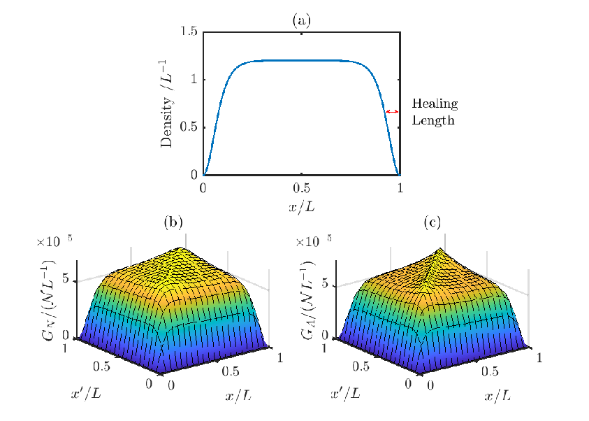
We begin our simulations by preparing the system in the self-consistent ground-state of the HFB theory for a small positive value of the scattering length using the procedure just described. An illustration of the resulting condensate, normal and anomalous densities are shown in figure 2. After preparing the system in the ground state, we solve equation (17) and equation (26) using the generalized equations (27) and (28) with a sinusoidal modulation of the scattering potential, i.e.,
| (30) |
In order to interpret our results, we display the occupation probabilities via the projection of onto the initial quasiparticle basis found from the self-consistent HFB Hamiltonian at time . The procedure is as follows. Since the quasiparticle eigenbasis matrix, , satisfies , we may write
| (31) |
Then, according to equation (24),
| (32) | |||||
where is the original self-consistent quasiparticle basis determined for the initial condition. The resulting population is shown in figure 3. The height of the peak in the off-diagonal block (i.e., ) is notable since the coherence saturates the upper bound of the Cauchy-Schwartz inequality,
| (33) |
which in turn can be interpreted as confirming that the process of exciting quasiparticles from the condensate is maximally coherent. The diagonal elements, , can be measured by time of flight, since the quasiparticles transform into regular particles that can be detected during ballistic expansion. In other words, when the kinetic energy greatly exceedes the interaction energy, the ’s then effectively label the free momentum, i.e., .


As shown in figure 3, when the periodic drive is turned on continuously for many cycles, essentially only one quasiparticle mode is resonantly amplified. That is consistent with the narrow spectrum. This physical process can be interpreted as being due, as a consequence of the oscillating drive, to a photon with energy being absorbed by a pair of atoms, with each of them getting half the energy, . In addition, the phonon-like collective excitations that correspond to the observed wave-like patterns seen in the condensate density can be interpreted as the Faraday patterns that typically manifest in different kinds of parametrically driven fluids [23]. The pattern resembles the wavefunction density for the single quasiparticle mode on resonance. This simulation illustrates that by careful engineering of the drive, one can potentially prepare a variety of quantum states, selectively exciting atoms from the condensate field. We now show a few illustrative examples of interesting cases that employ this technique.
6 Dynamically Generating Squeezed Quasiparticle States
A squeezed state refers to a quantum state that has a reduced uncertainty in one degree of freedom (‘squeezed’) at the expense of increased uncertainty in a canonically conjugate variable [24, 25, 26, 27, 28, 29, 30]. Such states have been extensively studied in quantum optics and atomic physics due to their utility in quantum metrology for producing measurement precision that exceeds the limits derived from classical states. Here we will show how to use the resonant quasiparticle excitation in order to generate a squeezed matter-wave state, anticipating that this could potentially be applied to quantum matter-wave interferometry.
By driving the system resonantly, we are effectively producing resonant pairs with well defined energy, and this is reminiscent of nonlinear optical devices that down-convert pump photons into signal and idler pairs. Here we will demonstrate that this correspondence is robust and quantitative by demonstrating how one may calculate the squeezing parameter associated with the analogous quantity that is regularly computed in the quantum description of light.
In order to do this we assume a weak excitation limit, so that and are small compared to . Furthermore, we consider the kinetic energy term in the time-dependent GPE to be small, and then we can find a general solution for the condensate that has the form
| (34) |
where and is the Bessel function of the first kind. We will limit our discussion to the case of high modulation frequency, in which the photon energy associated with the drive, , greatly exceeds the mean field shift associated with the drive amplitude, , so that . In this case the term completely dominates the series expansion and we can drop all other terms.
The initial stationary Hamiltonian for the fluctuations can be written as , where is the energy of the -th quasiparticle, and the transformation to a rotating frame involves making the replacement of the quasiparticle operators
| (35) |
The contact interaction term in the Hamiltonian can be derived from the interaction term of equation (1),
| (36) |
From this point, we keep only the second-order terms in , because these terms correspond to exponential growth and therefore dominate the solution. In order to simplify the problem further, we assume that the drive frequency corresponds to the resonance condition , and introduce the rotating wave approximation, which allows us to keep only terms with . By representing in the quasiparticle basis, we obtain an effective interaction Hamiltonian
| (37) | |||||
This corresponds to the interaction Hamiltonian of a parametric amplifier in nonlinear quantum optics, namely , where represents the second-order nonlinear susceptibility that corresponds to the squeezing rate. We refer to the resulting time-evolved state as a squeezed quasiparticle state since the analog is an archetypal system for creating squeezed states of light. This mapping allows us to extract the squeezing rate, i.e.,
| (38) |
and the squeezing parameter increases with time at this rate, i.e, . If we choose the phases of , and appropriately, then is real. As expected from the known optical solutions, the population in the -th quasiparticle mode grows proportional to . Figure 4 shows the population as a function of time at different modulation amplitudes. Since at large , one can extract the squeezing rate from the asymptotic slope of . We confirm that the squeezing rate is proportional to the modulation amplitude, as indicated by equation (38).

Squeezed states are characterized by reduced variance in one quadrature at the expense of increased variance in the other quadrature perpendicular to it. We define the quadrature for the resonant quasiparticles as
| (39) |
where is the angle of the orientation of the quadrature. Then the variance is
| (40) | |||||
The variance as a function of is shown in figure 5. We see that the variance at certain quadrature phase angles, , of states produced by modulation of the scattering potential can fall below the standard quantum limit. The standard quantum limit is the level generated by the uncertainty principle under the assumption that the variance in all angles is uniform.

Although direct measurement of the squeezing may not be as straightforward to implement as in its optics counterpart, it may be possible to observe directly the atom coincidence (since the particles are produced in pairs) on detectors placed in directions corresponding to opposite momenta, and thereby measure the second-order coherence. The direct analogue of phase sensitive photodetection (homodyne and heterodyne detection, for example) is generally more complicated to implement with atoms than light, but in the next section we propose a possible experiment that could be used to perform an analogue of such interference measurements on the squeezed quasiparticle distributions that are generated.
7 Interferometry with squeezed quasiparticles
In principle, the diagonal elements of the normal density are the quantities that can be directly probed with standard atomic density images, for example in dispersive, absorption, or fluorescence imaging techniques. On the other hand, the off-diagonal elements of the normal density and the anomalous density cannot be directly observed since they are phase dependent quantities and have complex values that require an interferometric method to determine the phases. We investigate the phase dependence of the quasiparticle production by analysing two distinct methodologies. One approach is a potential experiment that is capable of performing the phase measurement through the use of a protocol that is based on the Ramsey sequence widely used in atomic physics [31]. A second alternative approach is closely associated with a recent experiment by Hu et al. [32], who demonstrated that applying a phase shift to the oscillatory field after driving the system for a period of time will suppress the non-condensate atom number, and that a phase shift results in the greatest suppression.
Our Ramsey protocol is as follows. First, we apply a non-zero for a period of time to implement the first oscillatory field in the Ramsey sequence. We then set zero for a brief waiting period of time . During this interval the anomalous density evolves freely at the resonance frequency, , and because there is no external work done on the system, the number of non-condensate atoms remains essentially constant. Next, is set to the same nonzero value as earlier to implement the second oscillatory field, again for the same period of time . This sequence is illustated in figure 6(a). From our simulation results, shown in figure 6(b), we observe that the number of non-condensate atoms oscillates as a function of the free evolution time, . This is because a phase difference accumulates between the anomalous density and the driving field during the free evolution period. We account for this behavior by showing that the oscillations observed are a consequence of the driving field in the second zone either amplifying or attenuating the anomalous density depending on the accumulated relative phase.
For comparison, we now examine an abrupt phase change protocol based on the Hu et al. [32] experiment. We consider the effect of the phase shift by first modulating the interaction for a period of time , then applying a phase shift to the oscillating drive, and repeating again the interaction for a period of time , as shown in figure 6(c). The result of the final non-condensate atom number as a function of the phase shift is shown in figure (6)(d). It is interesting to compare this protocol and the resulting fringe pattern to that found from the first method. The explanation is that the two methods both operate in a manner that is analogous to a Mach-Zehnder interferometer, where interference fringes are seen in the recombination of light propagating along two paths as the relative accumulated phase is varied. In the first protocol that we have presented, the phase is accumulated in the anomalous density, whereas in the second method, a direct phase shift is applied to the external field. We have observed that both methods result in an interference pattern with high visibility fringes that allow direct access for the observer to probe the phase behavior.
The two methods, the complete Ramsey sequence or the abrupt intermediate phase shift change, can be understood in a similar formalism. Both the phase shift change and the Ramsey wait-time effectively generate a phase shift in the direction of squeezing. This manifests as a change in the phase of the squeezing rate, i.e., , and is associated with the resonant quasiparticle state evolving under the unitary operator,
| (41) |
during the subsequent time evolution period. In the Heisenberg picture, the time-evolved operator for the quasiparticle at index at the end of the sequence is therefore given by
| (42) | |||||
Note that at the special point , , and the second period of modulation simply reverses the effect of the first period of modulation, so that the final population is zero. However, we can see that in the numerical simulation, the final number of non-condensate atoms at a phase shift of is non-zero. This is because the analytic result is derived using the rotating-wave approximation, and in the full simulation, the populations of the off-resonance quasiparticles are not fully reversed due to the influence of the other terms that were dropped. In this case, the second period of the modulation may further increase their populations even at the special point, , leading to the observed finite non-condensate population. As a consquence, the degree to which the excitations can be fully reversed can be interpreted as a measurement of the fidelity of the protocol for producing quasiparticle squeezing. fidelity of the preparation of the squeezed quasiparticle state.

8 Quasi-2D system
In order to make a more robust connection with the recent Bose firework experiment [1], we would like to generalize the formalism we have presented from a quasi-1D gas trapped in a box potential to a quasi-2D gas that is initially trapped by a circular potential with the third out-of-plane direction frozen. Although this geometry adds new degrees of freedom to our previous analysis, we may exploit the fact that the circular system possesses cylindrical symmetry, so that the wavefunction of the condensate can be solved effectively as a 1D problem in the radial coordinate. Note that the quasi-2D system differs from the quasi-1D system in a number of important ways. The momentum correlations will manifest as angular correlations that may be detected by looking for atom-atom coincidence on two detectors aligned in opposite directions. Furthermore, the divergence properties of the renormalization problem are qualitatively different in two dimensions, as discussed previously.
We begin by writing the fluctuations in the field operator in the quasiparticle basis using appropriate indices for two dimensions,
| (43) |
where corresponds to the excitation in the radial coordinate and represents the angular momentum quantum number. The angular momentum will modify the form of the kinetic energy for the 2D quasiparticles by including a new centrifugal term, , that arises physically from circulation about the trap center. Due to cylindrical symmetry, the normal and anomalous densities should be functions of only three real variables, two radii and a relative angle, which we denote by , , and , respectively. For both normal and anomalous densities, we write the functions in terms of their expansion in angular momentum,
| (44) |
The time evolution can then be solved by substituting this expansion into equations (4)-(6) and using the appropriate form for the two dimensional kinetic energy.
The first case we consider is for the situation in which the circular trap potential well is infinite and has radius ,
| (45) |
We prepare the quantum gas in the ground state with a small repulsive scattering length in order to stabilize the system mechanically. The repulsive interactions are characterized by the appropriate 2D -matrix, as discussed in Section 3. Procedurally, we carry out a similar sequence of steps to those previously discussed for quasi-1D. First we solve the GPE using imaginary-time propagation, and use that mean-field solution as the first iteration for the solution of the HFB equations, ignoring the non-condensate terms in the HFB self-energy. As before, this solution is non-stationary and we must iterate between the GPE and HFB solutions in order to find a self-consistent solution whose resulting evolution gives rise to densities that do not depend on time. The resulting three components, the condensate, the normal density, and the anomalous density, are illustrated in figure 7. Note that the anomalous density diverges in general as the Hankel function of the first kind as a function of the relative distance close to the origin. This is an analytic result that can be derived by solving the scattering equation, equation (9), in 2D [33]. This emphasizes an important point; the anomalous density cannot be accessed directly in experiment and does not form an observable.

Now that we have prepared an accurate initial state, we can then begin to examine its time evolution when subjected to a drive via a modulation of the scattering length. Similar to what we saw in quasi-1D, the modulation leads to excitation of quasiparticles with energies on resonance with the modulation frequency. Figure 8 shows the normal and anomalous density as a function of time and relative distance at the center of the trap. A principal feature of the radial density dependence is the appearance of phonon-like excitations with well defined wave-number. The non-condensate density increases monotonically with time, as is consistent with the squeezing picture discussed earlier. On the other hand the anomalous density oscillates in time tracking the external field.

In order to capture the the dynamics of the high momentum atoms emitted outwards in the Bose fireworks experiment, we extend our simulations to a system with a finite trap potential that is higher than the initial chemical potential but lower than the kinetic energy of the excited atoms, using a smooth hypertangent functional of form,
| (46) |
where and are positive constants. The form of this external confining potential was chosen to reduce numerical artifacts. Figure 9 shows snapshots of the condensate and non-condensate densities at time and during the drive. At , we observe that the condensate density is pushed towards the edge of the trap, and that some non-condensate atoms are generated. At , we see phonon-like patterns in the condensate and non-condensate densities that appear as ripples or waves. We see qualitatively a residual excited condensate that represents a component that does not have sufficient energy to overcome the potential barrier, and a non-condensate density containing much more energetic atoms that is observed to propagate outwards and leave the finite trap region. These are due to the energetic quasiparticles created by the drive and form an experimentally observable quantity in ballistic expansion images.
Figure (9) also shows the density currents, which indicate the flow of atoms, including those in the condensate and the non-condensate. They are computed from
| (47) |
where is the total density. At , the number of high momentum atoms is still relatively small, and therefore the density current is also small. The density currents at point outwards while those at point inwards. Outside the trap there are few atoms, and the currents are essentially zero. At , the density currents near the edge of the trap and outside the trap point outwards with large magnitudes, which represents the emission of high momentum atom pairs.
Unlike in the experiment, where jet-like patterns were observed, our simulation results show isotropic images. This is anticipated since the functionals we calculate for the condensate, normal, and anomalous densities, represent probability densities and not individual realizations (i.e., they are ensemble averages over many experimental realizations.) On the other hand, a given experiment is fundamentally different in that it represents a single trial that exhibits shot-to-shot noise associated with the projection that occurs in a single quantum measurement. In order to model this projection noise it would be necessary to simulate quantum trajectories [34], rather than solving for the density matrix evolution, and this may be done by adding white noise to the initial condensate wavefunction (see for example Ref. [9]).
In order to demonstrate a quantitative comparison of the energy of the generated quasiparticles with respect to their ballistic motion, we present a numerical ‘time-of-flight’ calculation. In this simulation, we measure the momentum of the atoms in the system by evaluating the speed at which the gas expands. We define the effective size of the gas as the radius encircling a large fixed fraction of the non-condensate (say more than 90%), so that at we begin with size . Using this metric, from our simulations, we observe that initially a large amount of non-condensate density is generated close to the center of the trap and most of the non-condensate atoms have not left the finite trapping region, so that the size of the gas appears to be shrinking. However, later in the evolution and after a significant fraction of non-condensate atoms escapes the trap, the expansion of the size of the gas becomes essentially ballistic (expansion size increasing linearly in time), and the speed of the expansion is approximately . The reason is as follows. From the HFB equations, we know that
| (48) |
Using the approximations and for large , we may write
| (49) |
Futhermore, since the resonant quasiparticle energy is , we find
| (50) |
The speed of the expansion is evaluated from the slope of the fitted curve in figure 10. The fit only includes data points from time so that we avoid the initial transients where interaction energy within the condensate and between the condensate and noncondensate is significant, and the motion is not ballistic. The speed we get from the slope agrees well with the analytical result derived above.


9 Conclusion
In this paper, we have developed a description of a condensate and non-condensate system starting from the many-body field theory Hamiltonian and deriving the evolution equations for the condensate, normal density and anomalous density. Since we assumed contact interactions, the contact potential may lead to divergences in the field theory at small and large momenta. We took care of this issue by properly renormalizing the scattering potential.
We solved the quantum fluctuations in the initial stationary state in 1D using the self-consistent HFB theory, which does not involve any free parameters. Then, we simulated the amplification of the quantum fluctuations with a well-defined energy using the time-dependent equations. The amplification has aspects similar to the generation of squeezed states of light, and we were able to verify that the variance of the quadrature can fall below the standard quantum limit. We proposed to observe phase sensitive quantities through two alternate approaches including Ramsey interferometry and discrete phase jumps. We showed how this is able to provide information on the characterization of quasiparticle squeezed states. Finally, we showed simulation results in 2D, and found that the excited non-condensate atoms eventually leave the trap and propagate outwards at a well-defined speed, consistent with the experimentally observed time-of-flight results. Although we showed simulation results for only quasi-1D and quasi-2D systems, 3D systems would be interesting and can be analyzed systematically using similar approaches.
We have demonstrated a method to generate momentum squeezed states that may be useful for metrology applications. This motivates us to further consider engineering the scattering length as a function of time to generate two-mode squeezed states in quasimomentum that could be injected into matter-wave interferometry. The entanglement properties of such states would be interesting to investigate along with the metrological gain that arises from the quantum advantage. The importance of pairing in this work also motivates us to consider a similar experiment on fermions, where the interactions could be modulated by variation of the scattering length in the BEC-BCS crossover regime. The motivation for this is simply that the pairing physics is closely connected with the previously observed fermionic condensation. These considerations will be the subject of future studies.
10 Acknowledgements
We thank Athreya Shankar for discussions. This work was supported by NSF PFC Grant No. PHY 1734006.
References
References
- [1] Clark L W, Gaj A, Feng L and Chin C 2017 Nature 551 356–359 ISSN 1476-4687
- [2] Donley E A, Claussen N R, Cornish S L, Roberts J L, Cornell E A and Wieman C E 2001 Nature 412 295–299 ISSN 1476-4687
- [3] Ruprecht P A, Holland M J, Burnett K and Edwards M 1995 Phys. Rev. A 51(6) 4704–4711
- [4] Milstein J N, Menotti C and Holland M J 2003 New Journal of Physics 5 52–52
- [5] Arratia M 2019 Journal of Physics B: Atomic, Molecular and Optical Physics 52 055301
- [6] Bogolyubov N N 1947 J. Phys. (USSR) 11 23–32
- [7] Wu Z and Zhai H 2019 Phys. Rev. A 99(6) 063624
- [8] Chen T and Yan B 2018 Phys. Rev. A 98(6) 063615
- [9] Fu H, Feng L, Anderson B M, Clark L W, Hu J, Andrade J W, Chin C and Levin K 2018 Phys. Rev. Lett. 121(24) 243001
- [10] Niederle J, Popov V and Hlavatỳ L Functional Integrals in Quantum Field Theory and Statistical Physics Mathematical Physics and Applied Mathematics ISBN 9789027714718
- [11] Luiten O J, Reynolds M W and Walraven J T M 1996 Phys. Rev. A 53(1) 381–389
- [12] Peskin M E and Schroeder D V 1995 An Introduction to quantum field theory (Addison-Wesley)
- [13] Taylor J 1972 Scattering theory: the quantum theory on nonrelativistic collisions (Wiley) ISBN 9780471849001
- [14] Bergeman T, Moore M G and Olshanii M 2003 Phys. Rev. Lett. 91(16) 163201
- [15] Petrov D S, Holzmann M and Shlyapnikov G V 2000 Phys. Rev. Lett. 84(12) 2551–2555
- [16] Kokkelmans S J J M F, Milstein J N, Chiofalo M L, Walser R and Holland M J 2002 Phys. Rev. A 65(5) 053617
- [17] Olshanii M 1998 Phys. Rev. Lett. 81(5) 938–941
- [18] Lieb E H and Liniger W 1963 Phys. Rev. 130(4) 1605–1616
- [19] Optics Communications ISSN 0030-4018
- [20] Nielsen H B and Ninomiya M 2005 Progress of Theoretical Physics 113 603–624 ISSN 0033-068X
- [21] Blaizot J P and Pipka G 1986 Quantum theory of finite systems (MIT Press)
- [22] Griffin A 1996 Phys. Rev. B 53(14) 9341–9347
- [23] Staliunas K, Longhi S and de Valcárcel G J 2002 Phys. Rev. Lett. 89(21) 210406
- [24] Kitagawa M and Ueda M 1993 Phys. Rev. A 47(6) 5138–5143
- [25] Wineland D J, Bollinger J J, Itano W M, Moore F L and Heinzen D J 1992 Phys. Rev. A 46(11) R6797–R6800
- [26] Walls D F 1983 Nature 306 141–146 ISSN 1476-4687
- [27] Wu L A, Xiao M and Kimble H J 1987 J. Opt. Soc. Am. B 4 1465–1475
- [28] Salvi L, Poli N, Vuletić V and Tino G M 2018 Phys. Rev. Lett. 120(3) 033601
- [29] Schaff J F, Langen T and Schmiedmayer J 2014 La Rivista del Nuovo Cimento 37 509–589
- [30] Shankar A, Salvi L, Chiofalo M L, Poli N and Holland M J 2019 Quantum Science and Technology 4 045010
- [31] Kokkelmans S J J M F and Holland M J 2002 Phys. Rev. Lett. 89(18) 180401
- [32] Hu J, Feng L, Zhang Z and Chin C 2019 Nature Physics ISSN 1745-2481
- [33] Arfken G B, Weber H J and Harris F E 2013 Chapter 14 - bessel functions Mathematical Methods for Physicists (Seventh Edition) (Boston: Academic Press) pp 643 – 713 ISBN 978-0-12-384654-9
- [34] Holland M, Williams J and Cooper J 1997 Phys. Rev. A 55(5) 3670–3677