Attributed Multi-Relational Attention Network for
Fact-checking URL RecommendationConference: The 28th ACM International Conference on Information and
Knowledge Management; November 3–7, 2019; Beijing, ChinaThe 28th ACM International Conference on Information and Knowledge
Management (CIKM ’19), November 3–7, 2019, Beijing, ChinaPrice: 15.00DOI: 10.1145/3357384.3358006ISBN: 978-1-4503-6976-3/19/11
Abstract.
To combat fake news, researchers mostly focused on detecting fake news and journalists built and maintained fact-checking sites (e.g., Snopes.com and Politifact.com). However, fake news dissemination has been greatly promoted via social media sites, and these fact-checking sites have not been fully utilized. To overcome these problems and complement existing methods against fake news, in this paper we propose a deep-learning based fact-checking URL recommender system to mitigate impact of fake news in social media sites such as Twitter and Facebook. In particular, our proposed framework consists of a multi-relational attentive module and a heterogeneous graph attention network to learn complex/semantic relationship between user-URL pairs, user-user pairs, and URL-URL pairs. Extensive experiments on a real-world dataset show that our proposed framework outperforms eight state-of-the-art recommendation models, achieving at least 35.3% improvement.
1. Introduction

While social media sites provide users with the revolutionized communication medium by bringing the communication efficiency to a new level, they can be easily misused for widely spreading misinformation and fake news. Fake news and misinformation have been a long-standing issue for various purposes such as political propaganda (Allcott and Gentzkow 2017) and financial propaganda (Kogan et al. 2017).
To fight against fake news, traditional publishers employed human editors to manually and carefully check the content of news articles to maintain their reputation. However, social media provided a new way to spread news, which lead to broader information sources and expanded audience (i.e., anyone can be a media and create news). In particular, users share news articles with their own opinion or read articles shared by their friends from whatever the source of news is with mostly blind trust (Silverman 2016) or with their own ideologies (Ecker et al. 2010; Nyhan and Reifler 2010). Although social media posts usually have a very short life cycle, the unprecedented amount of fake news may lead to a catastrophic impact on both individuals and society. Besides from misleading users with false information (Nyhan and Reifler 2010), widely propagated fake news could even cause trust crisis of entire news ecosystem (Shu et al. 2019), even further affecting both the cyberspace and physical space.
In literature, researchers focused on four topics regarding fake news: characterization (i.e., types of fake news), motivation, circulation, and countermeasures (Kalsnes 2018; Zhou et al. 2019). A large body of work has been done on fake news identification (Shu et al. 2019; Tschiatschek et al. 2018; Bastidas Guacho et al. 2018; Wang et al. 2018) by exploiting multiple content-related and social-related components. However, we notice that the fake news still has been widely spread even after early detection (Figueira and Oliveira 2017). Therefore, we propose to study a complementary approach to mitigate the spread and impact of fake news. Recently, community and journalists started building and maintaining fact-checking websites (e.g., Snopes.com). Social media users called fact-checkers also started using these fact-checking pages as factual evidences to debunk fake news by replying to fake news posters. Figure 1 demonstrates a real-world example of a fact-checker’s fact-checking behavior on Twitter by debunking another user’s false claim with a Snopes page URL as an evidence to support the factual correction.
In (Vo and Lee 2018), researchers found that these fact-checkers actively debunked fake news mostly within one day, and their replies were exposed to hundreds of millions users. To motivate these fact-checkers further quickly engage with fake news posters and intelligently consume increased volume of fact-checking articles, in this paper we propose a novel personalized fact-checking URL recommender system. According to (Mikolov et al. 2013), co-occurrence matrix within the given context provides information of semantic similarity between two objects. Therefore, in our proposed deep-learning based recommender system, we employ two extended matrices: user-user co-occurrence matrix, and URL-URL co-occurrence matrix to facilitate our recommendation. In addition, users tend to form relationships with like-minded people (Quattrociocchi et al. 2016). Therefore, we incorporate each user’s social context to capture the semantic relation to enhance the recommendation performance.
Our main contributions are summarized as follows:
-
We propose a new framework for personalized fact-checking URL recommendation, which relies on multi-relational context neighbors.
-
We propose two attention mechanisms which allow for learning deep semantic representation of both a target user and a target URL at different granularity.
-
Experimental results show that our proposed model outperforms eight state-of-the-art baselines, covering various types of recommendation approaches. Ablation study confirm the effectiveness of each component in our proposed framework.
2. Related Works
In this section, we briefly review related works and position our work within the following areas: (1) fake news and misinformation; (2) advancements in recommender systems; and (3) graph convolutional networks.
2.1. Fake News and Misinformation
Fake news has attracted considerable attention since it is related to our daily life and has become a serious problem related to multiple areas such as politics (Allcott and Gentzkow 2017) and finance (Kogan et al. 2017). Social media sites have become one of popular mediums to propagate fake news and misinformation. The dominant line of work in this topic is fake news detection (Shu et al. 2017) which was mostly formulated as a binary classification problem. Researchers began to incorporate social context and other features for identifying fake news at an early stage and preventing it from diffusion on the social network (Shu et al. 2019; Zhou et al. 2019). Some other researchers focus on investigating the propagation patterns of fake news in social network (Wu and Liu 2018; Liu and Wu 2018). (Vo and Lee 2019) also studied fake news intervention. Unlike most previous works, we follow the direction of (Vo and Lee 2018) and propose to build a personalized recommender system for promoting the fact-checking article circulation to debunk fake news.
2.2. Advancements in Recommender System
Traditionally, recommendation algorithms can be divided into two categories: collaborative filtering (Sarwar et al. 2001) and content-based filtering. However, in the past few years, the recommendation has become a more integrated task due to the success of the deep neural network. Neural Networks (NNs) proves to be effective to capture underlying nonlinear relations (He et al. 2017). Another advantage is that the NNs enhanced the model’s capability of extracting knowledge from multimodal data (Van den Oord et al. 2013; He and McAuley 2016; Wang et al. 2017a), which serves as auxiliary information and provide solutions to address the data sparsity problem. More recently, researchers introduced attention mechanism into recommender systems, which has achieved great success in various fields (Bahdanau et al. 2015; Vaswani et al. 2017). Researchers developed multiple variants of attention mechanism to improve both the recommendation precision and model interpretability (Wang et al. 2017b; Chen et al. 2017; Seo et al. 2017; Zhu et al. 2017).
In this paper, we also propose two novel designs of attention mechanism. Following (Ebesu et al. 2018; He et al. 2018), we further explore multi-relational context of given user-URL pair, aiming at discriminating the most important elements towards URL-dependent user preference.
2.3. Graph Convolutional Networks
With the surge of Graph-based Neural Network, GCN-based approaches have shown strong effectiveness on various tasks(Kipf and Welling 2016; Gao et al. 2018; Hamilton et al. 2017), including recommender system. The core idea is to iteratively aggregate attributed node vectors around each node, and messages propagates by stacking multiple layers. However, the original design of GCN is not suitable for our scenario because of the following reasons: First, existing GCN works (Gao et al. 2018; Hamilton et al. 2017) do not distinguish different types of nodes, whereas in our case, it does not make sense to aggregate user and URL nodes together. And the aggregation function proposed in most GCN works treats all its adjacency nodes with the same importance. It is inappropriate in real-world applications and probably tends to neglect necessary information. (Veličković et al. 2018) breaks this schema by using a multi-head attention mechanism to replace the convolution-like operator, yet it requires significant extra computation and memory.
Compared to the previous works, in this paper, we focus on a novel application and investigate both co-occurrence context and social context related influences for fact-checking URL recommendation. We also incorporate sets of auxiliary attributes, which enable more comprehensive learning of the compatibility between given pairs of user and URL. Moreover, we take advantage of advancements in graph neural networks and attention mechanisms, and solve the aforementioned research problems.
3. Problem Formulation
We formally introduce definitions before describing our proposed framework. We define fact-checking behavior as a user (i.e., fact-checker11 1 We use terms user and fact-checker interchangeably in the paper.) embeds a fact-checking URL in his reply in order to debunk fake news. We regard each fact-checking behavior as an implicit interaction between target user and target URL .
Definition 1 (Fact-checking URL Recommendation Task)
Let denotes a set of fact-checkers on social media, and use to index fact-checking URLs. We construct user-URL interaction matrix according to users’ fact-checking behavior, where
| (1) |
each value of 1 for indicates the existence of implicit interaction between target user and target URL . Each user and each URL associate with a set of attributes. The goal of the recommendation task is to recommend top-N URLs from the URL set to each user.
We also construct the entire dataset as a heterogeneous graph, which is a special kind of information network that consists of either multiple types of objects or different types of links, or both.
Definition 2 (Heterogeneous Network) (Sun et al. 2011)
Formally, consider a heterogeneous graph , where and denote the node set and edge set, respectively. The heterogeneity represents by the node type mapping function: and edge type projection function: , where and denote the sets of predefined node types and edge types, and . Note that we does not consider self-loop in our graph construction.

Definition 3 (Multi-relational Context)
Given target user , we define his following fact-checkers and co-occurrenced fact-checkers as his social context user neighbors and co-occurrenced context user neighbors, respectively. Similarly, we name the other URLs posted by target user and co-occurrenced URLs of target URL as historical context URL neighbors and co-occurrenced context URL neighbors, respectively. In general, we call all the context neighbors as multi-relational context of given target user-URL pair.
Example
Figure 2 illustrates the multi-relational context. In Figure 2, , , represents fact-checking URLs and , , are users who involve sharing these URLs. For example, indicates the social relationship between and . Intuitively, we care more about the influence of on . means and are co-occurrenced user neighbors. Similarly, we name and as co-occurrenced URL neighbors of , and is historical context URL neighbor given target - pair.
| Notations | Description |
|---|---|
| # of selected relation-based neighbors | |
| Spatial weight tensor | |
| Layer-wise weight tensor | |
| Channel-wise wight tensor | |
| Initial embedding matrix of each neighbor | |
| Attended embedding matrix of each neighbor | |
| Weighted adjacency matrix in graph | |
| Node type specific transformation matrix | |
| Node type specific neighbor nodes | |
| Importance between node pair at layer | |
| Weights between node pair at layer | |
| Neighborhood embedding of user | |
| Neighborhood embedding of URL | |
| Wide context-based embedding of user | |
| Wide context-based embedding of URL | |
| Deep context-based embedding of node |
4. Proposed Framework
We propose a novel framework called Attributed Multi-Relational Attention Network (AMRAN), to understand the influence of the multi-relational context to target user’s fact-checking behavior. In this section, we elaborate our proposed AMRAN with using notations described in Table 1.
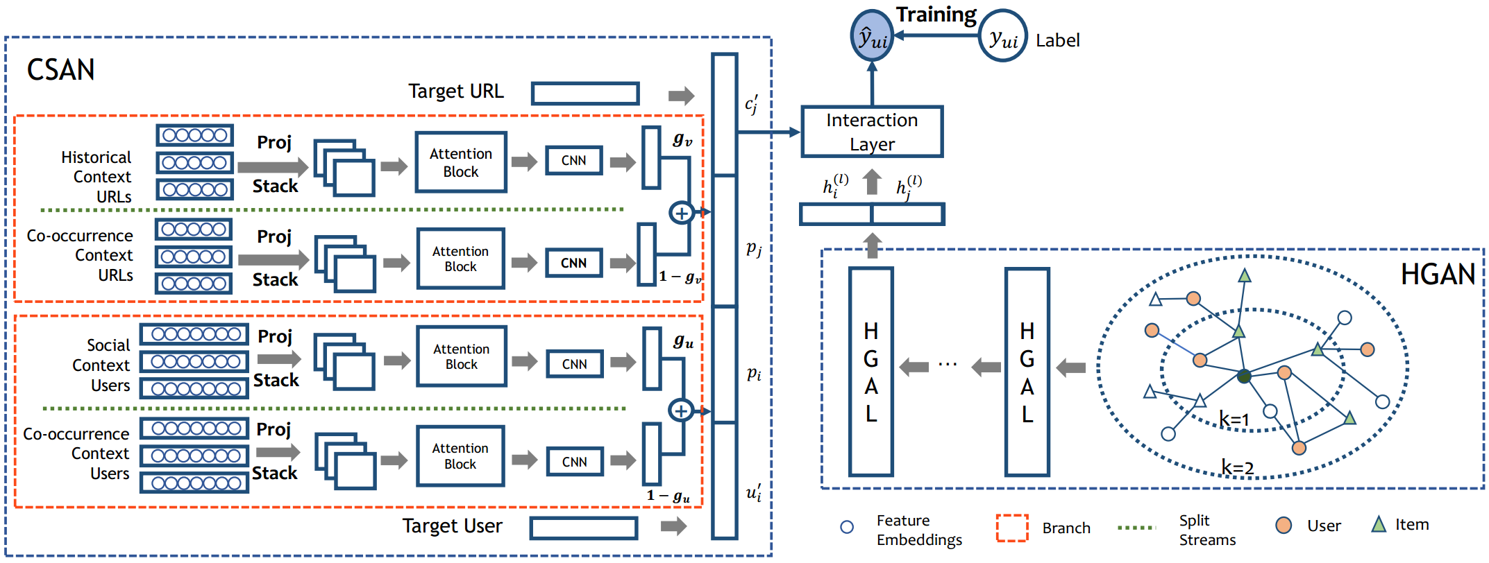
At the high level, AMRAN is composed of two modules as shown in Figure 3: (i) a convolutional spatial attention network (CSAN) and (ii) a heterogeneous graph attention network (HGAN). CSAN jointly models the influence of multi-relational context on target user-URL pair (Section 4.1). It enriches the neighborhood diversity, and expands the scope of information reception. HGAN leverages both global node connectivity and local node attributes, in order to incorporate the effect of information propagation and encode user’s dynamic preference in depth (Section 4.2). At the final step, the model produces recommendations by combining wide context-aware target user embedding and URL embedding, multi-relational context user embedding and context URL embedding, and deep context-aware user embedding and URL embedding (Section 4.3).
4.1. Convolutional Spatial Attention Network (CSAN)
The left bounding box in Figure 3 illustrates the structure of CSAN module. To provide a broad scope of knowledge for generating wide context-aware target user embedding and URL embedding, we adopt a multi-branch setting in CSAN. The two parallel branch models multi-relational context for target user and target URL respectively. Each branch contains two identical streams. We select context neighbors for each stream (e.g., historical context URL neighbors and co-occurrenced context URL neighbors of target URL, social context user neighbors and co-occurenced user neighbors of target user). These streams are employed to learn the most discriminative features from multi-relational neighbors of target user and target URL. Then we employ a gated fusion layer to capture the optimal global level representation of target user-URL pair.
Note that we enable the embedding sharing within each branch as users/URLs share the same feature set.
4.1.1. Raw Attribute Input
User and URL associate with different feature sets. Therefore, CSAN starts from embedding the input attribute set of each context neighbor. We use and to denote the number of features related to user and URL, respectively. Note that the dimension of initial embedding for each attribute could be different since they may carry with different information volume. We use one-hot encoding for categorical feature inputs, and apply direct lookup on these features. However, the same solution performs poorly when it comes continuous attributes such as the post frequency of an URL. Empirically, we found that an available solution is to bucketize these features into small intervals. Specifically, we map these continuous attributes in range into in this work.
4.1.2. Attribute Embedding Layer
We then project them into the same latent space via a set of attribute-specific transformation matrices to project all the attributes into a -dimensional space. The attributes of each neighbor then are stacked as a matrix in shape of for users and for URLs.
However, we treat the target user-URL pair differently. After projecting attributes by the same attribute-specific transformation matrix as their relational neighbors, instead of stacking them as a matrix, we concatenate the attribute embedding vectors together and feed it through a linear projection to generate and for future reference.
4.1.3. Spatial Attention Block

To prevent some unknown misalignment and conduct better comparison among the neighborhood features, we proposed a schema for jointly learning the layer-wise and channel-wise attention. In particular, for each stream, we pile the neighbors’ representation matrices together to obtain a -dimensional tensor . Intuitively, the design helps improve the alignment quality of neighbor’s features. Then, inspired by (Hu et al. 2018; Li et al. 2018), we employ a spatial attention block in each stream for jointly learning channel-level and layer-level soft attention. See figure 4 for a high-level illustration of our spatial attention block. All the streams adopt identical spatial attention blocks, and each block attends the input attribute representations independently.
In the figure, we use the historical context URL stream for illustration. The output of spatial attention block is an attention weight map which is in the same shape with the input tensor . Intuitively, the layer-wise attention and channel-wise attention are dedicated to selecting the most discriminative features and the most important neighbors, respectively. Thus, they are highly complementary to each other in functionality; and we adopt a factorized manner for optimization and computational efficiency as:
| (2) |
where and denote the layer-wise feature map and channel-wise feature map, respectively. is the result of tensor multiplication.
Layer-wise Attention
Conceptually, the layer-wise attention learns globally important elements in the feature. We apply a cross-channel average pooling operation onto the input tensor, following by 2 convolution layers of and filter, respectively. Specifically, cross-channel average pooling operation is defined as:
| (3) |
where is the number of selected neighbors.
Channel-wise Attention
The design of channel-wise attention is very similar to layer-wise attention, which aims to acquire a global view of discriminative users. Formally, the global average pooling is defined as:
| (4) |
where and are shared height and width of all channels. Similarly, we employ two convolution layers after the pooling operation.
Note that each convolution layer was followed by batch normalization operation. Furthermore, as other work of modern CNN structure (Szegedy et al. 2016), we append a ReLU activation function to assure .
We further introduce one more convolution layer of filter for enhancing the fusion of the layer-wise attention and channel-wise attention. The output tensor then is fed through a sigmoid function for normalization and generate the final attention weight tensor of spatial attention block. Formally, the output of the spatial attention module is the element-wise product of initial feature tensor and generated attention weights :
| (5) |
Intuitively, the attended feature map learned fine-grained important elements via high alignment and compatible attentions.
4.1.4. Gated Branch Fusion Layer
We apply another CNN layer of filter after the attended user representation of each stream for feature extraction and dimension :
| (6) |
| (7) |
which produces the multi-relational context representation vectors: and for each stream, respectively.
We employ a gated mechanism to assigns different weights to relation-specific neighborhood representation as:
| (8) |
| (9) |
where scalars and are learned automatically to control the importance of the two streams within each branch.
4.2. Heterogeneous Graph Attention Network (HGAN)
Following recent success in Graph Convolutional Network (GCN) (Kipf and Welling 2016; Gao et al. 2018; Schlichtkrull et al. 2018; Hamilton et al. 2017; Veličković et al. 2018). We propose a heterogeneous graph attention network (HGAN) which is tailored for recommendation task. In particular, our proposed module adopts a parallel attention structure for the user neighbor and the URL neighbor of the central node, respectively. Considering a heterogeneous graph , the nodes represent objects in this network which can be either user or URL. The edges denote the relation between connected nodes. The node attributes pass along the edges during the propagation. We try to leverage between the local node attributes and global network structure. Our novelty lies in two aspects: (i) we differentiate the contribution of URL node and user node, respectively; and (ii) we consider both similarities of node and the influence of different relation types.
While the CSAN obtains information from multi-relational immediate neighbors, which expand the scope of knowledge for target user and target URL representations, HGAN aims at learning deeper semantic representations of target user and target URL.
4.2.1. Heterogeneous Graph Network
We try to capture different semantic relation behind various types of nodes and edges. For every single layer, if the central node is user node, its neighborhood contains its co-occurrenced users and posted URLs. If the central node type is URL, its neighborhood nodes consist of users who posted it and its co-occurrenced URLs.
We adopt similar embedding approach as we did in CSAN for the initial representation of each node, but we concatenate all the features into a long vector for each node instead of stacking them as a matrix. Considering the different types of the node associated with the varied feature set, we use a set of node type-specific transformation matrices to project different types of node representation into the same feature space before aggregation as follows:
| (10) |
Let be the embedding matrix of all the attributed nodes, where is the total number of nodes and d is the dimension of latent embedding space; each row stands for the initial embedding vector of node .
We define edges based on users’ reference of URL (user-URL edges), user co-occurrence relation (user-user edges), and URL co-occurrence (URL-URL edges). We then introduce an adjacency matrix of based on the importance of each edge. In particular, to compute the weight of user-user edges and URL-URL edges, we adopt a matrix named Shifted Positive Point-wise Mutual Information (SPPMI) (Levy and Goldberg 2014), a popular measure for word associations, to utilize the co-concurrence context information. In word embedding scenario, each cell within the matrix measures the relation of corresponding word-context pair. The factorization of such matrix is proved to be equivalent to skip-gram model with negative sampling (SGNS). The Point-wise Mutual Information (PMI) between node and node is computed as where and . denotes the total number of observed word-context pairs within a predefined sliding window. is the joint probability that word and word appear together within the window size. Furthermore, we introduce the SPPMI matrix as an extension based on PMI value:
| (11) |
where is a hyperparameter, which represents the number of negative samples. Conceptually, a positive PMI value implies a semantically correlated word-context pair, Therefore, SPPMI, which only takes the positive value of PMI shifted by a global constant, reflects a closer semantic relation between word-context pairs. Inspired by this concept/idea, we use to denote the number of times of user (URL) co-occurrence and generate the user co-occurrence matrix in shape of and URL co-occurrence matrix of . Note that we do not discriminate between the target node and context node.
Similarly, we learn from the TF-IDF concept and redefine it on recommendation task with implicit feedback (Fayyad et al. 1996) as:
| (12) |
where represents the number of times URL be posted by user . further normalizes it by the maximum number of post times of any URL by user . The is associated with the user’s previous behavior as denotes the total number of URLs and is the number of URLs posted by user .
Formally, the weight of the edge between node and node is defined as:
| (13) |
4.2.2. Heterogeneous Attention Layer (HGAL)
Given the node’s initial representation defined as above, we then pass messages to aggregate the neighborhood nodes’ information and combine it with the target user’s interests. A popular propagation strategy in existing GCN works is the normalized Laplacian matrix (Kipf and Welling 2016). Even though it proves to be effective, it is not trainable and it assigns every adjacent node with the same weight. Following previous work (Veličković et al. 2018), we propose to incorporate a hierarchical attention mechanism to learn the weight of each adjacent node adaptively.
Since the distribution of the number of neighbors of each node disperses greatly, sub-sampling becomes an essential procedure in our task to avoid an explosion of computation cost after multiple hops stacked. We adopt Weighted Random Selection (WRS) (Efraimidis and Spirakis 2006) to select a fixed number of nodes for both node types in each graph attention layer. Figure 5 shows a graphical illustration of one HGAL.

Assume that the central node is a user node. We separately calculate the attention weights between the user node and its user node neighbors, or between the user node and its URL node neighbors. The similarity between the target user’s node representation and all of its selected neighbors are defined as:
| (14) |
where is the representation of user at layer , and denotes the node type-based neighbor. We adopt as similarity function. Intuitively, measures the importance of neighbor towards central node . Meanwhile, we obtain the edge weight as well.
After this, we aggregate the type-based neighborhood node representation and generate the embedding of neighborhood as the average of different types of nodes:
| (15) |
| (16) |
To model the information propagation and capture higher-order relations, we stack the HGAL multiple times. In addition, we introduce the residual connection (He et al. 2016) to help train a HGAN with many layers.
| (17) |
| (18) |
where denotes the sigmoid function. and are the shared weight matrix and bias term at layer , respectively. The node representation at -th layer provides knowledge of degrees away.
4.3. Interaction Layer
The interaction layer is tailored for recommendation tasks. Recall that we obtained wide context-based user embedding and URL embedding , context representations , and deep context-based user embedding and URL embedding in the previous sections. Then we formulate the final URL-dependent user representation by using a fully connected layer as:
| (19) |
where and are a linear transformation weight matrix and bias term, respectively. denotes vector concatenation. Note that the fully-connected layer can be replaced by other techniques (e.g. CNN). Finally, we feed it through a softmax function to calculate the probability that user interested in the given URL.
4.4. Training
We adopt the cross-entropy loss function during the training process.
| (20) |
We follow a uniform sampling strategy to obtain negative samples from unobserved interactions. Since the entire architecture is differentiable, we use back propagation to achieve end-to-end training.
5. Evaluation
In this section, we describe a dataset, baselines, experimental setting, and experimental results. In the experiments, we seek to answer the following research questions:
-
RQ1: What is the performance of our model and baselines?
-
RQ2: How beneficial is each submodule of our model?
-
RQ3: How effective is our attention mechanisms?
-
RQ4: What is sensitivity of our model with regard to hyperparameters?
5.1. Dataset
We evaluate our proposed model on a Twitter dataset obtained from the authors of (Vo and Lee 2018)22 2 https://github.com/nguyenvo09/CombatingFakeNews. The interaction behavior collected in the dataset is consistent with our definition in 3. As they did for their study, we only kept users who have at least three interactions (i.e., posting at least three fact-checking messages containing fact-checking URLs). We conducted additional preprocessing step by removing users whose posts are non-English, or their tweets were inaccessible, because some of our baselines require a fact-checker’s tweets. Our final dataset consists of 11,576 users (i.e, fact-checkers), 4,732 fact-checking URLs and 63,429 interactions. The dataset also contains each user’s social network information. Note that each user’s social relationship is restricted within available users in the dataset. And we further take available feature values of both user and URL into consideration. For instance, a category of referred fact-checking article and the name of corresponding fact-checking website reveals linguistic characteristics such as writing style and topical interest of each URL; while the number of followers and number of followees of each user indicates the credibility and influence of the fact-checker. Statistics of the final dataset is presented in Table 2.
5.2. Baselines
To measure relative effectiveness of our model, we compare our model against eight state-of-the-art baselines including the traditional collaborative filtering method, neural network-based models, and context-aware approaches.
-
MF (Koren et al. 2009) is a standard collaborative filtering technique. It factorizes an interaction matrix into two matrices and . contains each user’s latent representation, and contains each URL’s latent representation.
-
GAU (Vo and Lee 2018) is a framework specifically designed for fact-checking URL recommendation utilizing rich side information such as a user’ social network, tweets, and referred fact-checking pages. It is the most relevant and domain-specific baseline.
-
NeuMF (He et al. 2017) is a neural network based item recommendation algorithm. We adopted a composite version of MF jointly coupled with a MLP.
-
CMN (Ebesu et al. 2018) combines a global latent factor model with an augmented memory network to capture personalized neighbor-based structure in a non-linear fashion.
-
NAIS (He et al. 2018) is an item-based collaborative filtering architecture that integrates attention mechanism to distinguish the contribution of previously consumed items. The authors proposed two versions of NAIS: (1) which concatenates two vectors to learn the attention weight; and (2) which feeds the element-wise product of the two vectors to the attention network. Therefore, we also build two versions of NAIS, and compare them with our model.
-
DeepCoNN (Zheng et al. 2017) was originally proposed for an item rating prediction task which jointly model user and item based on their textual reviews. The prior work shows that it significantly outperforms other topic modeling based methods.We re-implemented the baseline and adapted it for our recommendation task with implicit feedback.
-
NARRE (Chen et al. 2018) is a deep neural network based framework for a item rating prediction task. It employs the attention mechanism to distinguish the importance of each review. We re-implemented the framework for our implicit feedback situation.
-
NGCF (Wang et al. 2019) is a new recommendation framework based on graph neural network, explicitly encoding the collaborative signal in the form of high-order connectivity in user-item bipartite graph by performing embedding propagation.
Table 3 presents characteristics of baselines and our model, showing what information each model utilizes. Note that even though CMN and NAIS both utilize co-occurrence context, CMN only utilizes user co-occurrence context whereas NAIS looks into URL co-occurrence context.
| Interaction # | User # | URLs # | Sparsity |
|---|---|---|---|
| 63429 | 11576 | 4732 | 99.884% |
| MF | GAU | NeuMF | CMN | NAIS | DeepCoNN | NARRE | NGCF | AMRAN | |
|---|---|---|---|---|---|---|---|---|---|
| Implicit Feedback | |||||||||
| Textual Content | |||||||||
| Co-occurrence Context | |||||||||
| Social Context | |||||||||
| Higher-order Information | |||||||||
| Deep Learning |
5.3. Evaluation Protocol
We adopt the leave-one-out evaluation protocol to evaluate the performance of our model and baselines. The leave-one-out evaluation protocol has been widely used in top-K recommendation tasks. In particular, we held the latest interaction of each user as the test set and used the remaining interactions for training. Each testing instance was paired with 99 randomly sampled negative instances. Each recommendation model ranks the 100 instances according to its predicted results. The ranked list is judged by Hit Ratio (HR) (Deshpande and Karypis 2004) and Normalized Discount Cumulative Gain (NDCG) (He et al. 2015) at the position 10. HR@10 is a recall-based metric, measuring the percentage of the testing item being correctly recommended in the top-10 position. NDCG@10 is a ranked evaluation metric which considers the position of the correct hit in the ranked result. Since both modules in our framework introduce randomness, we repeat each experiment 5 times with different weight initialization and randomly selecting neighbors. We report the average score of the best performance in each training process for both metrics to ensure the robustness of our framework.
5.4. Hyper-parameter Settings
We implement our framework by using Pytorch framework, initialize weight parameters by Xavier initialization (Goodfellow et al. 2016), and optimize the model with Adam optimizer (Kingma and Ba 2014). The mini-batch size is set to 128. Empirically, in CSAN, we select 10 neighbors for each stream. In HGAN, we choose 8 user neighbors and 8 URL neighbors for each central node at a single layer, and the default number of graph attention layers is set to 2. If the object (i.e.g, user neighbor or URL neighbor) is not sufficient enough, we pad the sequence with zeros vectors.
In the proposed AMRAN model, all hyperparameters are tuned by using the grid-search on the validation set, which is formed by holding out one interaction of each user from the training data like the prior work (He et al. 2017). We conduct the grid search over a latent dimension size from {8,16,32,64}, a regularization term from {0.1, 0.01, 0.001, 0.0001, 0.00001}, a learning rate from {0.0001, 0.0003, 0.001, 0.01, 0.05, 0.1}, and SPPMI shifted constant value from {1, 2, 5, 10}. The number of negative samples w.r.t each positive interaction is set to 4. We adopt the same latent dimension size for all sub-modules. For a fair comparison, we also thoroughly optimize the baselines’ hyperparameters by using the validation set.
5.5. RQ1: Performance of Our Model and Baselines
| Model | HR@10 | NDCG@10 |
|---|---|---|
| MF | 0.537 | 0.364 |
| GAU | 0.589 | 0.372 |
| NeuMF | 0.621 | 0.389 |
| CMN | 0.589 | 0.382 |
| NAIS_prod | 0.617 | 0.392 |
| NAIS_concat | 0.624 | 0.398 |
| DeepCoNN | 0.609 | 0.377 |
| NARRE | 0.615 | 0.382 |
| NGCF | 0.600 | 0.373 |
| our AMRAN | 0.657 | 0.410 |
Table 4 presents performance of our model and baselines. According to the results and information described in Table 3, we had the following observations. First, deep learning-based approaches usually obtained better performance than traditional models (e.g., MF and GAU). This observation makes sense because (1) traditional models failed to capture the important non-linear relationship between users and fact-checking URLs; (2) Most deep-learning based baseline models employ attention mechanism which helps better understand the semantic relation between user and URL; and (3) training tricks such as drop out and batch normalization also contribute to a better quality of training. In particular, achieves better performance than which supports the reason (1).
The second observation is that models with text review achieve better results compared with collaborative filtering-based methods. It is not surprising since that textual content contains rich information which could be auxiliary information to implicit feedback data and thus improve the recommendation accuracy. However, we observed that text-based recommendation approaches usually have a high complexity. Third, social context and co-occurrence context play important roles in improving recommendation results. NAIS significantly outperforms CMN and becomes the strongest baseline model. It indicates that URL-URL co-occurrence relationship is more important than user-user co-occurrence relationship since semantic representation of each user is much complex than semantic representation of a fact-checking URL.
Overall, our AMRAN outperforms all baselines, achieving 0.657 HR@10 and 0.410 NDCG@10. It improves HR@10 by 5.3% and NDCG@10 by 3% over the best baseline (i.e., ).
| Model | HR@10 | NDCG@10 |
|---|---|---|
| our CSAN | 0.642 | 0.387 |
| our HGAN | 0.653 | 0.403 |
| our AMRAN | 0.657 | 0.410 |
5.6. RQ2: Effectiveness of our submodules
In this experiment, we are interested in measuring effectiveness of our submodules of AMRAN: CSAN and HGAN. Table 5 the experimental result. CSAN achieves 0.642 HR@10 and 0.387 HR@10, whereas HGAN achieves 0.653 HR@10 and 0.403 NDCG@10. Both of the submodules outperform all the baselines in HR@10. HGAN outperforms all the baselines, and CSAN is competitive over the baselines. This experimental result confirms that both CSAN and HGAN positively contributed to the performance of our AMRAN.
5.7. RQ3: Effectiveness of our Attention Mechanisms
We proposed two attention mechanisms: (1) spatial attention block in CSAN; and (2) graph attention mechanism in HGAN described in Section 4. In this experiment, we are interested in studying the impact of the attention mechanisms. In particular, we run each submodule of AMRAN (i.e., CSAN or HGAN) with/without a corresponding attention mechanism. Table 6 shows performance of these models. In both submodules, our proposed attention mechanisms positively improved the performance of these submodules, confirming the positive impact toward correctly recommending fact-checking URLs.
| HR@10 | NDCG@10 | |
|---|---|---|
| Without Spatial Attention Block | 0.614 | 0.368 |
| CSAN | 0.642 | 0.387 |
| Without Graph Attention Mechanism | 0.638 | 0.389 |
| HGAN | 0.653 | 0.403 |
5.8. RQ4: Hyperparameter Sensitivity


Now, we turn to analyze how our model is sensitive to hyperparameter values, and which hyperparameter value produces the best recommendation result. Recall that we utilize the context information to generate comprehensive embedding of given user and URL. In CSAN, we employ four streams to capture fine-grained context characteristics and share the embedding weight matrix with the target user and target URL representations. In the first experiment, we vary the number of neighbors associated with each steam in CSAN to show how CSAN’s performance is changed. Figure 6 shows that both and have similar trends, and selecting 10 neighbors at each stream produced the best result.
Next, we measure how performance of HGAN is changed when varying the number of HGALs and a size of selected neighbor nodes at each layer. Figure 7 demonstrates the necessity of employing 2 HGALs, which consistently outperforms the one HGAL. The best performance was achieved when a size of selected neighbor nodes was set to 8. In addition, we vary the number of negative samples, and a size of latent semantic space for the target user and target URL (i.e., an embedding vector size of the target user and target URL). Figure 8 shows high dimensional latent semantic space produces high performance of AMRAN. 64 dimensional embeddings produced the best results. We also observe that one negative sample would not be enough to produce good results in especially when an embedding vector size is small. The top performance is achieved when one positive instance paired with 3 or 4 negative instances.
5.9. Case Study: Visualization of Relevance Propagation

Attention mechanism not only improve recommendation performance of our model, but also provide explainability of our model. As a case study, we specifically chose an example to demonstrate relevance propagation. In particular, we randomly sampled a user 7849 as the example as shown in Figure 9. The user 7849 has 3 co-occurrenced users, 3 following users, and posted 4 URLs. Note that we omit less important 2nd-degree neighbors for simplicity. The most relevant neighbors and the propagation paths are highlighted automatically via the attention mechanism. In general, based on the user’s historical context URLs, we observe that the topic that user 7849 would like to participate in debunking is fauxtography. However, in this very particular case, the most influential context neighbors of the user are user 25 (co-occurrence user) and user 4759 (social context) given URL 1623. Both of the context neighbors share the similar taste with user 7849 on the favorite website (Politifact.com). Moreover, we found that URL 2525 appeared in 2nd-degree neighborhood of the user 7849, and was originated from the same website (Snopes.com) with URL 1623.
6. Conclusion
In this paper, we proposed a novel framework, which effectively recommends relevant fact-checking URLs to fact-checkers. The proposed framework inspired by recent advancements in graph neural network and attention mechanism leveraged user-URL specific context information to capture deep semantic and complex structure between target user and target URL. We compared the performance of our model, AMRAN, with eight state-of-the-art baselines. Experimental results showed that our model achieved up to 5.3% improvement against the best baseline. Both submodules of AMRAN positively contributed to the recommendation results.
Acknowledgements.
This work was supported in part by NSF grant CNS-1755536, AWS Cloud Credits for Research, and Google Cloud. Any opinions, findings and conclusions or recommendations expressed in this material are the author(s) and do not necessarily reflect those of the sponsors.References
- (1)
- Allcott and Gentzkow (2017) Hunt Allcott and Matthew Gentzkow. 2017. Social media and fake news in the 2016 election. Journal of economic perspectives 31, 2 (2017), 211–36.
- Bahdanau et al. (2015) Dzmitry Bahdanau, Kyunghyun Cho, and Yoshua Bengio. 2015. Neural Machine Translation by Jointly Learning to Align and Translate. CoRR abs/1409.0473 (2015).
- Bastidas Guacho et al. (2018) Gisel Bastidas Guacho, Sara Abdali, Neil Shah, and Evangelos Papalexakis. 2018. Semi-supervised Content-Based Detection of Misinformation via Tensor Embeddings. In ASONAM.
- Chen et al. (2018) Chong Chen, Min Zhang, Yiqun Liu, and Shaoping Ma. 2018. Neural Attentional Rating Regression with Review-level Explanations. In WWW.
- Chen et al. (2017) Jingyuan Chen, Hanwang Zhang, Xiangnan He, Liqiang Nie, Wei Liu, and Tat-Seng Chua. 2017. Attentive collaborative filtering: Multimedia recommendation with item-and component-level attention. In SIGIR.
- Deshpande and Karypis (2004) Mukund Deshpande and George Karypis. 2004. Item-based top-N Recommendation Algorithms. ACM Trans. Inf. Syst. 22, 1 (Jan. 2004), 143–177.
- Ebesu et al. (2018) Travis Ebesu, Bin Shen, and Yi Fang. 2018. Collaborative Memory Network for Recommendation Systems. In SIGIR.
- Ecker et al. (2010) Ullrich KH Ecker, Stephan Lewandowsky, and David TW Tang. 2010. Explicit warnings reduce but do not eliminate the continued influence of misinformation. Memory & cognition 38, 8 (2010), 1087–1100.
- Efraimidis and Spirakis (2006) Pavlos S Efraimidis and Paul G Spirakis. 2006. Weighted random sampling with a reservoir. Inform. Process. Lett. 97, 5 (2006), 181–185.
- Fayyad et al. (1996) Usama M Fayyad, Gregory Piatetsky-Shapiro, Padhraic Smyth, and Ramasamy Uthurusamy. 1996. Advances in knowledge discovery and data mining. (1996).
- Figueira and Oliveira (2017) Álvaro Figueira and Luciana Oliveira. 2017. The current state of fake news: challenges and opportunities. Procedia Computer Science (2017).
- Gao et al. (2018) Hongyang Gao, Zhengyang Wang, and Shuiwang Ji. 2018. Large-Scale Learnable Graph Convolutional Networks. In KDD.
- Goodfellow et al. (2016) Ian Goodfellow, Yoshua Bengio, and Aaron Courville. 2016. Deep Learning. MIT Press. http://www.deeplearningbook.org.
- Hamilton et al. (2017) Will Hamilton, Zhitao Ying, and Jure Leskovec. 2017. Inductive Representation Learning on Large Graphs. In NIPS.
- He et al. (2016) Kaiming He, Xiangyu Zhang, Shaoqing Ren, and Jian Sun. 2016. Deep Residual Learning for Image Recognition. CVPR (2016).
- He and McAuley (2016) Ruining He and Julian McAuley. 2016. Ups and downs: Modeling the visual evolution of fashion trends with one-class collaborative filtering. In WWW.
- He et al. (2015) Xiangnan He, Tao Chen, Min-Yen Kan, and Xiao Chen. 2015. TriRank: Review-aware Explainable Recommendation by Modeling Aspects. In CIKM.
- He et al. (2018) Xiangnan He, Zhankui He, Jingkuan Song, Zhenguang Liu, Yu-Gang Jiang, and Tat-Seng Chua. 2018. NAIS: Neural Attentive Item Similarity Model for Recommendation. IEEE Transactions on Knowledge and Data Engineering 30 (2018), 2354–2366.
- He et al. (2017) Xiangnan He, Lizi Liao, Hanwang Zhang, Liqiang Nie, Xia Hu, and Tat-Seng Chua. 2017. Neural Collaborative Filtering. In WWW.
- Hu et al. (2018) Jie Hu, Li Shen, and Gang Sun. 2018. Squeeze-and-Excitation Networks. CVPR.
- Kalsnes (2018) Bente Kalsnes. 2018. Fake News. https://oxfordre.com/communication/view/10.1093/acrefore/9780190228613.001.0001/acrefore-9780190228613-e-809
- Kingma and Ba (2014) Diederik P Kingma and Jimmy Ba. 2014. Adam: A method for stochastic optimization. arXiv preprint arXiv:1412.6980 (2014).
- Kipf and Welling (2016) Thomas N. Kipf and Max Welling. 2016. Semi-Supervised Classification with Graph Convolutional Networks. CoRR abs/1609.02907 (2016).
- Kogan et al. (2017) Shimon Kogan, Tobias J Moskowitz, and Marina Niessner. 2017. Fake News in Financial Markets. Working Paper (2017).
- Koren et al. (2009) Yehuda Koren, Robert Bell, and Chris Volinsky. 2009. Matrix Factorization Techniques for Recommender Systems. Computer 42, 8 (Aug. 2009), 30–37.
- Levy and Goldberg (2014) Omer Levy and Yoav Goldberg. 2014. Neural Word Embedding as Implicit Matrix Factorization. In NIPS.
- Li et al. (2018) Wei Li, Xiatian Zhu, and Shaogang Gong. 2018. Harmonious attention network for person re-identification. In CVPR.
- Liu and Wu (2018) Yang Liu and Yi-Fang Brook Wu. 2018. Early detection of fake news on social media through propagation path classification with recurrent and convolutional networks. In AAAI.
- Mikolov et al. (2013) Tomas Mikolov, Ilya Sutskever, Kai Chen, Greg S Corrado, and Jeff Dean. 2013. Distributed representations of words and phrases and their compositionality. In NIPS.
- Nyhan and Reifler (2010) Brendan Nyhan and Jason Reifler. 2010. When corrections fail: The persistence of political misperceptions. Political Behavior 32, 2 (2010), 303–330.
- Quattrociocchi et al. (2016) Walter Quattrociocchi, Antonio Scala, and Cass R Sunstein. 2016. Echo chambers on Facebook. Available at SSRN 2795110 (2016).
- Sarwar et al. (2001) Badrul Sarwar, George Karypis, Joseph Konstan, and John Riedl. 2001. Item-based Collaborative Filtering Recommendation Algorithms. In WWW.
- Schlichtkrull et al. (2018) Michael Sejr Schlichtkrull, Thomas N. Kipf, Peter Bloem, Rianne van den Berg, Ivan Titov, and Max Welling. 2018. Modeling Relational Data with Graph Convolutional Networks. In ESWC.
- Seo et al. (2017) Sungyong Seo, Jing Huang, Hao Yang, and Yan Liu. 2017. Interpretable convolutional neural networks with dual local and global attention for review rating prediction. In RecSys.
- Shu et al. (2017) Kai Shu, Amy Sliva, Suhang Wang, Jiliang Tang, and Huan Liu. 2017. Fake news detection on social media: A data mining perspective. ACM SIGKDD Explorations Newsletter 19, 1 (2017), 22–36.
- Shu et al. (2019) Kai Shu, Suhang Wang, and Huan Liu. 2019. Beyond News Contents: The Role of Social Context for Fake News Detection. In WSDM.
- Silverman (2016) Craig Silverman. 2016. This analysis shows how viral fake election news stories outperformed real news on Facebook. BuzzFeed News (2016).
- Sun et al. (2011) Yizhou Sun, Jiawei Han, Xifeng Yan, Philip S Yu, and Tianyi Wu. 2011. Pathsim: Meta path-based top-k similarity search in heterogeneous information networks. Proceedings of the VLDB Endowment 4, 11 (2011), 992–1003.
- Szegedy et al. (2016) Christian Szegedy, Vincent Vanhoucke, Sergey Ioffe, Jonathon Shlens, and Zbigniew Wojna. 2016. Rethinking the Inception Architecture for Computer Vision. In CVPR.
- Tschiatschek et al. (2018) Sebastian Tschiatschek, Adish Singla, Manuel Gomez Rodriguez, Arpit Merchant, and Andreas Krause. 2018. Fake News Detection in Social Networks via Crowd Signals. In WWW.
- Van den Oord et al. (2013) Aaron Van den Oord, Sander Dieleman, and Benjamin Schrauwen. 2013. Deep content-based music recommendation. In NIPS.
- Vaswani et al. (2017) Ashish Vaswani, Noam Shazeer, Niki Parmar, Jakob Uszkoreit, Llion Jones, Aidan N Gomez, Ł ukasz Kaiser, and Illia Polosukhin. 2017. Attention is All you Need. In NIPS.
- Veličković et al. (2018) Petar Veličković, Guillem Cucurull, Arantxa Casanova, Adriana Romero, Pietro Liò, and Yoshua Bengio. 2018. Graph Attention Networks. In ICLR.
- Vo and Lee (2018) Nguyen Vo and Kyumin Lee. 2018. The Rise of Guardians: Fact-checking URL Recommendation to Combat Fake News. In The 41st International ACM SIGIR Conference on Research and Development in Information Retrieval. 275–284.
- Vo and Lee (2019) Nguyen Vo and Kyumin Lee. 2019. Learning from Fact-checkers: Analysis and Generation of Fact-checking Language. In The 42nd International ACM SIGIR Conference on Research and Development in Information Retrieval. 335–344.
- Wang et al. (2017a) Suhang Wang, Yilin Wang, Jiliang Tang, Kai Shu, Suhas Ranganath, and Huan Liu. 2017a. What your images reveal: Exploiting visual contents for point-of-interest recommendation. In WWW.
- Wang et al. (2019) Xiang Wang, Xiangnan He, Meng Wang, Fuli Feng, and Tat-Seng Chua. 2019. Neural Graph Collaborative Filtering. In SIGIR.
- Wang et al. (2017b) Xuejian Wang, Lantao Yu, Kan Ren, Guanyu Tao, Weinan Zhang, Yong Yu, and Jun Wang. 2017b. Dynamic attention deep model for article recommendation by learning human editors’ demonstration. In KDD.
- Wang et al. (2018) Yaqing Wang, Fenglong Ma, Zhiwei Jin, Ye Yuan, Guangxu Xun, Kishlay Jha, Lu Su, and Jing Gao. 2018. EANN: Event Adversarial Neural Networks for Multi-Modal Fake News Detection. In KDD.
- Wu and Liu (2018) Liang Wu and Huan Liu. 2018. Tracing fake-news footprints: Characterizing social media messages by how they propagate. In WSDM.
- Zheng et al. (2017) Lei Zheng, Vahid Noroozi, and Philip S Yu. 2017. Joint deep modeling of users and items using reviews for recommendation. In WSDM.
- Zhou et al. (2019) Xinyi Zhou, Reza Zafarani, Kai Shu, and Huan Liu. 2019. Fake News: Fundamental Theories, Detection Strategies and Challenges. In WSDM.
- Zhu et al. (2017) Yousong Zhu, Chaoyang Zhao, Jinqiao Wang, Xu Zhao, Yi Wu, and Hanqing Lu. 2017. Couplenet: Coupling global structure with local parts for object detection. In ICCV.