Multitask learning over graphs:
An Approach for Distributed, Streaming Machine LearningThanks: This work was submitted while R. Nassif was a post-doc at EPFL. She is now with the American University of Beirut, Lebanon (e-mail: roula.nassif@aub.edu.lb). S. Vlaski and A. H. Sayed are with Institute of Electrical Engineering, EPFL, Switzerland (e-mail: stefan.vlaski, ali.sayed@epfl.ch). C. Richard is with Université de Nice Sophia-Antipolis, France (cedric.richard@unice.fr). J. Chen is with Northwestern Polytechnical University, China (dr.jie.chen@ieee.org).
Abstract
The problem of learning simultaneously several related tasks has received considerable attention in several domains, especially in machine learning with the so-called multitask learning problem or learning to learn problem [1, 2]. Multitask learning is an approach to inductive transfer learning (using what is learned for one problem to assist in another problem) and helps improve generalization performance relative to learning each task separately by using the domain information contained in the training signals of related tasks as an inductive bias. Several strategies have been derived within this community under the assumption that all data are available beforehand at a fusion center. However, recent years have witnessed an increasing ability to collect data in a distributed and streaming manner. This requires the design of new strategies for learning jointly multiple tasks from streaming data over distributed (or networked) systems. This article provides an overview of multitask strategies for learning and adaptation over networks. The working hypothesis for these strategies is that agents are allowed to cooperate with each other in order to learn distinct, though related tasks. The article shows how cooperation steers the network limiting point and how different cooperation rules allow to promote different task relatedness models. It also explains how and when cooperation over multitask networks outperforms non-cooperative strategies.
I Multitask network models

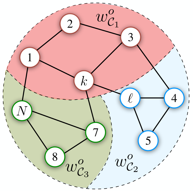

Consider a networked system consisting of a collection of autonomous agents (sensors, classifiers, etc.) distributed over some geographic area and connected through a topology. The neighborhood of agent is denoted by ; it consists of all agents that are connected to by an edge–see Fig. 1 (left). A real-valued strongly convex and differentiable cost is associated with each agent . The objective (or the task) at agent is to estimate the parameter vector, , of size , that minimizes , namely,
| (1) |
Depending on how the minimizers across the agents relate to each other, we distinguish between three categories of networks:
- 1.
Single-task network: All costs are minimized at the same location , namely, for all – see Fig. 1 (left).
- 2.
Clustered multitask network: The agents are grouped into clusters () and, within each cluster , all the costs are minimized at the same location , namely, for all – see Fig. 1 (middle). Similarities or relationships may exist among the distinct minimizers .
- 3.
Multitask network: The individual costs are minimized at distinct, though related, locations – see Fig. 1 (right).
Each agent can solve (1) on its own. However, since the objectives across the network relate to each other, it is expected that by properly promoting these relationships, one may improve the network performance. In other words, it is expected that through cooperation among the agents, one may improve the network performance. One important question is how to design cooperative strategies that can lead to better performance than non-cooperative ones where each agent attempts to determine on its own. This overview paper explains how multitask learning over graphs addresses this question.
Prior to multitask learning over graphs, there have been many works in the machine learning literature where learning multiple related tasks simultaneously has been considered [1, 2, 3, 4, 5, 6, 7]. Multitask learning was shown, both empirically and theoretically, to improve performance relative to the traditional approach of learning each task separately. Depending on the machine learning application, several task relatedness models have been considered. For example, in [1, 5], the functions to be learned are assumed to share a common underlying representation. In [6], it is assumed that the tasks are close to each other in some Hilbert space. Probabilistic based approaches, where a probability model capturing the relations between tasks is estimated simultaneously with functions corresponding to each task, have also been considered [3]. Also, graph-based approaches, where the relations between tasks are captured by an underlying graph, were also considered in the literature [4, 7]. All these works, however, assume that all data are available beforehand at a fusion center and propose batch-mode methods to solve multitask problems. Other existing works, such as [8], consider distributed data setting. However, most of these works still require an architecture consisting of workers along with a master, where agents perform local computations followed by sending intermediate results to the master for further processing. Such solution methods are not fully distributed, which limits their range of practical applications.
This paper, however, focuses on fully distributed solutions that avoid the need for central data aggregation or processing and instead rely on local computations and communication exchanges among neighborhoods. Besides providing distributed implementations, the solutions considered in this paper are able to learn continuously from streaming data. We start our exposition by describing a class of non-cooperative solutions that are able to respond in real time to streaming data. Then, we explain how these solutions can be extended to handle multitask learning over graphs.
II Noncooperative learning under streaming data
Throughout this article, there is an explicit assumption that agents operate in the streaming data setting. That is, it is assumed that each agent receives at each time instant one instantaneous realization of a random data . The goal of agent is to estimate the vector that minimizes its risk function , defined in terms of some loss function . The expectation is computed over the distribution of the data . Agent is particularly interested in solving the problem in the stochastic setting when the distribution of the data is generally unknown. This means that the risks and their gradients are unknown. As such, approximate gradient vectors will need to be employed. Doing so leads to the following stochastic gradient algorithm for solving (1):
| (2) |
where is the estimate of at iteration and is a small step-size parameter. Resorting to the instantaneous realization of the random data , a common construction in the stochastic approximation theory is to employ the following gradient approximation at iteration :
| (3) |
We therefore focus in this paper on stochastic gradient algorithms, which are powerful iterative procedures for solving (1) in the streaming data. They enable continuous learning and adaptation in response to drifts in the location of the minimizers due to changes in the costs. We illustrate construction (2)–(3) by considering scenarios from machine learning and adaptive filter theory.
Example 1.
(Logistic regression network). Let be a streaming sequence of (class) binary random variables and let be the corresponding streaming sequence of real random (feature) vectors with . The processes are assumed to be wide-sense stationary. In these problems, agent seeks to estimate the vector that minimizes the regularized logistic risk function [9]:
| (4) |
where is a regularization parameter. Once is found, can then be used as a decision rule to classify new features. Using approximation (3), we obtain the following stochastic-gradient algorithm for minimizing (4):
| (5) |
∎
Example 2.
(Mean-square-error (MSE) network). In such networks, each agent is subjected to streaming data that are assumed to satisfy a linear regression model:
| (6) |
for some unknown vector to be estimated by agent with denoting a zero-mean measurement noise. For these networks, the risk function takes the form of an MSE cost [10]:
| (7) |
which is minimized at . The processes are zero-mean jointly wide-sense stationary with: i) if and zero otherwise; if and zero otherwise; and iii) and are independent of each other. Using approximation (3), we obtain the following stochastic-gradient algorithm:
| (8) |
which is the well-known least-mean-squares (LMS) algorithm [11].∎
The use of the approximate gradient instead of the true gradient in (2) introduces perturbations into the operation of the gradient descent iteration. This perturbation is referred to as the gradient noise defined as The presence of this perturbation prevents the stochastic iterate from converging almost surely to the minimizer when constant step-sizes are used. Some deterioration in performance will occur, and the iterate will instead fluctuate close to . It is common in adaptive filtering and stochastic gradient optimization literatures to assess the size of these fluctuations by measuring their steady-state mean-square value [11, 10, 9]. We therefore focus in this paper on highlighting the benefit of multitask learning on the network mean-square-deviation (MSD), which is defined as the steady-state average variance value:
| (9) |
In the sequel, when discussing theoretical performance results, and to avoid excessive technicalities, it is sufficient to focus on MSE networks described in Example 2 and to assume that and for all 11 1 Performance results under more general conditions, such as allowing for space dependent covariances and lengths and for general second-order differentiable cost functions that are not necessarily quadratic, can also be found in [9, Chap. 3–4] for algorithm (2), in [12] for the strategy introduced in Sec. IV-A, and in [32] for the strategies in Sec. V. The MSD performance expressions in these works are derived under Lipschitz gradient vectors and Hessian matrices assumptions. It should be noted that the analyses in these works allow also to recover the Excess-Risk metric at agent , which is defined as –see, e.g., [9, p. 388–390]. Due to space limitations, we shall only focus on presenting MSD performance expressions.. In this way, the quality of the measurements, captured by the noise power , is allowed to vary across the network with some agents collecting noisier data than other agents. Assuming uniform regressors covariance allows us to quantify the improvement in performance that results from cooperation without biasing the results by the statistical nature of the regression data at the agents.
Performance result 1.
where the superscript “nc” is used to indicate that the MSD expression is for the non-cooperative solution. First, observe that the performance is on the order of . The smaller is, the better the performance will be, but the slower the convergence toward will be [9, 10] (the same observation is valid for future expressions (17) and (34) with convergence to in (17) instead). Second, observe that agents with noisier data will perform worse than agents with cleaner data. However, since agents are observing data arising from similar or related models , it is expected that an appropriate cooperation among agents can help enhance the network performance.
III Multitask learning framework
Depending on the application, several task relatedness models can be considered. For each model, an appropriate convex optimization problem is solved in a distributed and adaptive manner. This results in different multitask strategies, and therefore different cooperation rules between agents. Rather than describing each optimization problem in isolation, we begin by introducing a general problem, which will allow us to recover various multitask strategies as special cases.
Let denote the collection of parameter vectors from across the network. We consider the following global optimization problem for the multitask formulation:
| (11) |
where is a convex regularization function promoting the relationships between the tasks, is a closed convex set defining the feasible region of the parameter vectors, and is a parameter controlling the importance of the regularization. The choice of the regularizer and the set depends on the prior information on how the multitask models relate to each other. To illustrate how problem formulation (11) can be used, we consider the following two examples that are multitask oriented.


Example 3.
(Weather forecasting [12]). Consider the network in Fig. 2 (left) consisting of weather stations located across the United States and collecting daily measurements. Let denote the feature vector consisting of collected data (temperature, wind speed, dew point, etc.) at sensor and day and let denote the corresponding binary variable associated with rain occurrence, i.e., if rain occurred and otherwise. The objective is to construct a classifier at each station to predict whether it will rain or not based on the knowledge of . To this end, each station can use an individual logistic regression machine similar to the one described in Example 1; in this case the cost in (11) takes the form (4). However, it is expected that the decision rules at neighboring stations would be similar since they are collecting features arising from similar statistical distributions. Moreover, the strength of similarity is expected to be inversely proportional to the physical distance between the stations. This gives rise to a weighted graph (with closest nodes connected by edges) and one may expect to improve the network performance by promoting the smoothness of with respect to the underlying graph. The simplest possible term that encourages smoothness is the graph Laplacian regularizer defined further ahead in (13). By choosing and in (11), one arrives at a multitask formulation for the weather forecasting application that takes into account the smoothness prior over the graph. This formulation and other possible formulations are solved in Sections IV and V. ∎
Example 4.
(Power system state monitoring [13]). Consider Fig. 2 (right) illustrating an IEEE 14-bus power monitoring system partitioned into 4 areas, where each area comprises a subset of buses supervised by its own control center. The local state vectors (bus voltages) to be estimated at neighboring areas may partially overlap as the areas are interconnected. This is because each control center collects measurements related to the voltages across its local buses and voltages across the interconnection between neighboring centers. For example, Area 2 supervises buses 3, 4, 7, and 8. Since it collects current readings on lines (4, 5) and (7, 9), its state vector extends to buses 5 (supervised by Area 1) and 9 (supervised by Area 4). In other words, if we let denote the state of bus , then the cost at Area 2 will depend on the extended parameter vector . However, since the parameter vectors at Areas 1 and 4 will be and , respectively, consensus needs to be reached on the variable between Areas 2 and 1, and on the variable between Areas 2 and 4, while minimizing the individual cost penalizing deviation from data models of the form where is the measurement matrix and is a zero-mean noise. Thus, distributed power state estimation can be formulated as problem (11) with , whereas the constraint set in this case should be selected to promote consensus over the overlapped variables. In Section V-B, we explain how such problems can be solved. ∎
Returning to the formulation (11), observe that even though the aggregate cost is separable in , the cooperation between agents is necessary due to the coupling between the tasks through the regularization and the constraint. Note that, when solving problem (11), agent will be responsible for estimating (the -th sub-vector of ), which is generally different from in (1), the actual objective at agent . However, it is expected that accurate prior information will allow the designer to choose the regularizer , the set , and the strength in a way that minimizes the distance between and .

Although some existing works use primal-dual methods [14] to solve multitask estimation problems, we limit our exposition to the class of primal techniques (based on propagating and estimating the primal variable) that employ stochastic-gradient iterations. Extensive studies in the literature have shown that small step-sizes enable these strategies to learn well in streaming data settings. Due to the separability property of , the multitask algorithms described in the sequel will have a common structure given by:
| (12a) | ||||
| (12b) | ||||
The first step (12a) corresponds to the stochastic gradient step on the individual cost . We refer to this step as the self-learning step–see Fig. 3. Compared with the non-cooperative strategy (2), observe now that the result of the gradient descent step is , an intermediate estimate of at iteration . This step is followed by a social learning step (12b), which uses some function of the neighborhood iterates. As we shall see in the next sections, the form of this function depends on the regularizer and the set in (11), both of which allow to promote the prior information on how the tasks are related. The result of this second step is , the estimate of , defined by (1), at iteration . Since we are interested in a distributed setting, agents during social learning are only allowed to collect estimators from their local neighborhood –see Fig. 3.
IV Regularized multitask estimation
In this section, we focus on the regularization term in (11) and its implications for the learning dynamics. In multitask learning (MTL), regularization is a widely used technique to promote task relationships. In most network applications, the underlying graph structure contains information about the relatedness among neighboring tasks. As such, when considering graph-based MTL applications, incorporating the graph structure into the regularization term is a reasonable and natural step. The smoothness model (under which the tasks are similar at neighboring vertices with the strength of similarity specified by the weight between them) will play a central role in our discussion. This smoothness property is often observed in real world applications (see, e.g., Example 3) and is rich enough to convey the main ideas behind MTL, as we will see in the sequel. We will examine two main questions: 1) How to incorporate graph-based priors into the regularizer? and 2) How does the resulting MTL algorithm behave?
IV-A Multitask estimation under smoothness
We assume that a symmetric, weighted adjacency matrix is associated with the connected graph illustrated in Fig. 1 (right). If there is an edge connecting agents and , then reflects the strength of the relation between and ; otherwise, . These weights are usually dictated by the physics of the problem at hand–see, e.g., [15],[16, Ch. 4] for graph construction methods. We introduce the graph Laplacian , which is a differential operator defined as . Assuming that the tasks have the same length, i.e., , the smoothness of over the graph is measured in terms of a quadratic form of the Laplacian [17]:
| (13) |
where is an extended form of the graph Laplacian (defined in terms of the Kronecker product operator ). The smaller is, the smoother the signal on the graph is. Given that the weights are nonnegative, shows that is smooth if nodes with a large on the edge connecting them have similar weight values . Therefore, in order to enforce the prior belief that the target signal is smooth with respect to the underlying weighted graph, one may choose in (11):
| (14) |
Under this choice, the stochastic gradient algorithm for solving (11) takes the following form:
| (15) |
where is the estimate of at instant , and is the vector collecting the intermediate estimates in (12a) from across all agents. Since we expect to be an improved estimate compared to , we propose to replace in (15) by . By doing so, we obtain algorithm (12) with the social learning step given by:
| (16) |
The substitution of by is reminiscent of incremental-type arguments in gradient descent algorithms [18]. Analyses in the context of adaptation over networks show that substitutions of this type lead to enhanced network stability since they allow to preserve the stability of the agents after cooperation (see, e.g., [10, p. 160] for details). Regarding algorithm (16), it follows that, when the spectral radius of the combination matrix is equal to one, sufficiently small step-sizes ensuring the individual agents stability will also ensure the network stability22 2 In this article, a network is said to be stable if the mean-square-error converges asymptotically to a bounded region of the order of the step-size. [12].
IV-B Bias-variance tradeoff
We next consider the interesting question whether multitask learning is beneficial compared to noncooperation. The answer to this inquiry requires i) studying the performance of algorithm (12) relative to the actual agents objectives and then ii) examining when the multitask implementation (12) can lead to enhanced performance in comparison to the non-cooperative solution (2).
Algorithm (12) was studied in detail in [12]. It was shown that the network MSD defined by (9) is mainly influenced by the sum of two factors, as explained further below. The first factor is the steady-state variance of algorithm (12) with respect to the regularized solution in (11), namely, . The second one is the bias or the average distance between the regularized solution and the unregularized one , namely, . By increasing the regularization strength , the variance term is more likely to decrease while the bias term is more likely to increase. Understanding this bias-variance tradeoff is critical for understanding the behavior of regularized multitask algorithms.
We therefore describe in the following the bias-variance behavior of algorithm (16) by considering the expressions derived in [12]. These expressions are useful for illustrating the concept of multitask learning. As we will see, instead of involving the vertex domain given by the entries of the adjacency matrix, these expressions involve the graph spectral information defined by the eigendecomposition of the Laplacian . Because the Laplacian is a real symmetric matrix, it possesses a complete set of orthonormal eigenvectors. We denote them by . For convenience, we order the set of real, non-negative eigenvalues of as , where, since the network is connected, there is only one zero eigenvalue with corresponding eigenvector [20]. Therefore, the Laplacian can be decomposed as where and .
Performance result 2.
Consider an MSE network running the multitask algorithm (12) with the second step given by (16). Assume further that and that . Under these assumptions and for sufficiently small step-sizes and smooth signal , it is shown that [12]:
| (17) |
where
| (18) |
with the -th eigenvalue of and the -th entry of the eigenvector . For the bias term, it can be shown that [12]:
| (19) |
where
| (20) |
with the -th subvector of corresponding to the eigenvalue .∎
For the steady-state variance (17), observe that it consists of the summation of terms , each one corresponding to an eigenvalue of the Laplacian. The first one is independent of the regularization strength . The remaining terms decrease when increases. Therefore, when increases, the variance decreases. From expression (19), we observe that the bias tends to increase by increasing the regularization strength . However, an interesting fact arises for smooth . To see this, we rewrite the regularizer in (13) as:
| (21) |
where we used the fact that . Intuitively, given that for , the above expression shows that is considered to be smooth over the graph if corresponding to large eigenvalue is very small. That is, a smooth is mainly contained in , i.e., if , and the smoother is, the smaller will be. In this case, the effective sum in (19) is over the first terms (corresponding to small eigenvalues ) instead of terms. We thus conclude that as long as is sufficiently smooth, moderate regularization strengths in the range exist such that the decrease in variance at these values of will dominate the increase in bias. In other words, the MSD at these values of will be less than the MSD at , which corresponds to the noncooperative mode of operation.
Observe from (16) that the social learning step following from the Laplacian regularization term (13) involves a single communication step at every stochastic gradient update. When multiple steps are allowed, it is reasonable to expect that performance can be improved. In the following, we show how such solution can be designed.
IV-C Graph spectral regularization
The main observation behind the introduction of this regularizer is that a smooth over a graph exhibits a special structure in the graph spectral domain (it is mainly contained in , i.e., if ) [21]. Graph spectral regularization is used to leverage more thoroughly the spectral information and improve the multitask network performance. In this case, the network will aim at solving problem (11) with and properly selected in order to promote the prior information available on the structure of in the graph spectral domain. The following class of regularization functionals on graphs can be used for this purpose [21, 22]:
| (22) |
where is some well-defined non-negative function on the spectrum of and is the corresponding matrix function defined as [23, p. 3]:
| (23) |
Construction (22) uses the Laplacian as a means to design regularization operators. Requiring a positive semi-definite regularizer imposes the constraint for all . Replacing (23) into (22), we obtain – compare with the regularizer in (21) to see how an extra degree of freedom is introduced in the multitask network design:
| (24) |
where and . The regularization in (24) promotes a particular structure in the graph spectral domain. It strongly penalizes for which the corresponding is large. Thus, one prefers to be large for those that are small and vice versa. From the discussion following (21), it is clear that, under smoothness, the function must be chosen to be monotonically increasing in . One typical choice is with . Example 5 further ahead illustrates for instance the benefit of using instead of .
Assuming the regularizer in (22) can be written as an -th degree polynomial of the Laplacian , i.e., for some constants (or, equivalently, ), and following similar arguments that led to (16), one arrives at the following social step (12b) [22]:
| (25) |
where . It requires communication steps. The resulting algorithm (25) is distributed since at each step, each agent is only required to exchange information locally with its neighbors. Since communication steps are required, agent ends up collecting information from its -hop neighborhood.
For more general that are not necessarily polynomial in , one would like to benefit from the sparsity of the graph captured by . As long as can be approximated by some lower order polynomial in , say , distributed implementations of the form (25) are possible–see [22]. Problems of this type have already been considered in graph filters design [24, 25]. For instance, the work [24] proposes to locally approximate by a polynomial computed by truncating a shifted Chebyshev series expansion of on . When the regularizer is continuous, the Chebyshev approximation converges to it rapidly as increases. When the regularizer presents some discontinuities, polynomial approximation methods are not advised over adaptive networks since accurate approximation would require a large order , and consequently, a large number of communication steps at each iteration. Projection based methods similar to the one described in Sec. V can be useful in this case. For example, if the smooth signal is only contained in , instead of using a discontinuous regularizer of the form if and otherwise, one may design a multitask network that is able to project onto the space spanned by the first eigenvectors of the graph Laplacian.
Since the optimization problems in Sec. IV-A and IV-C are the same with in (13) replaced by in (22), the multitask strategy (25) will behave in a similar manner as (16). Particularly, the bias-variance tradeoff discussion continues to apply, and expressions (17)–(20) continue to hold with on the RHS of (18) and (20) replaced by the function . By replacing on the RHS of (20) by , one may directly observe the consequence of this regularizer on the bias term (19), which can be made now close to zero (by choosing in the smoothness case, for example, if and otherwise).

Example 5.
(Graph spectral filtering). Consider the MSE network example in Fig. 4 and assume uniform data profile, i.e., and . In the left plot, we illustrate the entries of the tasks , which are smooth over the underlying graph. In the middle plot, we illustrate the behavior of the previously described algorithms in the graph spectral domain. The top plot represents the behavior of the network output for three different choices of regularizer . The bottom plot represents the behavior of the steady-state variance (18) with the eigenvalue replaced by the function . Observe how the regularizer penalizes low-eigenvalues less than , and consequently preserves all the signal components . Observe further the graph low-pass filtering behavior [25, 24]. Small eigenvalues correspond to low frequencies, corresponds to the graph Fourier transform, and corresponds to the -th frequency content of . It can be shown that the -th frequency content of the output can be bounded as in terms of the -th frequency content of the input where is the maximum eigenvalue of (see [12]). Since is monotonically increasing in , for fixed , as increases, the ratio decreases. Therefore, the network output can be interpreted as the output of a low-pass graph filter applied to the signal . A similar behavior arises for the steady-state variance. For fixed , as increases, the variance at the -th frequency, i.e., , decreases, and for fixed , as increases, decreases. The regularizer controls the shape of the filter and the strength controls the sharpness. The non-cooperative solution () corresponds to an all-pass graph filter. In the right plot, we illustrate the bias-variance tradeoff in the case of .∎
Returning to the diagram in Fig. 3, observe that the self-learning step corresponds to the inference step where agent estimates from streaming data and that the social-learning step corresponds to the graph filtering step where the agents collaborate in order to perform spatial filtering and reduce the effect of the noise on the network MSD defined by (9). These steps are performed simultaneously. Therefore, multitask learning over networks allows to blend real-time adaptation with graph (spatial) filtering.
IV-D Non-quadratic regularization
Non-quadratic regularization has been also considered in the literature [26, 27, 14]. This scenario will induce non-linearities in the social learning step (12b). In this case, multitask algorithms are derived in order to solve problem (11) with
| (26) |
where is a convex cost function associated with the link . In general, this function is used to enforce some constraints on the pairs of variables across an edge. Observe that (26), by allowing arbitrary distance measures , is a generalization of the previously employed quadratic regularization. In fact, setting recovers (13). Examples of other typical choices are the -norm regularizer and the -norm regularizer . Instead of encouraging global smoothness, these sparsity-based regularizers can adapt to heterogeneity in the level of smoothness of the tasks across nodes [28]. Such heterogeneity is observed for instance in the problem of predicting housing prices [27]. In this problem, the objective at each node (house) in a graph (where neighboring houses are connected by edges) is to learn the weights of a regression model (examples of features are number of bedrooms, square footage, etc.) to estimate the price. Due to location-based factors (such as distance to highway) that are often unknown a priori and, therefore, cannot be incorporated as features, similar houses in different, though close (neighbors), locations can have drastically different prices, i.e., drastically different . The objective in this case is to encourage neighboring houses that share common models to cooperate without being influenced by the misleading information of neighbors sharing different models, i.e., perform automatic clustering. To do so, the authors in [27] propose to solve the network Lasso problem, i.e., problem (11) with -norm regularizer in (26). The rationale behind this choice is that -norm encourages group sparsity, i.e., consensus across an edge . On the other hand, the -norm regularizer is used in [26] to promote the prior that the parameter vectors at neighboring nodes have a large number of similar entries and a small number of distinct entries. The weight in (26) associated with the link aims at locally adjusting the regularization strength. It is usually dictated by the physics of the problem at hand. For primal adaptive techniques and due to the non-differentiability of the regularizers, proximal gradient methods can be used to solve (11). Assuming and , one may arrive to a multitask algorithm of the form (12) with the social learning step (12b) given by (see the derivations in [26]):
| (27) |
where denotes the proximal operator of the function :
| (28) |
and where the function is given by Notice that the proximal operator in (27) needs to be evaluated at each iteration. For the weighted sum of -regularizer, a closed form expression can be found in [26].
V Multitask estimation under subspace constraints
Besides regularized-based algorithms, projection-based algorithms have received considerable attention in the literature of deterministic [29, 30, 31, 18] and stochastic [10, 9, 32, 33, 34, 35] optimization. The objective in this case is to design distributed networks that are able to project onto low-dimensional subspaces while minimizing the individual costs, i.e., solve problems of the form (11) with [32, 29]:
| (29) |
where denotes the range space operator and is an full-column rank matrix with and . The reader will soon realize that consensus-type problems are instances of this formulation. Also, multitask estimation under smoothness can benefit from this formulation: as explained earlier in Sec. IV-C, when the first eigenvectors of the Laplacian are available, the designer can project onto with instead of using regularization.
Let denote the projection onto the range space of . Assuming that the network topology and the signal subspace are such that the following feasibility problem:
| (30) |
admits at least one solution, one may arrive to a multitask strategy of the form (12) with the social learning step (12b) given by [32]:
| (31) |
where is the -th block (of size ) of the block matrix . A matrix satisfying the constraints in (30) is semi-convergent [32, 29]. Particularly, it holds that:
| (32) |
The first two constraints in (30) state that the columns of are right and left eigenvectors of associated with the eigenvalue . Together with these two constraints, the third constraint in (30) ensures that has eigenvalues at one, and that all other eigenvalues are strictly less than one in magnitude. The last constraint in (30) corresponds to the sparsity constraint which characterizes the network topology and ensures local exchange of information at each instant .
Before explaining how some typical choices of lead to well-studied distributed inference problems, we note that the distributed algorithm (31) has an attractive property: in the small step-size regime, the iterates generated by (31) achieve the steady-state performance of the following gradient projection algorithm [32]:
| (33) |
which is centralized since, at each instant , agent needs to send its estimate in (12a) to a fusion center, which performs the projection, and then sends the result back to the agent.
Performance result 3.
Consider an MSE network running algorithm (12) with the social step (12b) given by (31) with satisfying the constraints in (30). Assume that the network is seeking . Assume further that where is semi-orthogonal, and that and for all . Under these assumptions, and for sufficiently small step-sizes, the network MSD defined by (9) is given by [32]:
| (34) |
Notice that the projection framework will not induce bias in the estimation. This is because , and, therefore, the vector in (11) is equal to , the network objective. Moreover, the benefit of cooperation can be readily seen by assuming uniform variances for all . In this case, comparing (34) with (10) in the non-cooperative case, we conclude that where . Therefore, the cooperative strategy outperforms the non-cooperative one by a factor of .
V-A Single-task estimation
In single-task estimation, the agents are seeking a common minimizer –see Fig. 1 (left). This problem is encountered in many applications. Examples include target localization and distributed sensing (see, e.g., [10]). Single-task estimation can be recast in the form (11) where and are chosen according to (29) with . Several algorithms for solving such consensus-type problems have been proposed in the literature, including incremental [18], consensus [30], and diffusion[10, 9] strategies. Due to lack of space, we will describe only the class of diffusion strategies, which can be written in the form (12) with the social step (12b) given by:
| (35) |
where corresponds to the -th entry of an doubly-stochastic matrix satisfying:
| (36) |
Several rules for selecting locally these combination coefficients have been proposed in the literature, such as the Metropolis rule and Laplacian rule; see, e.g., [9]. Observe that step (35) can be written in the form of (31) with and , and that the resulting matrix will satisfy the constraints in (30) over a strongly connected network.
V-B Multitask estimation with overlapping parameter vectors
It is assumed that the individual costs depend only on a subset of the components of a global parameter vector [31, 33, 34, 35]. This situation is observed in Example 4 where the network global parameter vector is and where the states to be estimated at neighboring areas partially overlap. It can be verified that this problem can also be recast in the form (29) with properly selected. To solve this consensus-type problem, and motivated by the single-task diffusion strategies, the works [33, 34] propose the following algorithm. Assume agent is interested in estimating the entry of and let denote the set of neighbors of that are interested also in estimating . In order to reach consensus on , agent assigns to its entry a set of non-negative coefficients satisfying
| (37) |
and performs the following convex combination:
| (38) |
where is the entry of the intermediate estimate (obtained from (12a)) corresponding to the variable and is the estimate of at node and instant . It can also be verified that solution (38) can be written in the form (31) with the block properly selected.
For MSE networks, a recursive least-squares (RLS) approach is proposed in [35] to solve overlapping multitask estimation. In general, second-order gradient methods enjoy faster convergence rates than first-order methods at the expense of increasing the computational complexity.
VI Clustered multitask estimation
Now we move into explaining how clustered multitask estimation can be solved. Clustered multitask learning was first considered in [6] within the machine learning community. Then, it was extended to adaptation and learning over networks in the work [36]. As we shall see, clustered multitask estimation merges subspace constraints with regularization. Let for all . In clustered multitask networks, agents within a cluster are interested in estimating the same vector – see Fig. 1 (middle). Without loss of generality, we index agents according to their cluster indexes such that agents from the same cluster will have consecutive indexes. Let denote the number of agents in cluster . Since agents within need to reach a consensus on , clustered multitask estimation problems can be recast in the form (11) with:
| (39) |
Therefore, the cluster consensus step takes the form (31) with and where the blocks are chosen according to the constraints in (30); one typical choice is doubly-stochastic blocks. The resulting matrix will satisfy:
| (40) |
where denotes the neighboring nodes of that are inside its cluster. The choice of the regularizer in (11) depends on the prior information on how the models across the clusters relate to each other. One typical choice is [36, 26]:
| (41) |
where denotes neighboring nodes of that are outside its cluster and is a cost associated with the inter-cluster link . This function is used to enforce some constraints on the pairs of variables across an inter-cluster edge. Examples are to enforce graph smoothness [36] and to enforce sparsity priors [26].
Clustered multitask algorithms have in general the structure (12) with step (12b) given by:
| (42a) | ||||
| (42b) | ||||
In this algorithm, the self-learning step (12a) is followed by an intra-cluster social learning step (42a) where node receives the intermediate estimates from its intra-cluster neighbors and combines them in a convex manner through the coefficients in (40) to obtain the intermediate value . The second step (42b) is an inter-cluster social learning step where agent receives the intermediate estimates from its neighbors that are outside its cluster and combines them properly using the function to obtain . This step helps to incorporate the available prior information on how the models across the clusters are related into the adaptation mechanism. The function depends on the regularizer . For example, for -norm co-regularizers (with ), one may arrive to an inter-cluster learning step (42b) given by with [26].
VII Conclusion
In this article, we explained how prior knowledge about tasks relationships can be incorporated into the adaptation mechanism and how different priors yield different multitask strategies. It then follows that choosing the optimal strategy for a given problem is equivalent to choosing the task relatedness model which best fits the underlying problem. Choosing the most practically viable solution then balances further this model fit against computational and communication constraints.
There are several other aspects and strategies for multitask learning over graphs that were not covered in this article due to space limitations. For instance, we only focused on multitask networks endowed with parameter estimation tasks. However, distributed detection was also considered from a multitask perspective (see, e.g., [37]). Online network clustering was also considered. The objective in this case is to design diffusion networks that are able to adapt their combination coefficients in (35) in order to exclude harmful neighbors sharing distinct tasks [38, 39]. Readers can refer to [40] to have a list of other literature works that are multitask oriented.
Multitask learning over graphs is worth exploring further, as there are many potential ideas to build on. For instance, the expressions show the sensitivity of the results to the underlying graph structure. It would be useful to infer the entries of the adjacency matrix in (16) simultaneously with the self-learning step (12a). This leads to learning the relations between the tasks simultaneously with the tasks. Automatically determining the optimal regularization strength and allowing edge regularizers beyond just the -norm constitute also clear extensions. Finally, we believe that the number of multitask learning applications in “distributed, streaming machine learning” is vast, and hope to witness increased utilization of the algorithms and theoretical results established in the domain of “learning and adaptation over networks”.
References
- [1] R. Caruana, “Multitask learning,” Machine Learning, vol. 28, no. 1, pp. 41–75, Jul. 1997.
- [2] S. Thrun and L. Pratt, Learning to Learn, Kluwer Academic Publishers, Norwell, MA, USA, 1998.
- [3] Y. Zhang and D. Yeung, “A convex formulation for learning task relationships in multi-task learning,” in Proc. 26th Conf. on Uncertainty in Artificial Intelligence, Catalina Island, California, U.S.A., Jul. 2010, pp. 733–742.
- [4] X. Chen, S. Kim, Q. Lin, J. G. Carbonell, and E. P. Xing, “Graph-structured multitask regression and an efficient optimization method for general fused Lasso,” Available as arXiv:1005.3579, May 2010.
- [5] T. Evgeniou and M. Pontil, “Regularized multi–task learning,” in Proc. 10th ACM SIGKDD Int. Conf. on Knowledge Discovery and Data Mining, New York, U.S.A, 2004, pp. 109–117.
- [6] L. Jacob, F. Bach, and J.-P. Vert, “Clustered multi-task learning: A convex formulation,” in Proc. 21st Int. Conf. on Neural Information Processing Systems, Vancouver, Canada, 2008, pp. 745–752.
- [7] T. Kato, H. Kashima, M. Sugiyama, and K. Asai, “Multi-task learning via conic programming,” in Proc. 20th Int. Conf. on Neural Information Processing Systems, Vancouver, Canada, 2007, pp. 737–744.
- [8] J. Wang, M. Kolar, and N. Srebro, “Distributed multi-task learning,” in Proc. Conf. on Artificial Intelligence and Statistics, Cadiz, Spain, 2016.
- [9] A. H. Sayed, “Adaptation, learning, and optimization over networks,” Foundations and Trends in Machine Learning, vol. 7, no. 4-5, pp. 311–801, 2014.
- [10] A. H. Sayed, S.-Y. Tu, J. Chen, X. Zhao, and Z. J. Towfic, “Diffusion strategies for adaptation and learning over networks,” IEEE Sig. Process. Mag., vol. 30, no. 3, pp. 155–171, May 2013.
- [11] B. Widrow and S. D. Stearns, Adaptive Signal Processing, Prentice-Hall, Inc., Upper Saddle River, NJ, 1985.
- [12] R. Nassif, S. Vlaski, C. Richard, and A. H. Sayed, “Learning over multitask graphs – Part I: Stability analysis,” Submitted for publication. Available as arXiv:1805.08535, May 2018.
- [13] V. Kekatos and G. B. Giannakis, “Distributed robust power system state estimation,” IEEE Trans. Power Syst., vol. 28, no. 2, pp. 1617–1626, May 2013.
- [14] A. Koppel, B. M. Sadler, and A. Ribeiro, “Proximity without consensus in online multiagent optimization,” IEEE Trans. Signal Process., vol. 65, no. 12, pp. 3062–3077, Jun. 2017.
- [15] I. F. Akyildiz, W. Su, Y. Sankarasubramaniam, and E. Cayirci, “Wireless sensor networks: A survey,” Computer Networks, vol. 38, no. 4, pp. 393 – 422, 2002.
- [16] L. Grady and J. R. Polimeni, Discrete Calculus, Springer, Berlin, Germany, 2010.
- [17] D. Zhou and B. Schölkopf, “A regularization framework for learning from graph data,” in Proc. ICML Workshop on Statistical Relational Learning and Its Connections to Other Fields, 2004, vol. 15, pp. 67–68.
- [18] D. P. Bertsekas, “A new class of incremental gradient methods for least squares problems,” SIAM J. Optimiz., vol. 7, no. 4, pp. 913–926, Nov. 1997.
- [19] W. Wang, J. Wang, M. Kolar, and N. Srebro, “Distributed stochastic multi-task learning with graph regularization,” Available as arXiv:1802.03830, 2018.
- [20] F. R. K. Chung, Spectral Graph Theory, American Mathematical Society, 1997.
- [21] A. J. Smola and R. Kondor, “Kernels and regularization on graphs,” in Learning Theory and Kernel Machines, B. Schölkopf and M. K. Warmuth, Eds. 2003, pp. 144–158, Springer.
- [22] R. Nassif, S. Vlaski, C. Richard, and A. H. Sayed, “A regularization framework for learning over multitask graphs,” IEEE Signal Process. Lett., vol. 26, no. 2, pp. 297–301, Feb. 2019.
- [23] N. J. Higham, Functions of Matrices: Theory and Computation, SIAM, PA, 2008.
- [24] D. I. Shuman, P. Vandergheynst, D. Kressner, and P. Frossard, “Distributed signal processing via Chebyshev polynomial approximation,” IEEE Trans. Signal Inf. Process. Netw., vol. 4, no. 4, pp. 736 – 751, Dec. 2018.
- [25] A. Sandryhaila and J. M. F. Moura, “Discrete signal processing on graphs: Frequency analysis,” IEEE Trans. Signal Process., vol. 62, no. 12, pp. 3042–3054, 2014.
- [26] R. Nassif, C. Richard, A. Ferrari, and A. H. Sayed, “Proximal multitask learning over networks with sparsity-inducing coregularization,” IEEE Trans. Signal Process., vol. 64, no. 23, pp. 6329–6344, Dec. 2016.
- [27] D. Hallac, J. Leskovec, and S. Boyd, “Network Lasso: Clustering and optimization in large graphs,” in Proc. ACM SIGKDD, Sydney, Australia, Aug. 2015, pp. 387–396.
- [28] Y.-X. Wang, J. Sharpnack, A. J. Smola, and R. J. Tibshirani, “Trend filtering on graphs,” J. Mach. Learn. Res., vol. 17, no. 1, pp. 3651–3691, 2016.
- [29] P. D. Lorenzo, S. Barbarossa, and S. Sardellitti, “Distributed signal recovery based on in-network subspace projections,” in IEEE Int. Conf. Acoust., Speech, Sig. Process., Brighton, U. K., May 2019, pp. 5242–5246.
- [30] A. Nedic and A. Ozdaglar, “Distributed subgradient methods for multi-agent optimization,” IEEE Trans. Autom. Control, vol. 54, no. 1, pp. 48, Jan. 2009.
- [31] J. F. C. Mota, J. M. F. Xavier, P. M. Q. Aguiar, and M. Püschel, “Distributed optimization with local domains: Applications in MPC and network flows,” IEEE Trans. Autom. Control, vol. 60, no. 7, pp. 2004–2009, Jul. 2015.
- [32] R. Nassif, S. Vlaski, and A. H. Sayed, “Adaptation and learning over networks under subspace constraints – Part II: Performance analysis,” Submitted for publication. Available as arXiv:1906.12250, May 2019.
- [33] S. A. Alghunaim and A. H. Sayed, “Distributed coupled multi-agent stochastic optimization,” IEEE Trans. Autom. Control, 2019.
- [34] J. Plata-Chaves, N. Bogdanović, and K. Berberidis, “Distributed diffusion-based LMS for node-specific adaptive parameter estimation,” IEEE Trans. Signal Process., vol. 63, no. 13, pp. 3448–3460, 2015.
- [35] A. K. Sahu, D. Jakovetić, and S. Kar, “: A distributed random fields estimator,” IEEE Trans. Signal Process., vol. 66, no. 18, pp. 4980–4995, Sep. 2018.
- [36] J. Chen, C. Richard, and A. H. Sayed, “Multitask diffusion adaptation over networks,” IEEE Trans. Signal Process., vol. 62, no. 16, pp. 4129–4144, Aug. 2014.
- [37] F. K. Teklehaymanot, M. Muma, B. Béjar, P. Binder, A. Zoubir, and M. Vetterli, “Robust diffusion-based unsupervised object labelling in distributed camera networks,” in AFRICON 2015, Sep. 2015, pp. 1–6.
- [38] X. Zhao and A. H. Sayed, “Distributed clustering and learning over networks,” IEEE Trans. Signal Process., vol. 63, no. 13, pp. 3285–3300, Jul. 2015.
- [39] J. Chen, C. Richard, and A. H. Sayed, “Diffusion LMS over multitask networks,” IEEE Trans. Signal Process., vol. 63, no. 11, pp. 2733–2748, Jun. 2015.
- [40] J. Plata-Chaves, A. Bertrand, M. Moonen, S. Theodoridis, and A. M. Zoubir, “Heterogeneous and multitask wireless sensor networks,” IEEE J. Sel. Topics Signal Process., vol. 11, no. 3, pp. 450–465, 2017.