Extended analysis for the Evolution of the Cosmological history in Einstein-Aether Scalar Field theory

Andronikos Paliathanasis Email: anpaliat@phys.uoa.gr Affiliation: Institute of Systems Science, Durban University of Technology, Durban 4000, Republic of South Africa

August 11, 2026

Abstract

We consider an Einstein-aether scalar field cosmological model where the aether and the scalar field are interacting. The model of our consideration consists the two different interacting models proposed in the literature by Kanno et al. and by Donnelly et al. We perform an extended analysis for the cosmological evolution as it is provided by the field equations by using methods from dynamical systems; specifically, we determine the stationary points and we perform the stability analysis of those exact solutions.

Keywords:

Cosmology; Modified theories of gravity; Einstein-aether; Scalar field; Critical points

pacs

98.80.-k, 95.35.+d, 95.36.+x

I Introduction

Gravitational theories where the Lorentz symmetry is violated have drawn the attention of cosmologists the last years lorv1; lorv2; lorv3; lorv4; carroll; ea1. Hořava-Lifshitz theory is a theory of quantum gravity which provides Einstein’s GR as a limit. Hořava-Lifshitz is a renormalization theory with consistent ultra-violet behavior exhibiting an anisotropic Lifshitz scaling between time and space hor3. Hořava-Lifshitz theory has various applications in gravitational theories from cosmological studies until compact stars or1; or2; kir0; kir2; kir3; st1; st2; st3.

There are various problems in Hořava-Lifshitz of major significant which can not overpass the last years. For example, it has not been explained detailed yet how the Lorentz invariance is restored on the low-energy problem, indeed various proposals have been done on that problem based on the coexistence of Hořava-Lifshitz with a Lorentz invariant matter sector with controlled quantum corrections hl001; hl002. In addition the complete renormalization of Hořava-Lifshitz gravity have not been proved yet rg01; rg04. The renormalization of the projectable Hořava-Lifshitz have been proved recently in rg02, however while projectable Hořava-Lifshitz theory has common physics properties with Einstein’s GR, the latter theory is not fully recovered by the projectable Hořava-Lifshitz gravity Mukohyama:2009mz. For an extended discussion we refer the reader in st01a; st01b; st01c; wwhl and references therein.

In the classical limit Hořava-Lifshitz is related with the Einstein-aether gravitational theory. There is an one way equivalence, which means that every solution of Einstein-aether theory is a also solution of Hořava-Lifshitz, while the inverse it is not true jac01; jac01b. The equivalency of the two theories is not general true for other physical properties and results which follow from the direct form of the field equations, such as the PPN constraints st01c; st02.

The kinematic quantities of a time-like vector field, known as aether field, are introduced in the Einstein-Hilbert Action Integral, the selection of the aether field defines the preferred frame. Important characteristics of the Einstein-æther theory are that it preserves locality and covariance; while it contains Einstein’s GR DJ; DJ2; Carru.

Similarly with the Hořava-Lifshitz theory, Einstein-aether gravity has many cosmological applications. Specifically it can describe various cosmological phases such are the early-time and late-time acceleration phases of the universe Barrow; in1; in2; in3; in4; in5; in6. Other applications of Einstein-aether theory in gravitational physics can be found in in7; in8; in9; in10; in11; in12; in12a; in13; in14; in15; in16 and references therein.

In DJ, Donnelly and Jacobson introduced a scalar field in the Einstein-aether gravity such that the scalar field and the aether field to be coupled and interact. In the model of Donnelly and Jacobson the interaction term between the scalar field and the aether field is introduced by the potential term. On the other hand, Kanno and Soda in soda1 considered a scalar-aether interaction theory in which the interaction is introduced in the coefficient terms of the aether field.

There are various studies in the literature of Einstein-aether gravity with a scalar field. Static spherical symmetric solutions were studied in in11; in12. Anisotropic cosmological Einstein-aether scalar field models studied in ks01; ks02; ks03. Inflationary solutions for this theory presented for the first time in Barrow, while analysis of the evolution of the dynamics for Einstein-aether scalar field theory presented in ra1; anaether. The analysis presented in ra1; anaether based on the Einstein-aether model proposed by Donnelly and Jacobson DJ. In ra1 the authors performed a complete analysis for the given scalar-field interaction potential which was found in Barrow and provide inflationary solutions. The scalar-field interaction potential of Barrow is a power series in terms of exponential functions for the scalar field and the expansion rate of the underlying Friedmann–Lemaître–Robertson–Walker (FLRW) spacetime.

In this work we extend the analysis of anaether, by considered a more generic form of the scalar-field interaction model for the Einstein-aether cosmology. Because of the form of the interaction which we assume our analysis is valid and for the two different Einstein-aether scalar field theories presented by Donnelly et al. DJ and Kanno et al. soda1. The scope of this analysis is to understand the change of dynamics and the effects in the cosmological history by the new interaction terms, as also, to compare the two different Einstein-aether scalar field cosmological models in the case that they can be comparable. The dynamics of the field equations and the evolution of the cosmological history are studied by determine the stationary/critical points of the field equations and determine their stability. Such analysis has widely applied in the literature in various cosmological models cop1; cop2; mo1; mo2; mo3; mo4; mo5; mo6; mo7; mo8; mo9; mo10. The plan of the paper is as follows.

In Section II we briefly discuss the Einstein-aether scalar field gravitational model and we present the cosmological field equations for the model of our study. In Section III we write the field equations by using dimensionless variables by using the $H$ -normalization. In addition we define the four different possible families of stationary points. The main results of this work are presented in Section IV where we derive the stationary points for the four possible families of points, while we determine the stability conditions. Finally, in Section V we discuss our results by comparing them with that of the analysis in anaether and we draw our conclusions.

II Einstein-aether cosmology

Einstein-æther theory is a Lorentz violated gravitational theory which consists GR coupled at second derivative order to a dynamical timelike unitary vector field, the aether field, $u^{\mu}$ . The vector field $u^{\mu}$ can be thought as the four-velocity of the preferred frame.

The Action Integral of the Einstein-æther theory is defined as Carru

S_{AE}=\int d^{4}x\sqrt{-g}R+\int d^{4}x\sqrt{-g}\left(K^{\alpha\beta\mu\nu}u_{\mu;\alpha}u_{\nu;\beta}+\lambda\left(u^{c}u_{c}+1\right)\right)+S_{m}.

(1)

The first rhs term of the latter Action Integral is the Einstein-Hilbert Lagrangian where $R$ is the Ricciscalar of the underlying geometric space with metric $g^{\mu\nu};$ the second rhs term of (1) is introduced by the æther theory, $u^{\mu}$ is the æther field, $\lambda$ is a Lagrange multiplier and the tensor $K^{\alpha\beta\mu\nu}$ is defined as

K^{\alpha\beta\mu\nu}\equiv c_{1}g^{\alpha\beta}g^{\mu\nu}+c_{2}g^{\alpha\mu}g^{\beta\nu}+c_{3}g^{\alpha\nu}g^{\beta\mu}+c_{4}g^{\mu\nu}u^{\alpha}u^{\beta}.

(2)

Parameters $c_{1},~c_{2},~c_{3}$ and $c_{4}$ are dimensionless constants and define the coupling between the æther field with gravity. Finally, the third rhs term of (1) describes the matter source.

An equivalent way to write the Action Integral (1) is by using the kinematic quantities $\theta,~\sigma,~\omega$ and $\alpha$ for the æther field, $u^{\mu}$ . Hence, Action (1) is written as jac01

S_{EA}=\int\sqrt{-g}dx^{4}\left(R+\frac{c_{\theta}}{3}\theta^{2}+c_{\sigma}\sigma^{2}+c_{\omega}\omega^{2}+c_{\alpha}\alpha^{2}\right)+S_{m}.

(3)

where parameters $c_{\theta},~c_{\sigma},~c_{\omega},~c_{a}$ are functions of $c_{1},~c_{2},~c_{3}$ and $c_{4}$ . As far as the values of the free parameters of the theory, i.e. $c_{1},c_{2},~c_{3}$ and $c_{4}$ are concerned, they have constrained before in literature. Observational data from binary pulsar systems applied in con01, while recently the gravitational wave event GW170817 applied con02 to test the Einstein-aether theory and constraint the free parameters. In addition, in con03 cosmological constraints have been applied to constraint the Einstein-aether theory.

In tis work, the Action Integral of the matter source $S_{m}$ we assume that it describes a scalar field minimally coupled to gravity but coupled to the aether field, that is DJ

S_{m}=\int\left(\frac{1}{2}g^{\mu\nu}\phi_{,\mu}\phi_{,\nu}-V\left(\theta,\sigma,\omega,\alpha,\phi\right)\right).

(4)

where the interaction between the aether field and the scalar field is described in the potential $V\left(\theta,\sigma,\omega,\alpha,\phi\right)$ .

According to the cosmological principle the universe is considered to be homogeneous and isotropic which means that it is described by the FLRW spacetime. In addition we consider the spatial curvature to be zero, from where it follows that the line element which describes the universe in large scales is

ds^{2}=-dt^{2}+a^{2}\left(t\right)\left(dr^{2}+r^{2}d\theta^{2}+r^{2}\sin^{2}\theta d\phi^{2}\right).

(5)

As far as the aether field is concerned, we do the selection $u^{\mu}=\delta_{t}^{\mu}$ , where someone calculates $\sigma=0,~\omega=0$ and $\alpha=0$ . Consequently, the Action Integral (4) is simplified as follows

S_{EA}=\int\sqrt{-g}dx^{4}\left(R+\frac{1}{2}g^{\mu\nu}\phi_{,\mu}\phi_{,\nu}-V\left(\theta,\phi\right)\right),

(6)

where the term $\frac{c_{\theta}}{3}\theta^{2}$ has been absorbed in the potential function $V\left(\theta,\phi\right)$ . In addition, we assume that the scalar field inherits the symmetries of the spacetime, that is, $\phi=\phi\left(t\right)$ .

The gravitational field equations for the latter Action integral and the line element (5) are DJ

\frac{1}{3}\theta^{2}=\frac{1}{2}\dot{\phi}^{2}+V-\theta V_{\theta},

(7)

\frac{2}{3}\dot{\theta}=-\dot{\phi}^{2}-\dot{\theta}V_{\theta\theta}-\dot{\phi}V_{\theta\phi},

(8)

\ddot{\phi}+\theta\dot{\phi}+V_{\phi}=0.

(9)

Recall that we have assumed $k=\frac{8\pi G}{c^{2}}=c=1$ ; however either if we do not do that assumption, because in the following section we work with dimensionless variables the physical constants play no role in our analysis.

We observe that in the limit $V\left(\theta,\phi\right)=V\left(\phi\right)$ or $V\left(\theta,\phi\right)=V\left(\phi\right)+\kappa\theta^{2}$ , the field equations of general relativity are recovered, while in the second case constant $\kappa$ change the gravitational constant $k$ .

A singular universe $a\left(t\right)=a_{0}t^{B}$ is recovered when the scalar field potential $V\left(\theta,\phi\right)$ is of the form Barrow

V\left(\phi,\theta\right)=V_{0}e^{-\lambda\theta}+{\displaystyle\sum\limits_{r=0}^{n}}V_{r}\theta^{r}e^{\frac{r-2}{2}\lambda\phi},

(10)

in which $V_{0},~V_{r}$ and $\lambda$ are constants, specifically $V_{r}$ are the coupling constants of the the scalar field with the aether field. For the scalar field the exact solution is $\phi\left(t\right)=\ln t^{\frac{2}{\lambda}}$ and for the expansion rate $\theta\left(t\right)=3Bt^{-1}$ where $B=B\left(V_{0},V_{r},\lambda\right)$ . In ra1 the latter model studied in details, where the general cosmological evolution studied by determining the stationary points and their stability.

In anaether the cosmological viability of equations (7)-(9) were studied for the potential form $V\left(\theta,\phi\right)=U\left(\phi\right)+Y\left(\phi\right)\theta$ where $U\left(\phi\right)$ and $Y\left(\phi\right)$ were arbitrary. In such consideration $Y\left(\phi\right)$ is the coupling function between the scalar field and the aether field. For this generic potential form exact solutions also determined, from where we found that except the scaling solution $a\left(t\right)=a_{0}t^{p}$ and the de Sitter universe $a\left(t\right)=a_{0}e^{H_{0}t}$ , we can construct other kind of solutions such is the $\Lambda$ CDM universe with $a\left(t\right)=a_{0}\sinh^{\frac{2}{3}}\left(\sqrt{\frac{2}{3}}\Lambda t\right)$ .

In this work we extend the analysis of anaether by assuming the potential form to be

V\left(\theta,\phi\right)=U\left(\phi\right)+Y\left(\phi\right)\theta+\frac{1}{3}\left(W^{2}\left(\phi\right)-1\right)\theta^{2}.

(11)

By replacing potential (11) in (7)-(9) we find

\frac{1}{3}W^{2}\left(\phi\right)\theta^{2}=\frac{1}{2}\dot{\phi}^{2}+U\left(\phi\right),

(12)

\frac{2}{3}W^{2}\left(\phi\right)\dot{\theta}=-\dot{\phi}^{2}-Y\left(\phi\right)\dot{\phi}+\frac{4}{3}WW_{\phi}\theta\dot{\phi},

(13)

\ddot{\phi}+\theta\dot{\phi}+U_{\phi}+Y_{\phi}\theta+\frac{1}{3}\left(W^{2}\left(\phi\right)\right)_{\phi}\theta^{2}=0.

(14)

The modified Friedmann equations, namely equations (12) and (13), can be written in a equivalent tensor form

W^{2}\left(\phi\right)G_{ab}=T_{ab},

(15)

where $G_{ab}$ is the Einstein tensor, and $T_{ab}$ is the energy momentum tensor which describes the effective fluid source written as

T_{ab}=\rho_{\phi}u_{a}u_{b}+p_{\phi}h_{ab},

(16)

in which $h_{ab}=g_{ab}+u_{a}u_{b}$ is the projective tensor and $\rho_{\phi}~$ and $p_{\phi}$ are the effective energy density and pressure components defined as

\rho_{\phi}=\frac{1}{2}\dot{\phi}^{2}+U\left(\phi\right)~,~p_{\phi}=\frac{1}{2}\dot{\phi}^{2}-U\left(\phi\right)+\dot{\phi}Y_{,\phi}+\frac{4}{3}WW_{,\phi}\theta\dot{\phi}.

(17)

At this point, it is important to mentioned that while we consider the scalar-aether model proposed in DJ, for the function form (11) of the unknown potential, the field equations of our model for $Y\left(\phi\right)=0,$ reduce to the model of Kanno and Soda soda1. Hence, from the following analysis we are able to compare the dynamical evolution of the two different theories.

From (15), we see that the term provides the effects of a variable gravitational “constant” $k$ , that is $k_{eff}=\left(W^{2}\left(\phi\right)\right)^{-1}$ , a similar behaviour with the Scalar-tensor theories. While the scalar field is minimally coupled to gravity it is interacting with the aether field, in which the latter is coupling with gravity.

However, while scalar-tensor theories admit a minisuperspace description that it is not true for this specific model. The energy density of the effective fluid is that of the minimally coupled scalar field, while the pressure $p_{\phi}$ differs with the additional terms to follow by the coupling components of the scalar field with the aether field.

Finally, because of the $k_{eff}=\left(W^{2}\left(\phi\right)\right)^{-1}~$ term we expect a difference on the physical evolution of the system with the previous studied model in anaether where the potential was considered to be $V\left(\theta,\phi\right)=U\left(\phi\right)+Y\left(\phi\right)\theta$ .

III Dimensionless variables

In order to study the general evolution of the field equations (12)-(14) we work with the dimensionless variables defined as cop1; cop2

x=\sqrt{\frac{3}{2}\frac{\dot{\phi}^{2}}{W^{2}\theta^{2}}}~,~~y=\sqrt{\frac{3U}{W^{2}\theta^{2}}}~,~\lambda=\frac{U_{,\phi}}{U}~,~\xi=\sqrt{2}\frac{Y_{,\phi}}{\sqrt{U}}~,~~\zeta=2\frac{W_{,\phi}}{W}.

(18)

In the new variables, the field equations are written as the following algebraic-differential system

$\displaystyle\frac{dx}{d\tau}$	$\displaystyle=\frac{1}{6}\left(x^{2}-1\right)\left(3x+2\sqrt{6}\zeta\right)-\frac{1}{6}y^{2}\left(3x+\sqrt{6}\lambda\right)+\frac{1}{2}\left(x^{2}-1\right)y\xi,$	(19)
$\displaystyle\frac{dy}{d\tau}$	$\displaystyle=y^{2}\left(\left(1-y^{2}\right)+\frac{1}{3}x\left(3\left(x+y\xi\right)+\sqrt{6}\right)\left(\lambda+\sqrt{6}\zeta\right)\right),$	(20)
$\displaystyle\frac{d\lambda}{d\tau}$	$\displaystyle=\sqrt{\frac{2}{3}}x\lambda\left(\zeta+\lambda\left(\Gamma^{\left(\lambda\right)}\left(\lambda\right)-1\right)\right),$	(21)
$\displaystyle\frac{d\xi}{d\tau}$	$\displaystyle=\frac{\sqrt{3}}{6}x\xi\left(2\xi\Gamma^{\left(\xi\right)}\left(\xi\right)-\sqrt{2}\lambda\right),$	(22)
$\displaystyle\frac{d\zeta}{d\tau}$	$\displaystyle=\frac{\sqrt{6}}{3}x\Gamma^{\left(\zeta\right)}\left(\zeta\right),$	(23)

with algebraic constraint equation

1-x^{2}-y^{2}=0.

(24)

The new independent variable $\tau$ is defined as $\frac{d\tau}{dt}=\theta$ , that is $\tau=\frac{1}{3}\ln a$ and describes the number of e-folds while functions $\Gamma^{\left(\lambda\right)}\left(\lambda\right),~\Gamma^{\left(\xi\right)}\left(\xi\right)$ and $\Gamma^{\left(\zeta\right)}\left(\zeta\right)$ are defined as

\Gamma^{\left(\lambda\right)}\left(\lambda\right)=\frac{U_{\phi\phi}U}{U_{\phi}^{2}}~,~\Gamma^{\left(\xi\right)}\left(\xi\right)=\frac{Y_{\phi\phi}\sqrt{U}}{Y_{\phi}^{2}}\text{ and }\Gamma^{\left(\zeta\right)}=\zeta^{2}\frac{W_{\phi\phi}W}{W_{\phi}^{2}}.

(25)

In the new coordinates, the equation of state parameter for the total fluid $w_{tot}$ is written as

w_{tot}=x^{2}-y^{2}+xy\xi+\frac{4\sqrt{6}}{3}x\zeta.

(26)

One can conclude that equations (19)-(23) have more degrees of freedom than the field equations in the original variables of $\left\{\theta,\phi\right\}$ . However that it is not true since equations (19)-(23) are not independent. Specifically variables $\lambda,~\xi,~\zeta$ are not independent and in general one can always write locally $\phi=\phi\left(\lambda\right),~$ such that $\xi=\xi\left(\lambda\right)$ and $\zeta=\zeta\left(\lambda\right)$ . In that case, the independent equations of the dynamical system are equations (19), (20) and (21). In addition when $\zeta=0$ , that is $W\left(\phi\right)=const$ . we see that the latter dynamical system reduces to the one of anaether as expected.

Before we continue with the rest of our analysis we present the different families of stationary points. When variables $\lambda,~\xi$ and $\zeta$ are constants, that is, $U\left(\phi\right)=U_{0}e^{\lambda\phi},~Y\left(\phi\right)=Y_{0}-\frac{\sqrt{2}}{4}\xi e^{-\frac{\lambda}{2}\phi}$ and $W\left(\phi\right)=W_{0}e^{\frac{\zeta}{2}\phi}$ , then the rhs of equations (21), (22) and (23) are identical zero, and the dynamical system is reduced to the two equations (19) and (20). The stationary points of that system we call that they belong to Family A. The stationary points which form the Family B are those of the dynamical system (19), (20) and (22) where $\lambda=const$ . such that $\phi=\phi\left(\xi\right)$ and $\zeta=\zeta\left(\xi\right)$ .

The third family of points, namely Family C, it is consisted by the stationary points of the dynamical system (19), (20) and (23) in which $\lambda=const$ . and $\xi=cons\not t,$ such that $\phi=\phi\left(\zeta\right)$ . However, for $U\left(\phi\right)\neq U_{0}e^{\lambda\phi}$ , such that $\lambda$ is a varying function, and $\phi=\phi\left(\lambda\right)$ , then we end with the dynamical system (19), (20) and (21) whose stationary points form the Family D.

Therefore, we conclude that points of Family $A$ are defined on the the two-dimensional space $A=\left(A_{x},A_{y}\right)$ , while points of Families B, C and D are defined in the three-dimensional spaces $B=\left(B_{x},B_{y},B_{\xi}\right),~C=\left(C_{x},C_{y},C_{\zeta}\right)$ and $D=\left(D_{x},D_{y},D_{\lambda}\right)$ respectively. However, from the constraint equation (24) all the points in the plane $x-y$ are on the border on the unitary circle, which means that the each dynamical system can be reduced by one-dimension.

IV Cosmological evolution

In this section we present the stationary points and their stability for the dynamical systems that we defined above; while we discuss the physical quantities of the exact solutions at the stationary points.

IV.1 Family A

The two dimensional dynamical system (19), (20) admits the following four stationary points $\left(A_{x},A_{y}\right)$ which satisfy the constraint equation (24),

A_{1}^{\pm}=\left(\pm 1,0\right)~,~A_{2}^{\pm}=\left(\frac{-2\sqrt{6}\left(2\zeta+\lambda\right)\pm\sqrt{3\xi^{4}-6\left(\left(2\zeta+\lambda\right)^{2}-6\right)\xi^{2}}}{3\left(4+\xi^{2}\right)},1-\left(A_{2\left(x\right)}^{\pm}\right)^{2}\right).

(27)

We observe that there are two families of points, the $A_{1}^{\pm}$ and $A_{2}^{\pm}$ which include mirror points in the unitary circle.

Points $A_{1}^{\pm}$ describe universes where only the kinetic part of the scalar field contributes the energy density of the effective fluid. The total equation of state parameter is calculated

w_{tot}\left(A_{1}^{\pm}\right)=1\pm\frac{4\sqrt{6}}{3}\zeta,

(28)

from where we infer that the coupling term $\theta^{2}W\left(\phi\right)$ contributes in the pressure term also such that to modify the equation of state parameter from that of stiff fluid as in the case of General Relativity. From (28) we observe that now $w_{tot}$ can take values lower that $-1$ . If we constraint $\left|w_{tot}\left(A_{1}^{\pm}\right)\right|\leq 1$ , then we find that $\zeta\left(A_{1}^{+}\right)\in\left[-\frac{1}{2}\sqrt{\frac{3}{2}},0\right],$ for point $A_{1}^{+}$ and $\zeta\left(A_{1}^{-}\right)\in\left[0,\frac{1}{2}\sqrt{\frac{3}{2}}\right],$ for point $A_{1}^{-}$ .

In order to study the stability of the stationary point we replace $x=\cos\omega$ and $y=\sin\omega$ from where we find the equation

\frac{d\omega}{d\tau}=\frac{2\zeta+\lambda}{\sqrt{6}}\cos\omega+\cos\left(2\omega\right)+\frac{\xi}{2}\sin\left(2\omega\right),

(29)

where points $A_{1}^{\pm}$ correspond to $\omega_{1}^{+}=2\pi N$ and $\omega_{1}^{-}=\pi+2\pi N$ , where $N$ is an integer number. Hence, the linearized equation $\omega=\omega_{1}^{\pm}+\delta\omega$ around the stationary points is

\frac{d\left(\delta\omega\right)}{d\tau}=\left(1\pm\frac{2\zeta+\lambda}{\sqrt{6}}\right)\delta\omega,

(30)

from where it follows that points $A_{1}^{\pm}$ are stable when $\left(1\pm\frac{2\zeta+\lambda}{\sqrt{6}}\right)<0$ , that is $\zeta\left(A_{1}^{+}\right)<-\frac{6+\sqrt{6}\lambda}{2\sqrt{6}}$ for $A_{1}^{+}$ and $\zeta\left(A_{1}^{-}\right)<\frac{6-\sqrt{6}\lambda}{2\sqrt{6}}$ for $A_{1}^{-}.$ Now if we assume that the points to describe accelerated solutions, that is, $w_{tot}\left(A_{1}^{\pm}\right)<-\frac{1}{3}$ and be attractors we find for point $A_{1}^{+},\left\{\lambda<-2\sqrt{\frac{2}{3}},~-\frac{1}{2}\sqrt{\frac{3}{2}}\leq\zeta\leq-\frac{\sqrt{6}}{6}\right\}\cup\left\{-2\sqrt{\frac{2}{3}}<\lambda<-\sqrt{\frac{3}{2}},~-\frac{1}{2}\sqrt{\frac{3}{2}}\leq\zeta<-\frac{6+\sqrt{6}\lambda}{2\sqrt{6}}\right\}\cup\left\{\lambda=-2\sqrt{\frac{2}{3}},~-\frac{1}{2}\sqrt{\frac{3}{2}}\leq\zeta<-\frac{\sqrt{6}}{6}\right\}$ , while for point $A_{1}^{-}$ we find $\left\{\sqrt{\frac{3}{2}}\leq\lambda\leq 2\sqrt{\frac{2}{3}},\frac{6-\sqrt{6}\lambda}{2\sqrt{6}}<\zeta\leq\frac{1}{2}\sqrt{\frac{3}{2}}~\right\}\cup\left\{\lambda>2\sqrt{\frac{2}{3}},\frac{\sqrt{6}}{6}<\zeta\leq\frac{1}{2}\sqrt{\frac{3}{2}}\right\}.$ The latter regions are plotted in Fig. 1.

Refer to caption — Figure 1: Region plot in the space of variables $\left\{\lambda,\zeta\right\}$ where the exact solutions at points $A_{1}^{\pm}$ describe stable accelerated universes. The left region correspond to point $A_{1}^{+}$ , while the right region correspond to point $A_{1}^{-}$ .

Points $A_{2}^{\pm}$ depend on the three constants of the problem. Points are physical accepted when $\xi^{2}\left(\xi^{2}-2\left(\left(2\zeta+\lambda\right)^{2}-6\right)\right)\geq 0$ , that is when $\xi^{2}\geq 2\left(\left(2\zeta+\lambda^{2}\right)-6\right)$ , or when $\xi=0$ . The equation of state parameter at the points is calculated to be

w_{tot}\left(A_{2}^{\pm}\right)=-1-\left(2\zeta-\lambda\right)\frac{4\left(2\zeta+\lambda\right)\pm\sqrt{2}\sqrt{6\xi^{4}-4\left(\left(2\zeta+\lambda\right)^{2}-6\right)}}{3\left(4+\xi^{2}\right)}.

(31)

In order to conclude about the stability of the stationary points we reduce the dynamical system to one equation with dependent variable the $\omega\left(\tau\right)$ . Hence, the linearized system around the stationary points $\omega_{2}^{\pm}$ , are

\frac{d\left(\delta\omega\right)}{d\tau}=\frac{\sqrt{3\left(4+\xi^{2}\right)-2\left(2\zeta+\lambda\right)^{2}}\left(\sqrt{2}\left(2\zeta+\lambda\right)\mp 2\sqrt{3\left(4+\xi^{2}\right)-2\left(2\zeta+\lambda\right)^{2}}\right)}{6\left(4+\xi^{2}\right)}\delta\omega,

(32)

from where it follows that the point $A_{2}^{+}$ is stable when $\left\{\xi<0,~-\frac{\sqrt{6\left(4+\xi^{2}\right)}}{2}<Z<-\sqrt{6}\right\}\cup\left\{\xi>0,\sqrt{6}<Z<\sqrt{\frac{3}{2}\left(4+\xi^{2}\right)}\right\}$ in which $Z=2\zeta+\lambda$ . On the other hand, point $A_{2}^{-}$ is an attractor when $\left\{\xi>0,~-\sqrt{6}<Z<\frac{\sqrt{6\left(4+\xi^{2}\right)}}{2}\right\}\cup\left\{\xi\leq 0,-\sqrt{\frac{3}{2}\left(4+\xi^{2}\right)}<Z<\sqrt{6}\right\}$ .

In Fig. 2, we present the region in the three-dimensional space of the free parameters $\left\{\lambda,\xi,\zeta\right\}$ in which the points $A_{2}^{\pm}$ are attractors, and when the solution at the point is stable and describes an accelerated universe.

IV.2 Family B

From the rhs of equations (19), (20), (22) we find the stationary points $B=\left(B_{x},B_{y},B_{\xi}\right)$ which belong to family B, they are

$\displaystyle B_{1}^{\pm}$	$\displaystyle=\left(\pm 1,0,0\right)~,$	(33)
$\displaystyle B_{2}^{\pm}$	$\displaystyle=\left(\pm 1,0,\xi_{0}\right)~,~\sqrt{2}\Gamma^{\left(\xi\right)}\left(\xi_{0}\right)\xi_{0}=\lambda~,~$	(34)
$\displaystyle B_{3}^{\pm}$	$\displaystyle=\left(-\frac{2\sqrt{2}\left(2\left(\xi_{0}\right)+\lambda\right)\pm\sqrt{3\xi_{0}^{4}-2\left(\left(2\zeta\left(\xi_{0}\right)+\lambda\right)^{2}-6\right)\xi_{0}^{2}}}{\sqrt{3}\left(4+\xi_{0}^{2}\right)},1-\left(B_{4x}^{\pm}\right)^{2},\xi_{0}\right)~,~\sqrt{2}\Gamma^{\left(\xi\right)}\left(\xi_{0}\right)\xi_{0}=\lambda~,$	(35)
$\displaystyle B_{4}^{\pm}$	$\displaystyle=\left(0,1,\pm\sqrt{\frac{2}{3}}\left(2\zeta\left(\xi_{0}\right)+\lambda\right)\right)~,$	(36)
$\displaystyle B_{5}^{\pm}$	$\displaystyle=\left(-\frac{2\zeta+\lambda}{\sqrt{6}},\pm\frac{\sqrt{6-\left(2\zeta\left(\xi_{0}\right)+\lambda^{2}\right)}}{\sqrt{6}},0\right).$	(37)

Points $B_{1}^{\pm}$ , $B_{2}^{\pm}$ describe the same physical physical solution as points $A_{1}^{\pm}$ where the equation of state for the effective fluid is $w_{tot}\left(B_{1}^{\pm},B_{2}^{\pm}\right)=1\pm\frac{4\sqrt{6}}{3}\zeta$ .

At the points $B_{1}^{\pm}$ there is not any contribution in the evolution of the field equation by the term of $Y\left(\phi\right)\theta$ since $\xi\left(B_{2}^{\pm}\right)=0$ . That is not true for the points $B_{2}^{\pm}$ where in general $\xi\left(B_{2}^{\pm}\right)\neq 0$ but because $y\left(B_{2}^{\pm}\right)=0$ the contribution of the $Y\left(\phi\right)\theta$ is neglected. In addition it is important to note that points $B_{2}^{\pm}$ exist if and only if there exist a real solution in the algebraic equation $\sqrt{2}\Gamma^{\left(\xi\right)}\left(\xi_{0}\right)\xi_{0}=\lambda~$ .

In addition points $B_{3}^{\pm}$ describe the same physical solution with that of points $A_{2}^{\pm}$ respectively, while $w_{tot}\left(B_{3}^{\pm}\right)=w_{tot}\left(A_{2}^{\pm}\right)$ .

The two new sets of points, namely $B_{4}^{\pm}$ and $B_{5}^{\pm}$ are of special interest since provide addition phases in the cosmological evolution. Points $B_{4}^{\pm}$ describe de Sitter solutions since $w_{tot}\left(B_{3}^{\pm}\right)=-1$ . That is, the effective fluid source the stationary points it mimics the cosmological constant. On the other hand, the stationary points $B_{5}^{\pm}$ provide scaling solutions which can be seen as generalized solutions of that of the scaling solution for the minimally coupled scalar field in General Relativity. Indeed the limit of General Relativity is recovered at the limit where $\zeta\rightarrow 0$ .

IV.2.1 Stability analysis

We proceed by studying the stability of the stationary points. To do that prefer to reduce the dynamical by one dimension by applying the change of variables $x=\cos\omega,~y=\sin\omega$ , where system (19), (20), (22) is reduced to the following set of equations

	$\displaystyle\frac{d\omega}{d\tau}$	$\displaystyle=\frac{2\zeta+\lambda}{\sqrt{6}}\sin\omega+\frac{1}{2}\sin\left(2\omega\right)+\frac{\xi}{2}\sin^{2}\omega,$		(38)
	$\displaystyle\frac{d\xi}{d\tau}$	$\displaystyle=\frac{\sqrt{3}}{6}\xi\cos\omega\left(2\xi\Gamma^{\left(\xi\right)}\left(\xi\right)-\sqrt{2}\lambda\right).$		(39)

For points $B_{1}^{\pm}$ the eigenvalues of the linearized system are found to be

e_{1}\left(B_{1}^{\pm}\right)=\mp\frac{\lambda}{\sqrt{6}}~,~e_{2}\left(B_{1}^{\pm}\right)=1\pm\frac{\sqrt{6}}{6}\left(2\zeta+\lambda\right),

(40)

from where we can infer that $B_{1}^{+}$ is an attractor when $\lambda>0$ and $\left(2\zeta+\lambda\right)<-\sqrt{6}$ , while $B_{1}^{-}$ is an attractor when $\lambda<0$ and $\left(2\zeta+\lambda\right)>\sqrt{6}$ .

For the stationary points $B_{2}^{\pm}$ the eigenvalues are found to be

e_{1}\left(B_{2}^{\pm}\right)=1\pm\frac{\sqrt{6}}{6}\left(2\zeta+\lambda\right)~,~e_{2}\left(B_{2}^{\pm}\right)=\pm\frac{1}{\sqrt{3}}\left(\frac{\sqrt{2}}{2}\lambda+\xi_{0}\Gamma_{,\xi}^{\left(\xi\right)}\left(\xi_{0}\right)\right).

(41)

Hence, at the point $B_{2}^{+}$ the solution is stable, when $\left(2\zeta+\lambda\right)<-\sqrt{6}$ and $\frac{\sqrt{2}}{2}\lambda+\xi_{0}\Gamma_{,\xi}^{\left(\xi\right)}\left(\xi_{0}\right)<0$ . Recall that $\sqrt{2}\Gamma^{\left(\xi\right)}\left(\xi_{0}\right)\xi_{0}=\lambda$ . In addition, point $B_{2}^{-}$ is a stable point when $\left(2\zeta+\lambda\right)>\sqrt{6}$ and $\frac{\sqrt{2}}{2}\lambda+\xi_{0}\Gamma_{,\xi}^{\left(\xi\right)}\left(\xi_{0}\right)>0$ .

The eigenvalues of the linearized system at point $B_{3}^{\pm}$ are derived to be

	$\displaystyle e_{1}\left(B_{3}^{\pm}\right)$	$\displaystyle=-\frac{2\sqrt{2}\left(2\zeta+\lambda\right)\mp\sqrt{3\xi_{0}^{4}-2\left(\left(2\xi_{0}+\lambda\right)^{2}-6\right)\xi_{0}^{2}}}{6\left(4+\xi_{0}^{2}\right)}\left(\sqrt{2}\lambda+2\xi_{0}^{2}\Gamma_{,\xi}^{\left(\xi\right)}\left(\xi_{0}\right)\right),$		(42)
	$\displaystyle e_{2}\left(B_{3}^{\pm}\right)$	$\displaystyle=-1+\frac{\left(2\zeta+\lambda\right)\left(4\left(2\zeta+\lambda\right)\mp\sqrt{2}\xi\sqrt{3\xi_{0}^{4}-2\left(\left(2\xi_{0}+\lambda\right)^{2}-6\right)\xi_{0}^{2}}\right)}{6\left(4+\xi_{0}^{2}\right)},$		(43)

however in order to infer about the stability, parameter $\Gamma_{,\xi}^{\left(\xi\right)}\left(\xi_{0}\right)~$ should be determined. Indeed for $\sqrt{2}\lambda+2\xi_{0}^{2}\Gamma_{,\xi}^{\left(\xi\right)}\left(\xi_{0}\right)>0$ the solution at point $B_{3}^{+}$ is stable in the following regions when $\xi_{0}=0:\left\{-\sqrt{6}<2\zeta+\lambda<0~,~\lambda>0\right\}$ while when $\xi_{0}\neq 0:\left\{-\sqrt{6}<2\zeta+\lambda<0\right\}$ or $\left\{\left(2\zeta+\lambda\right)>0,\sqrt{6}\left(2\zeta+\lambda\right)<3\xi_{0}~\right\}~$ or $~\left\{\left(2\zeta+\lambda\right)>0,\sqrt{6}\left(2\zeta+\lambda\right)<-3\xi_{0}~\right\}$ . On the other hand, when $\left(\sqrt{2}\lambda+2\xi_{0}^{2}\Gamma_{,\xi}^{\left(\xi\right)}\left(\xi_{0}\right)\right)<0$ point $B_{3}^{+}$ is stable when $\xi_{0}=0:\left\{0<2\zeta+\lambda<\sqrt{6},~\lambda<0\right\}$ or $\xi_{0}\neq 0:\left\{\left(2\zeta+\lambda\right)<\sqrt{6}~,~\sqrt{6}\left(2\zeta+\lambda\right)>3\xi_{0}~,~\xi_{0}<0\right\}~$ or $\left\{\left(2\zeta+\lambda\right)<\sqrt{6}~,~\sqrt{6}\left(2\zeta+\lambda\right)<-3\xi_{0}~,~\xi_{0}>0\right\}\,\$ or $\left\{2\zeta+\lambda>\sqrt{6},~\sqrt{6}\left(2\zeta+\lambda\right)>3\xi_{0},~\sqrt{6}\left(\sqrt{\left(2\zeta+\lambda\right)^{2}-6}<3\xi_{0}\right)\right\}$ or in the region $\left\{2\zeta+\lambda>\sqrt{6},~\sqrt{6}\left(2\zeta+\lambda\right)>-3\xi_{0},~\sqrt{6}\left(\sqrt{\left(2\zeta+\lambda\right)^{2}-6}<-3\xi_{0}\right)\right\}$ .

Similarly, when $\sqrt{2}\lambda+2\xi_{0}^{2}\Gamma_{,\xi}^{\left(\xi\right)}\left(\xi_{0}\right)>0$ point $B_{3}^{-}$ is an attractor when $~\xi_{0}=0:\left\{0<2\zeta+\lambda<\sqrt{6},~\lambda>0\right\}$ or $\xi_{0}\neq 0:\left\{2\zeta+\lambda<\sqrt{6},~\lambda<0\right\}$ or $\left\{~2\zeta+\lambda>0\right\}\,$ or $\left\{\lambda<0,~2\zeta+\lambda<0\right\}\,\$ or $\left\{\sqrt{6}\left(2\zeta+\lambda\right)<3\xi_{0}~,~\sqrt{6}\left(2\zeta+\lambda\right)<-3\xi_{0}\right\}$ . In addition when $\sqrt{2}\lambda+2\xi_{0}^{2}\Gamma_{,\xi}^{\left(\xi\right)}\left(\xi_{0}\right)<0$ point $B_{3}^{-}$ is stable when $\xi_{0}=0:\left\{2\zeta+\lambda>-\sqrt{6}\right\}$ or $\xi_{0}\neq 0:\left\{\sqrt{6}\left(2\zeta+\lambda\right)>-3\xi,\sqrt{6}\left|\left(2\zeta+\lambda\right)\right|>3\left|\xi\right|\right\}$ or $\left\{\sqrt{6}\left|2\zeta+\lambda\right|>-3\xi,~\sqrt{6}\sqrt{\left(2\zeta+\lambda\right)^{2}-6}<-3\xi\right\}$ or $\left\{\sqrt{6}\left|2\zeta+\lambda\right|>3\xi,~\sqrt{6}\sqrt{\left(2\zeta+\lambda\right)^{2}-6}<3\xi\right\}$ .

For the stationary points $B_{4}^{\pm}$ the eigenvalues are derived

	$\displaystyle e_{1}\left(B_{4}^{\pm}\right)$	$\displaystyle=-\frac{\left(3+\sqrt{9\mp 2\Gamma_{2}\left(\xi_{0}\right)\left(2\zeta\left(\xi_{0}\right)+\lambda\right)\left(3\sqrt{2}+4\sqrt{3}\zeta_{,\xi}\left(\xi_{0}\right)\right)+2\lambda\left(2\zeta\left(\xi_{0}\right)+\lambda\right)\left(3+2\sqrt{6}\right)\zeta_{,\xi}\left(\zeta_{0}\right)}\right)}{6},$		(44)
	$\displaystyle e_{2}\left(B_{4}^{\pm}\right)$	$\displaystyle=-\frac{\left(3-\sqrt{9\mp 2\Gamma_{2}\left(\xi_{0}\right)\left(2\zeta\left(\xi_{0}\right)+\lambda\right)\left(3\sqrt{2}+4\sqrt{3}\zeta_{,\xi}\left(\xi_{0}\right)\right)+2\lambda\left(2\zeta\left(\xi_{0}\right)+\lambda\right)\left(3+2\sqrt{6}\right)\zeta_{,\xi}\left(\zeta_{0}\right)}\right)}{6}.$		(45)

From the latter eigenvalues and for $\zeta\left(\xi_{0}\right)=const$ , i.e. $\zeta\left(\xi_{0}\right)=\zeta_{0}$ we find that points $B_{4}^{\pm}$ are spiral attractors when $9+\left(2\zeta_{0}+\lambda\right)\left(6\lambda-4\sqrt{3}\left(2\zeta+\lambda\right)\Gamma_{,\xi}^{\left(\xi\right)}\left(\xi_{0}\right)\right)\leq 0$ ; while point $B_{4}^{-}$ is also stable when $\left\{\lambda=0,\zeta_{0}\neq 0\text{ and }\Gamma_{,\xi}^{\left(\xi\right)}\left(\xi_{0}\right)<0\right\}$ or $\left(2\zeta+\lambda\right)\Gamma_{,\xi}^{\left(\xi\right)}\left(\xi_{0}\right)+\sqrt{3}\lambda<0:\left\{\lambda<0,~2\zeta_{0}+\lambda<0\right\}$ or the region $\left\{\lambda<0,~0<2\zeta_{0}+\lambda,8\zeta_{0}+\frac{3}{\lambda}+4\lambda\leq 0\right\}$ or $\left\{\lambda>0,~8\zeta_{0}+\frac{3}{\lambda}+4\lambda>0,~2\zeta_{0}+\lambda<0\right\}$ or $\left\{\lambda>0,2\zeta_{0}+\lambda>0\right\}$ or $\left(2\zeta_{0}+\lambda\right)\Gamma_{,\xi}^{\left(\xi\right)}\left(\xi_{0}\right)+\sqrt{3}\lambda>0:\left\{3+4\lambda\left(3\zeta_{0}+\lambda\right)<0\right\}$ .

For the set of points $B_{5}^{\pm}$ we find the eigenvalues

e_{1}\left(B_{5}^{\pm}\right)=\frac{\lambda}{6}\left(2\zeta+\lambda\right),~e_{2}\left(B_{5}^{\pm}\right)\frac{1}{6}\left(\left(2\zeta+\lambda\right)^{2}-6\right),

(46)

from where we conclude that points $B_{5}^{\pm}$ are attractors for $\left\{\zeta<-\sqrt{15},-2\sqrt{15}<2\zeta+\lambda<0\right\}$ or $\left\{-\sqrt{15}<\zeta<0,2\zeta<2\zeta+\lambda<0\right\}$ or $\left\{0<\zeta<\sqrt{15},~0<2\zeta+\lambda<2\zeta\right\}$ or $\left\{\zeta>\sqrt{15},~0<2\zeta+\lambda<2\sqrt{15}\right\}.$

In Fig. 3 we present the phase-space diagram of the two-dimensional system in the variables $\left\{\omega,\xi\right\}$ for different values of the free parameters and for $\Gamma^{\left(\xi\right)}\left(\xi\right)$ be a constant, the latter means $Y\left(\phi\right)=Y_{0}\ln\left(Y_{1}-Y_{0}e^{-\frac{\lambda\phi}{2}}\right)$ .

IV.3 Family C

The third system of our consideration is consisted by the differential equations (19), (20) and (23). The latter dynamical system admits the following stationary points

$\displaystyle C_{1}^{\pm}$	$\displaystyle=\left(\pm 1,0,\zeta_{0}\right),~\Gamma^{\left(\zeta\right)}\left(\zeta_{0}\right)=0,$	(47)
$\displaystyle C_{2}^{\pm}$	$\displaystyle=\left(-\frac{2\sqrt{2}\lambda\pm\sqrt{\xi^{2}\left(3\left(4+\xi^{2}\right)-2\lambda^{2}\right)}}{\sqrt{3}\left(4+\xi^{2}\right)},1-\left(C_{2\left(x\right)}^{\pm}\right)^{2},\zeta_{0}\right),~~\Gamma^{\left(\zeta\right)}\left(\zeta_{0}\right)=0,$	(48)
$\displaystyle C_{3}^{\pm}$	$\displaystyle=\left(0,\pm 1,\frac{\sqrt{6}\xi-2\lambda}{4}\right),$	(49)

defined in the space $C=\left(C_{x},C_{y},C_{\zeta}\right)$ .

The physical properties of the solutions at points $C_{1}^{\pm},~C_{2}^{\pm}$ and $C_{3}^{\pm}$ are described by that of points $A_{1}^{\pm},~A_{2}^{\pm}$ and $~B_{4}^{\pm}$ respectively, where $C_{2}^{\pm}$ should seen as the special case of $~A_{2}^{\pm}$ with $\zeta=0$ . That is, points $C_{1}^{\pm},~C_{2}^{\pm}$ describe scaling solutions while points $C_{3}^{\pm}$ describe de Sitter universes.

IV.3.1 Stability analysis

In order to study the stability of the stationary points we prefer to work on the variables $\left\{\omega,\zeta\right\}$ .

The eigenvalues of points $C_{1}^{\pm}$ are calculated

e_{1}\left(C_{1}^{\pm}\right)=1\pm\left(\sqrt{\frac{2}{3}}\zeta_{0}+\frac{\lambda}{\sqrt{6}}\right),~e_{2}\left(C_{1}^{\pm}\right)=\pm\sqrt{\frac{2}{3}}\Gamma_{,\zeta}^{\left(\zeta\right)}\left(0\right),

(50)

from where we infer that point $C_{1}^{+}$ is an attractor when $\left\{\lambda<-\sqrt{6},\Gamma_{,\zeta}^{\left(\zeta\right)}\left(\zeta_{0}\right)<0\right\}$ , while $C_{2}^{-}$ is an attractor when $\left\{\lambda>\sqrt{6},~\Gamma_{,\zeta}^{\left(\zeta\right)}\left(\zeta_{0}\right)>0\right\}$ .

As far as the linearized systems around points $C_{2}^{\pm}$ are concerned the eigenvalues are found to be

	$\displaystyle e_{1}\left(C_{2}^{\pm}\right)$	$\displaystyle=-\frac{8\lambda\text{$\Gamma$}^{\left(\zeta\right)\prime}(\text{$\zeta$}_{0})+8\zeta_{0}\lambda-4\lambda^{2}+6\xi^{2}+2\xi Y\left(\xi,\lambda\right)\text{$\Gamma$}^{\left(\zeta\right)\prime}(\text{$\zeta$}_{0})\pm 2\zeta_{0}\xi Y\left(\xi,\lambda\right)\mp\lambda\xi Y\left(\xi,\lambda\right)+24+\Delta^{2}}{12\left(\xi^{2}+4\right)},$		(51)
	$\displaystyle e_{2}\left(C_{2}^{\pm}\right)$	$\displaystyle=-\frac{8\lambda\text{$\Gamma$}^{\left(\zeta\right)\prime}(\text{$\zeta$}_{0})+8\zeta_{0}\lambda-4\lambda^{2}+6\xi^{2}+2\xi Y\left(\xi,\lambda\right)\text{$\Gamma$}^{\left(\zeta\right)\prime}(\text{$\zeta$}_{0})+2\zeta_{0}\xi Y\left(\xi,\lambda\right)-\lambda\xi Y\left(\xi,\lambda\right)+24-\Delta^{2}}{12\left(\xi^{2}+4\right)},$		(52)

where

$\displaystyle\Delta^{2}\left(\zeta_{0},\xi,\lambda\right)$	$\displaystyle=\left(8\zeta_{0}\lambda-4\lambda^{2}+6\xi^{2}+2\text{$\Gamma_{,\zeta}^{\left(\zeta\right)}$}(\text{$\zeta$}_{0})(4\lambda\pm\xi Y)\pm 2\zeta_{0}\xi Y\mp\lambda\xi Y+24\right)^{2}+$
	$\displaystyle 2\lambda^{3}\left(\xi^{2}-4\right)-4\lambda^{2}\left(\zeta_{0}\left(\xi^{2}-4\right)\pm\xi Y\left(\zeta_{0},\xi,\lambda\right)\right)+$
	$\displaystyle-16\text{$\Gamma_{,\zeta}^{\left(\zeta\right)}$}(\text{$\zeta$}_{0})\lambda\left(-3\xi^{4}\pm 8\zeta_{0}\xi Y+48\right)+3\xi\left(\xi^{2}+4\right)(2\zeta_{0}\xi\pm Y),$	(53)

and $Y\left(\xi,\lambda\right)=\sqrt{6\left(4+\xi^{2}\right)-4\lambda^{2}}$ . The stability conditions for that specific point will be determined in a specific application latter.

Finally, the eigenvalues of the linearized system at points $C_{3}^{\pm}$ are

e_{1}\left(C_{3}^{\pm}\right)=-\frac{1}{6}\left(3+\sqrt{9-24\Gamma^{\left(\zeta\right)}\left(\zeta_{0}\right)}\right),~e_{2}\left(C_{3}^{\pm}\right)=-\frac{1}{6}\left(3-\sqrt{9-24\Gamma^{\left(\zeta\right)}\left(\zeta_{0}\right)}\right),

(54)

where $\zeta_{0}=\frac{\sqrt{6}\xi\left(\zeta_{0}\right)-2\lambda}{4}$ . Hence, points $C_{3}^{\pm}$ are stable when $0<\Gamma^{\left(\zeta\right)}\left(\zeta_{0}\right)<\frac{3}{8}$ .

The phase-space diagram of the two-dimensional system in the variables $\left\{\omega,\zeta\right\}$ is presented in Fig. 4 for various values of the free parameters $\left\{\lambda,\xi\right\}$ and for $\Gamma^{\left(\zeta\right)}\left(\zeta\right)=\Gamma_{0}\zeta^{2}$ , that is, $W\left(\phi\right)=W_{0}x^{-\Gamma_{0}}$ .

IV.4 Family D

For the fourth system of our consideration, in which $\lambda\neq const$ , and from the system of equations (19), (20) and (21) we find the stationary points $D=\left(D_{x},D_{y},D_{\lambda}\right)$ as follows

$\displaystyle D_{1}^{\pm}$	$\displaystyle=\left(1,0,0\right),$	(55)
$\displaystyle D_{2}^{\pm}$	$\displaystyle=\left(1,0,\lambda_{0}\right)~,~\lambda_{0}\left(1-\Gamma^{\left(\lambda\right)}\left(\lambda_{0}\right)\right)=\zeta\left(\lambda_{0}\right),$	(56)
$\displaystyle D_{3}^{\pm}$	$\displaystyle=\left(\frac{-2\sqrt{2}\left(2\zeta+\lambda_{0}\right)\pm\sqrt{3\left(4+\xi^{2}\right)\xi^{2}-2\left(\left(2\zeta+\lambda_{0}\right)\xi\right)^{2}}}{\sqrt{3}\left(4+\xi^{2}\right)},1-\left(D_{3\left(x\right)}^{\pm}\right)^{2},\lambda_{0}\right)~,~\lambda_{0}\left(1-\Gamma^{\left(\lambda\right)}\left(\lambda_{0}\right)\right)=\zeta\left(\lambda_{0}\right)$	(57)
$\displaystyle D_{4}^{\pm}$	$\displaystyle=\left(0,\pm 1,\lambda_{0}\right)~,~\lambda_{0}=-\left(2\zeta+\sqrt{\frac{3}{2}}\xi\right)~,$	(58)
$\displaystyle D_{5}^{\pm}$	$\displaystyle=\left(\frac{-4\sqrt{2}\zeta\pm\sqrt{3\left(4+\xi^{2}\right)\xi^{2}-8\left(\zeta\xi\right)^{2}}}{\sqrt{3}\left(4+\xi^{2}\right)},1-\left(D_{5\left(x\right)}^{\pm}\right)^{2},0\right).$	(59)

We observe that there are five sets of stationary points with physical properties as described by points $B_{1}^{\pm},~B_{2}^{\pm},~B_{3}^{\pm},~B_{4}^{\pm}$ and $B_{5}^{\pm}$ respectively. We proceed by studying the stability of the stationary points.

IV.4.1 Stability analysis

As in the previous families of stationary points we study the stability of the stationary points for the two dimensional system in the variables $~\left\{\omega,\lambda\right\}$ .

For the points $D_{1}^{\pm}$ the eigenvalues are calculated

e_{1}\left(D_{1}^{\pm}\right)=\pm\sqrt{\frac{2}{3}}\zeta\left(0\right)~,~e_{2}\left(D_{1}^{\pm}\right)=1\pm\frac{\sqrt{6}}{3}\zeta\left(0\right),

(60)

from where we infer that point $D_{1}^{+}$ is an attractor when $\zeta\left(0\right)<-\frac{3}{2}$ , while $D_{1}^{-}$ is an attractor when $\zeta\left(0\right)>\frac{3}{2}$ .

The eigenvalues of the linearized system at points $D_{2}^{\pm}$ are

	$\displaystyle e_{1}\left(D_{2}^{\pm}\right)$	$\displaystyle=1\pm\frac{\sqrt{6}}{6}\left(2\zeta\left(\lambda_{0}\right)+\lambda_{0}\right)~,~$
	$\displaystyle e_{2}\left(D_{2}^{\pm}\right)$	$\displaystyle=-\sqrt{\frac{2}{3}}\left(\zeta\left(\lambda_{0}\right)\mp\lambda_{0}\left(\lambda_{0}\Gamma_{,\lambda}^{\left(\lambda\right)}\left(\lambda_{0}\right)+\zeta_{\lambda}\left(\lambda_{0}\right)\right)\right).$

Hence, point $D_{2}^{+}$ is an attractor when $\left(2\zeta\left(\lambda_{0}\right)+\lambda_{0}\right)<-\sqrt{6}$ and $\zeta\left(\lambda_{0}\right)>\lambda_{0}\left(\lambda_{0}\Gamma_{,\lambda}^{\left(\lambda\right)}\left(\lambda_{0}\right)+\zeta_{\lambda}\left(\lambda_{0}\right)\right)$ , while point $D_{2}^{-}$ is an attractor when $\left(2\zeta\left(\lambda_{0}\right)+\lambda_{0}\right)>\sqrt{6}$ and $\zeta\left(\lambda_{0}\right)>-\lambda_{0}\left(\lambda_{0}\Gamma_{,\lambda}^{\left(\lambda\right)}\left(\lambda_{0}\right)+\zeta_{\lambda}\left(\lambda_{0}\right)\right)$ .

As far as the points $D_{3}^{\pm}$ are concerned, the eigenvalues are

	$\displaystyle e_{1}\left(D_{3}^{\pm}\right)$	$\displaystyle=\frac{-2\left(3\xi^{2}-2\left(\lambda_{0}^{2}-6\right)+8\zeta\left(\lambda_{0}+\zeta\right)\right)\mp\left(\lambda_{0}+2\zeta\right)\sqrt{2\left(3\xi^{2}-2\left(\lambda_{0}^{2}-6\right)+8\zeta\left(\lambda_{0}+\zeta\right)\right)}}{6\left(4+\xi^{2}\right)},$		(61)
	$\displaystyle e_{2}\left(D_{3}^{\pm}\right)$	$\displaystyle=-\frac{2\left(2\left(\lambda_{0}+2\zeta\right)^{2}-3\xi^{2}\right)\left(\lambda_{0}\left(\lambda_{0}\Gamma_{,\lambda}^{\left(\lambda\right)}\left(\lambda_{0}\right)+\zeta_{\lambda}\left(\lambda_{0}\right)\right)-\zeta\right)}{3\left(4\lambda_{0}+8\zeta\pm\xi\sqrt{2\left(3\xi^{2}-2\left(\lambda_{0}^{2}-6\right)+8\zeta\left(\lambda_{0}+\zeta\right)\right)}\right)},$		(62)

in which $\xi=\xi\left(\lambda_{0}\right)$ and $\zeta=\zeta\left(\lambda_{0}\right)$ .

In order to simplify the stability conditions, we need to specify the unknown functions $\xi\left(\lambda\right),~\zeta\left(\lambda\right)$ and $\Gamma^{\left(\lambda\right)}\left(\lambda\right)$ . In the specific case where $\xi,~\zeta$ are constants, it follows that $D_{3}^{+}$ is an attractor when $\Gamma_{\lambda}^{\left(\lambda\right)}\left(\lambda_{0}\right)>0:\left\{\lambda_{0}^{2}\Gamma_{\lambda}^{\left(\lambda\right)}\left(\lambda_{0}\right)>\zeta,Z<\sqrt{6},\xi<-2,\left|\xi\right|<\frac{2Z}{\sqrt{6}}\right\}$ or $\left\{0<\xi<\frac{2Z}{\sqrt{6}},\sqrt{6\left(4+\xi^{2}\right)}>2Z\right\}$ or $\left\{-2<\xi<0,\xi<-\frac{2Z}{\sqrt{6}}\right\}$ ; $\Gamma_{\lambda}^{\left(\lambda\right)}\left(\lambda_{0}\right)<0:$ $\left\{\frac{2Z}{\sqrt{6}}<\xi<0,\sqrt{6\left(4+\xi^{2}\right)}>-2Z\right\}$ or $\left\{-\frac{2Z}{\sqrt{6}}<\xi<2\right\}$ ; $\left\{Z>-\sqrt{6},0<\xi<2,\xi<-\frac{2Z}{\sqrt{6}}\right\}$ ; $\left\{\xi_{0}>2,\xi_{0}>\frac{2Z}{\sqrt{6}}\right\}$ where $Z=2\zeta+\lambda_{0}$ . In addition, point $D_{3}^{-}$ is an attractor when $\Gamma_{\lambda}^{\left(\lambda\right)}\left(\lambda_{0}\right)>0:\left\{Z<\sqrt{6},0<\xi<\frac{2Z}{\sqrt{6}}\right\}$ or $\left\{Z<\sqrt{6},2<\xi<-\frac{2Z}{\sqrt{6}}\right\}$ or $\left\{\xi<-\frac{2Z}{\sqrt{6}},2Z<\sqrt{6\left(4+\xi^{2}\right)}<0\right\}$ or $\left\{\frac{2Z}{\sqrt{6}}<\xi<2,\right\};$ $\Gamma_{\lambda}^{\left(\lambda\right)}\left(\lambda_{0}\right)<0:\left\{\xi_{0}<-\frac{2Z}{\sqrt{6}},\right\}$ or $\left\{-2<\xi_{0}<\frac{2Z}{\sqrt{6}}\right\}$ or $\left\{Z>-\sqrt{6},\xi<-2\right\}$ or $\left\{\xi>0,\sqrt{6\left(4+\xi^{2}\right)}>-2Z\right\}$ or $\left\{Z>-\sqrt{6},\frac{2Z}{\sqrt{6}}<\xi<0\right\}.$ The latter regions plots are presented in Fig. 5.

For the points $D_{4}^{\pm}$ we find

e_{1}\left(D_{4}^{\pm}\right)=\frac{1}{6}\left(-3-\sqrt{3}\sqrt{\Delta\left(D_{4}^{\pm}\right)}\right)~,~e_{2}\left(D_{4}^{\pm}\right)=\frac{1}{6}\left(-3+\sqrt{3}\sqrt{\Delta\left(D_{4}^{\pm}\right)}\right),~

(63)

with

$\displaystyle\Delta\left(D_{4}^{\pm}\right)$	$\displaystyle=3+4\lambda_{0}^{2}-4\lambda_{0}\left(\lambda_{0}\Gamma^{\left(\lambda\right)}\left(\lambda_{0}\right)+\zeta\left(\lambda_{0}\right)\right)+$
	$\displaystyle-8\lambda\zeta_{\lambda}\left(\lambda_{0}\right)\left(\lambda_{0}\left(\Gamma^{\left(\lambda\right)}\left(\lambda_{0}\right)-1\right)+\zeta\left(\lambda_{0}\right)\right)+$
	$\displaystyle\mp 2\sqrt{6}\lambda\left(\lambda\left(\Gamma^{\left(\lambda\right)}\left(\lambda_{0}\right)-1\right)+\zeta\left(\lambda_{0}\right)\right)\xi_{\lambda}\left(\lambda_{0}\right),$	(64)

we can not extract additional conditions for the stability of points $\Delta\left(D_{4}^{\pm}\right)$ without considering special forms of the unknown functions.

The eigenvalues at points $D_{5}^{\pm}$ are

	$\displaystyle e_{1}\left(D_{5}^{\pm}\right)$	$\displaystyle=-\frac{8\zeta\mp\sqrt{2}\sqrt{3\left(4+\xi^{2}\right)\xi^{2}-8\left(\zeta\xi\right)^{2}}}{3\left(4+\xi^{2}\right)}\zeta,$		(65)
	$\displaystyle e_{2}\left(D_{5}^{\pm}\right)$	$\displaystyle=\frac{\left(3\left(4+\xi^{2}\right)-8\left(\zeta\right)^{2}\right)\pm\sqrt{2}\zeta\sqrt{3\left(4+\xi^{2}\right)\xi^{2}-8\left(\zeta\xi\right)^{2}}}{3\left(4+\xi^{2}\right)}.$		(66)

Therefore, point $D_{5}^{+}$ is an attractor when $\left\{\xi=0,0<\zeta<\frac{\sqrt{6}}{2}\right\}$ ; $~\zeta>-\frac{\sqrt{6}}{2}:\left\{-2<\xi<0,\zeta<\frac{\sqrt{6}}{4}\xi\right\}$ or $\left\{\xi>0,\zeta<0\right\}$ ; $\zeta<\frac{\sqrt{6\left(4+\xi^{2}\right)}}{4}:\left\{\zeta>0,\xi<0\right\}$ or $\left\{0<\xi<\frac{4}{\sqrt{6}}\zeta\right\}$ . On the other hand, point $D_{5}^{-}$ is an attractor when $\xi>0:\left\{0<\zeta<\frac{3}{2}\right\}$ ; $~\left\{4\zeta+\sqrt{6}\left(4+\xi^{2}\right)>0,4\zeta+\sqrt{6}\xi<0\right\}$ or $\xi<0:\left\{4\zeta+\sqrt{6\left(4+\xi^{2}\right)}>0,~\zeta<0\right\}$ or $\left\{4\zeta+\sqrt{6}\xi>0,~2\zeta<\sqrt{6}\right\}\,.$ Recall that in the latter, $\xi$ and $\zeta$ correspond to $\xi\left(0\right)$ and $\zeta\left(0\right)$ . In Fig. 6 we present the regions in the space $\left\{\xi\left(0\right),\zeta\left(0\right)\right\}$ where points $D_{5}^{\pm}$ are attractors.

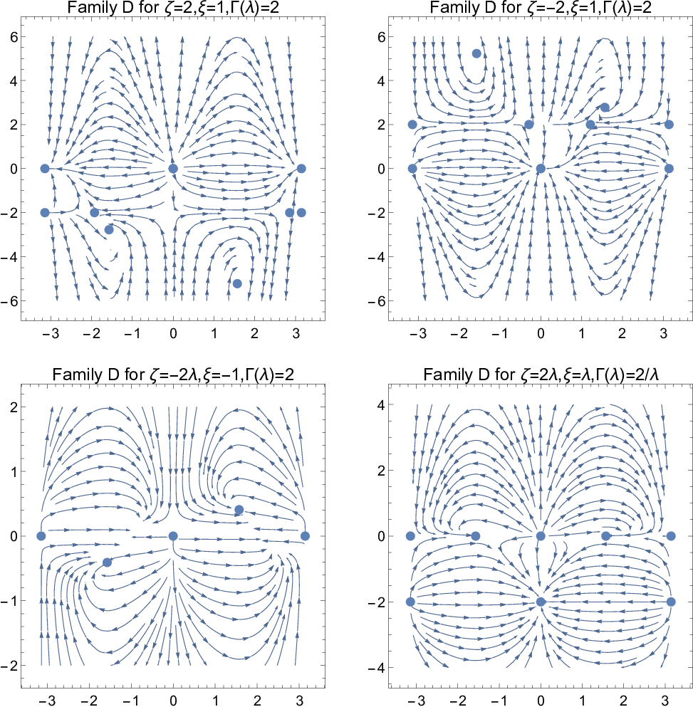
The phase-space diagram of the two-dimensional system in the variables $\left\{\omega,\lambda\right\}$ is presented in Fig. 7 for various functional forms of the free functions $\left\{\zeta\left(\lambda\right),\xi\left(\lambda\right),\Gamma^{\left(\lambda\right)}\left(\lambda\right)\right\}$ .

V Conclusions

We preformed an extended analysis on the dynamics of the Einstein-Aether cosmology with a scalar field coupled to the aether field by generalized the analysis presented in anaether. Such an analysis is important in order to understand the viability of the Einstein-æther scalar field cosmology, as also to understand the contribution of new interaction terms, between the scalar field and the aether field, in the gravitational field equations. In order to study the dynamics the cosmological evolution we studied the field equations in dimensionless form by using the $\theta-$ normalization, and we determined the stationary points. Each stationary point describe a specific phase in the cosmological history of the model.

We assumed that the scalar field and the aether field contribute in the gravitational integral a potential term of the form $V\left(\theta,\phi\right)=U\left(\phi\right)+Y\left(\phi\right)\theta+\frac{1}{3}\left(W^{2}\left(\phi\right)-1\right)\theta^{2},~$ were $U\left(\phi\right),~Y\left(\phi\right)$ and $W\left(\phi\right)$ are arbitrary function. When $W^{2}\left(\phi\right)=1,$ or in general when $W\left(\phi\right)=const$ , the analysis of anaether are recovered. In addition when $W\left(\phi\right)=const$ , $U\left(\phi\right)=V_{0}e^{-\lambda\phi}$ and $Y\left(\phi\right)=Y_{0}e^{-\frac{1}{2}\lambda\phi}$ the results of ra1 are recovered. Indeed when the function $W\left(\phi\right)=const$ , then in anaether it was found that that there are three families of stationary points, while in our consideration for the arbitrary function $W\left(\phi\right)$ there are four families of stationary points.

By writing the field equations with the use of the Einstein tensor, we observe that the contribution of $W\left(\phi\right)$ is similar with the coupling function of the scalar field with gravity in Scalar-tensor theories. While in our model the scalar field is only coupled with the aether field, however there is an undirected coupling with the gravity. In particular $W\left(\phi\right)$ can be used to define an effective varying gravitational “constant” $k_{eff}=W^{-2}\left(\phi\right)$ .

The first family of stationary points in anaether, namely Family Ā, it is consisted by two sets of stationary points which describe scaling solutions. The stationary points of Family B̄ are four pairs of stationary points, while the third family of stationary points, namely Family C̄, are again four pairs of stationary points. It is important to mention that in anaether it was assumed that parameter $y$ is always positive.

In the model of this work, the models of Families A, B and D can be seen as the generalized Families of Ā, B̄ and D̄ respectively. On the other hand, Family C describes new stationary points provided by our model and specifically by the nonconstant function $W\left(\phi\right)$ .

Family A consists two pair of stationary points which describe scaling solutions as the points of Family Ā. The stationary points of Families B and C consist five pairs of points, where the four pairs describe scaling solutions and only one pair describes de Sitter universe. However all the points have their equivalent in Families B̄ and D̄ by using the presentation of anaether. Because the dimension of the system is different from the case where $W\left(\phi\right)=const.$ the stability conditions are modified as also the physical variables, however when $W\left(\phi\right)=const,~$ we end up with the same results of anaether. Family C for the model of our consideration admits six stationary points in three pairs. The two pairs describe scaling universes while the third pair of points describe de Sitter universes. Recall that the de Sitter solution it is supported by the cosmological observations to be the attractor of the late time cosmic acceleration phase of the universe.

From our analysis we found that the introduction of the new potential term in the field equations modifies the dynamics. However, while someone will expect the stationary points to be different we found that there is an one to one correspondence between all the stationary points for the $W\left(\phi\right)=const$ and the case where $W\left(\phi\right)$ it is an arbitrary function. The only new stationary points are those of Family C.

Consequently, when $V\left(\theta,\phi\right)=U\left(\phi\right)+Y\left(\phi\right)\theta$ or $V\left(\theta,\phi\right)=U\left(\phi\right)+Y\left(\phi\right)\theta+\bar{W}^{2}\left(\phi\right)\theta^{2}$ , the cosmological history has a similar evolution. By the results of this work we can conclude that the model $V\left(\theta,\phi\right)=U\left(\phi\right)+Y\left(\phi\right)\theta+\bar{W}^{2}\left(\phi\right)\theta^{2}$ it can describe the basic cosmological history, a similar result which is expected and for the general model $V\left(\theta,\phi\right)$ , since more degrees of freedom are introduced. Of course the latter conclusion it follows from the evolution of the solution trajectories of the field equations. Recall that when $Y\left(\phi\right)=0$ , that is, $V\left(\theta,\phi\right)=U\left(\phi\right)+\bar{W}^{2}\left(\phi\right)\theta^{2}$ our model describes also the one considered by Kanno et al soda1.

The field equations of the model with $Y\left(\phi\right)=0$ in the dimensionless variables are these with $\xi=0$ . Therefore, only the stationary points of families $A,$ $C$ and $D$ exist with the additional constraint $\xi=0$ . Consequently, we can conclude that the introduction of the function $Y\left(\phi\right)$ enriches the evolution of the cosmological history.

Let us now discuss the physical interpretation of the critical points. Points $A_{1}^{\pm},~A_{2}^{\pm}$ describe scaling solutions in general, however for specific values of the free parameters these solutions can describe also de Sitter spacetimes. Consequently, for specific ranges of the free parameters the points of family $A$ can describe an unstable scaling solution which describes the inflationary era, as also a future de Sitter attractor. The situation is similar and for the rest families of critical points. Families B, C and D can admit more than two sets of critical points, but that does not mean that all those solutions can play role in the cosmological evolution, since the cosmological evolution described by the field equations it depends on the initial conditions, as it is demonstrated by the phase space diagrams presented in Figs. 3, 4 and 7. Recall that Einstein-aether have been tested as a dark energy alternative in in2.

Nevertheless, if someone would like to describe the complete cosmological history then radiation and dust fluids should be introduced in the field equations such that to describe the radiation and the matter dominated epochs. By performing a similar analysis in a scenario with more matter sources in the cosmological model, we except to find critical points where the radiation fluid or the dust fluid contribute or dominate in the cosmological evolution, such that to describe the radiation and matter eras. Further, the existence of new critical points where all the fluid sources contribute are expected to exist, similarly with the quintessence and the scalar tensor theories, for more details we refer the reader in Appendix A. On the other hand, we can require the scaling solutions that we found before to describe the additional eras of the cosmological evolution, as for example the Brans-Dicke provides an ideal gas solution or the $f\left(R\right)$ -theory which provides a radiation epoch cop2; ffr; ffr2.

Supplementary, we remark that there exist and other exact solutions for the field equations (12), (13) and (14) except from the scaling and de Sitter solutions. As it was discussed in anaether because the unknown functions are more than the equation of motions someone can construct various analytical solutions which can describe well studied cosmological solutions. For instance, if we assume $W\left(\phi\right)=W_{0}\phi\left(t\right),~\phi\left(t\right)=\phi_{0}t$ and $\theta\left(t\right)=\theta_{1}\coth\left(\theta_{0}t\right)$ such that to describe the $\Lambda$ -cosmology, it follows necessarily $U\left(\phi\right)=$ $\frac{1}{6}\left(2W_{0}^{2}\phi^{2}\left(\theta_{1}\right)^{2}\coth^{2}\left(\theta_{0}\phi\right)-3\right)$ and $Y\left(\phi\right)=-\frac{2}{3}W_{0}^{2}\phi\theta_{1}\coth\left(\theta_{0}\phi\right)\,$ , however for different functional forms of $\phi\left(t\right)$ , the $\Lambda$ -cosmology can be recovered but for different functions $U\left(\phi\right),~Y\left(\phi\right)$ . The main difference between the various classical solutions which can be found is, which is the attractor of the solution, the scaling solution $\theta\left(t\right)\simeq t^{-1}$ or the de Sitter solution $\theta\left(t\right)\simeq\theta_{1}$ .

Additional analysis which should include cosmological observations as also to study the effects of the interaction term in the perturbation level should be performed. However, such analysis is beyond the purpose of this work.

From the above results we see that maybe it is not necessary to introduce more nonlinear interactions between the scalar field and the aether field, at least in the context of the cosmological solutions.

Acknowledgements.

A.P. thanks Dr. Alex Giacomini and the Universidad Austral de Chile for the hospitality provided while this work was performed.

Appendix A Stationary points in the presence of matter

In this Appendix, we consider the existence of a dust fluid in the cosmological model, which is not interacting with the aether or the scalar fields. The only field equation which is modified it is equation (12) and becomes

\frac{1}{3}W^{2}\left(\phi\right)\theta^{2}=\frac{1}{2}\dot{\phi}^{2}+U\left(\phi\right)+\rho_{m}

(67)

where $\rho_{m}$ is the energy density of the fluid.

Because the second-order differential equations (13), (14) remain the same, when we introduce the pressureless fluid, we infer that the field equations in the dimensionless variables (19)-(23) are the same. However, the constraint equation (24) reads

\Omega_{m}=1-x^{2}-y^{2}

(68)

where now the new variable $\Omega_{m}=\frac{3\rho_{m}}{W^{2}\left(\phi\right)\theta^{2}}$ , describes the energy density of the dust fluid source constrained in the range $0\leq\Omega_{m}\leq 1.$

There are two main differences with the results presented in Section IV. Firstly, the critical points are not necessary points on the unitary circle in the two dimensional space $\left\{x,y\right\}$ , but they are located in the unitary disk with center the point $\left(0,0\right)$ . Moreover, because of the introduction of the extra variable $\Omega_{m},$ the dimension of the dynamical system has been increased by one. We present the additional points for the field equations where $\Omega_{m}$ is different from zero. However, we do not perform a complete analysis, by mean, we are not calculate the new stability conditions.

In Family A, the additional critical points are4

A_{1}^{m}=\left(-2\sqrt{\frac{2}{3}}\zeta,0\right)~,~A_{2\left(\pm\right)}^{m}=\left(-\frac{1}{\lambda}\sqrt{\frac{3}{2}},\frac{-\sqrt{3}\xi\pm\sqrt{3\left(4+\xi^{2}\right)-16\zeta\lambda}}{2\sqrt{2}\lambda}\right)

from where the energy density of the dust fluid is calculated

\Omega_{m}\left(A_{1}^{m}\right)=1-\frac{8}{3}\zeta^{2},

(69)

and

\Omega_{m}\left(A_{2\left(\pm\right)}^{m}\right)=1-\frac{3}{\lambda^{2}}+\frac{2\zeta}{\lambda}-\frac{3\xi^{2}}{4\lambda^{2}}\pm\frac{\sqrt{3}\xi}{4\lambda^{2}}\sqrt{3\left(4+\xi^{2}\right)-16\zeta\lambda}.

(70)

Point $A_{1}^{m}~$ is physical accepted when $\left|\zeta\right|\leq\frac{1}{2}\sqrt{\frac{3}{2}}$ , while for points $~A_{2\left(\pm\right)}^{m}$ when $3\left(4+\xi^{2}\right)-16\zeta\lambda\geq 0$ and $0\leq\Omega_{m}\left(A_{2\left(\pm\right)}^{m}\right)\leq 1$ . Hence, for point $A_{2\left(+\right)}^{m}$ we find the constraints $\xi\leq 0~$ : $\left\{\xi=\frac{3\left(4+\xi^{2}\right)}{16\lambda},\pm 4\lambda+\sqrt{6\left(4+\xi^{2}\right)}=0\right\}$ or $\left\{\frac{3\left(4+\xi^{2}\right)}{16\lambda}\leq\zeta\leq\frac{6-2\lambda^{2}-\left|\xi\right|\sqrt{6-\frac{9}{\lambda^{2}}}\lambda}{4\lambda},4\lambda+\sqrt{6\left(4+\xi^{2}\right)}<0\right\}$ or $\left\{\frac{6-2\lambda^{2}+\left|\xi\right|\sqrt{6-\frac{9}{\lambda^{2}}}\lambda}{4\lambda}\leq\zeta\leq\frac{3\left(4+\xi^{2}\right)}{16\lambda},-4\lambda+\sqrt{6\left(4+\xi^{2}\right)}<0\right\}$ , while when $\xi>0$ : $\left\{4\zeta\pm\sqrt{6}=0,\sqrt{6}+2\lambda=0\right\}$ or $\left\{\zeta>\frac{3\left(4+\xi^{2}\right)}{16\lambda},2\left(2\zeta+\lambda\right)\leq\frac{6+\sqrt{6-\frac{9}{\lambda^{2}}}\lambda\xi}{\lambda},4\lambda+\sqrt{6\left(4+\xi^{2}\right)}\leq 0\right\}$ or $\left\{\zeta\leq\frac{3\left(4+\xi^{2}\right)}{16\lambda},-4\lambda+\sqrt{6\left(4+\xi^{2}\right)}\leq 0,4\zeta+2\lambda+\sqrt{6-\frac{9}{\lambda^{2}}}\geq\frac{6}{\lambda^{2}}\right\}$ or $\left\{2\left(2\zeta+\lambda\right)\leq\frac{6+\sqrt{6-\frac{9}{\lambda^{2}}}\lambda\xi}{\lambda},4\zeta+2\lambda+\sqrt{6-\frac{9}{\lambda^{2}}}\geq\frac{6}{\lambda^{2}}\right\}$ with $\left\{\lambda<\pm\frac{\sqrt{6}}{2},\mp 4\lambda+\sqrt{6\left(4+\xi^{2}\right)}>0\right\}$ .

As far as concerns the physical properties of the exact solutions at those new critical points, we observe that the dust fluid as also the effective fluid of the scalar field with the aether field contribute in the cosmological solution. However, in general for this points we find that the parameter for the equation of state for the effective fluid of the scalar and the aether fields is different from zero at these points, which indicates that they are not tracking solutions, but the exact solution has a two ideal gas contribution.

In Family B we find the critical points

	$\displaystyle B_{1}^{m}$	$\displaystyle=\left(A_{1}^{m},0\right)~,~B_{2\left(\pm\right)}^{m}=\left(A_{2\left(\pm\right)}^{m},\xi_{0}\right)~,~$
	$\displaystyle B_{3}^{m}$	$\displaystyle=\left(A_{1}^{m},\xi_{0}\right)~,~B_{4\left(\pm\right)}^{m}=\left(A_{2\left(\pm\right)}^{m},0\right)~,$

where $\sqrt{2}\Gamma_{2}\left(\xi_{0}\right)\xi_{0}=\lambda$ . Easily we observe that sets of points $\left\{B_{1}^{m},B_{3}^{m}\right\}$ and $\left\{B_{2\left(\pm\right)}^{m},B_{4\left(\pm\right)}^{m}\right\}~$ has similar physical properties with points $A_{1}^{m}$ and $A_{2\left(\pm\right)}^{m}$ respectively.

For Family C the additional stationary points are

C_{1}^{m}=\left(1,0,0\right)\text{ and }C_{2\left(\pm\right)}^{m}=\left(A_{2\left(\pm\right)}^{m},0\right),

where $C_{1}^{m}$ describes a universe dominated by the pressureless fluid, while $C_{2\left(\pm\right)}^{m}$ have the same physical properties with points $A_{2\left(\pm\right)}^{m}$ . However, for points $C_{2\left(\pm\right)}^{m}~$ because $\zeta=0$ we find that the exact solutions at $C_{2\left(\pm\right)}^{m}\,\$ describe tracking solutions, that is, the effective fluid of the scalar and the aether field behaves like the dust fluid.

Finally for Family D the new critical points are found to be

	$\displaystyle D_{1}^{m}$	$\displaystyle=\left(A_{1}^{m},0\right)~,~D_{2\left(\pm\right)}^{m}=\left(A_{2\left(\pm\right)}^{m},\xi_{0}\right)~,~$
	$\displaystyle D_{3}^{m}$	$\displaystyle=\left(A_{1}^{m},\xi_{0}\right)~,~D_{4\left(\pm\right)}^{m}=\left(A_{2\left(\pm\right)}^{m},0\right)~,$

with one to one physical correspondence with points $B_{1}^{m}-B_{4\left(\pm\right)}^{m}$ .

In the generic scenario that the additinal matter source has a pressure term of the form $p_{m}=\left(\gamma-1\right)\rho_{m}$ where the limit $\gamma=1$ correspond to the dust fluid source, the field equations (19)-(23) in the dimensionless variables are modified as follows

$\displaystyle\frac{dx}{d\tau}$	$\displaystyle=\frac{1}{6}\left(x^{2}-1\right)\left(3x+2\sqrt{6}\zeta\right)-\frac{1}{6}y^{2}\left(3x+\sqrt{6}\lambda\right)+\frac{1}{2}\left(x^{2}-1\right)y\xi+\frac{\left(\gamma-1\right)}{2}x\Omega_{m},$	(71)
$\displaystyle\frac{dy}{d\tau}$	$\displaystyle=y^{2}\left(\left(1-y^{2}\right)+\frac{1}{3}x\left(3\left(x+y\xi\right)+\sqrt{6}\right)\left(\lambda+\sqrt{6}\zeta\right)\right)+y^{2}\left(\gamma-1\right)\Omega_{m}$	(72)
$\displaystyle\frac{d\lambda}{d\tau}$	$\displaystyle=\sqrt{\frac{2}{3}}x\lambda\left(\zeta+\lambda\left(\Gamma^{\left(\lambda\right)}\left(\lambda\right)-1\right)\right),$	(73)
$\displaystyle\frac{d\xi}{d\tau}$	$\displaystyle=\frac{\sqrt{3}}{6}x\xi\left(2\xi\Gamma^{\left(\xi\right)}\left(\xi\right)-\sqrt{2}\lambda\right),$	(74)
$\displaystyle\frac{d\zeta}{d\tau}$	$\displaystyle=\frac{\sqrt{6}}{3}x\Gamma^{\left(\zeta\right)}\left(\zeta\right),$	(75)

from where we find the same families of stationary points which now depend on the equation of state parameter for the ideal gas $\gamma$ .

References

(1) A. Kostelecky, Phys. Rev. D 69, 105009 (2004)
(2) S.M. Carroll, H. Tam and I.K. Wehus, Phys. Rev. D 80, 025020 (2009)
(3) D. Blas, C. Deffayet and J. Garriga, Phys. Rev. D 76, 104036 (2007)
(4) M. Mewes, Phys. Rev. D 99, 104062 (2019)
(5) S. M. Carroll and E. A. Lim, Phys. Rev. D 70, 123525 (2004)
(6) C. Heinicke, P. Baekler and F.W. Hehl, Phys. Rev. D 72, 025012 (2005)
(7) P. Horava, Phys. Rev. D 79, 084008 (2009)
(8) Luongo, M. Muccino and H. Quevedo, Phys. Dark Univ. 25, 100313 (2019)
(9) O. Luongo, G. Battista Pisani and H. Quevedo, Phys. Rev. D 93, 064057 (2016)
(10) G. Calgani, JHEP 09, 112 (2009)
(11) E. Kiritsis and G. Kofinas, Nucl. Phys. B 821, 467 (2009)
(12) E.N. Saridakis, IJMPD 20, 1485 (2011)
(13) A. Hakimov, A. Abdujabbarov and B. Ahmedov, Phys. Rev. D 88, 024008 (2013)
(14) T. Harko, Z. Kovacs and F.S.N. Lobo, Proc. Royal Soc. A: Math. Phys. Eng. Sci. 467, 0477 (2010)
(15) C. Eling and Y. Oz, JHEP 11, 067 (2014)
(16) M. M. Anber and J. F. Donoghue, Phys. Rev. D 83, 105027 (2011).
(17) M. Pospelov and Y. Shang, Phys. Rev. D 85, 105001 (2012).
(18) G. D’Odorico, F. Saueressig and M. Schutten, Phys. Rev. Lett. 113, 17, 171101 (2014).
(19) T. Griffin, P. Horava, C.M. Merby-Thompson, Phys. Rev. Lett. 110, 081602 (2013).
(20) A. O. Barvinsky, D. Blas, M. Herrero-Valea, S. M. Sibiryakov and C. F. Steinwachs, Phys. Rev. D 93, 064022 (2016).
(21) S. Mukohyama, Phys. Rev. D 80, 064005 (2009).
(22) T.P. Sotiriou, M. Visser and S. Weinfurtner, Phys. Rev. Lett. 102, 251601 (2009).
(23) T.P. Sotiriou, M. Visser and S. Weinfurtner, JHEP 0910, 033 (2009).
(24) T.P. Sotiriou, J. Phys. Conf. Ser. 283, 012034 (2011)
(25) A. Wang, Int. J. Mod. Phys. D 26, 1730014 (2014)
(26) T. Jacobson, Phys. Rev. D 81, 10502 (2010)
(27) D. Garfinkle and T. Jacobson, Phys. Rev. Lett. 107, 191102 (2011)
(28) J. Bhattacharyya, A. Coates, M. Colombo and T.P. Sotiriou, Phys. Rev. D 93, 064056 (2016)
(29) W. Donnelly and T. Jacobson, Phys. Rev. D 82, 064032 (2010)
(30) W. Donnelly and T. Jacobson, Phys. Rev. D 82, 081501 (2010)
(31) I. Carruthers and T. Jacobson, Phys. Rev. D 83, 024034 (2011)
(32) J.D. Barrow, Phys. Rev. D 85, 047503 (2012)
(33) A.R. Solomon and J.D. Barrow, Phys. Rev. D 89, 024001 (2014)
(34) X. Meng and X. Du, Phys. Lett. B 710, 493 (2012)
(35) S. Rani, A. Jawad, K. Bamba and I.U. Malik, Symmetry 11, 509 (2019)
(36) R.A. Battye, F. Pace and D, Trinh, Phys. Rev. D 96, 064041 (2017)
(37) T.G Zlosnik, P.G. Ferreira and G.K. Starkman, Phys. Rev. D 75, 044017 (2007)
(38) A. Pasqua, S. Chattopadhyay, D. Momeni, M. Raza, R. Myrzakulov and M. Faisal, JCAP 1704, 015 (2017)
(39) C. Ding, A. Wang and X. Wang, Phys. Rev. D 92, 084055 (2015)
(40) C. Eling and T. Jacobson, Class. Quantum Grav. 23, 5643 (2006); Erratum: Class. Quantum Grav. 27, 049802 (2010)
(41) A.A. Coley, G. Leon, P. Sandin and J. Latta, JCAP 1512, 010 (2015)
(42) J. Latta, G. Leon and A. Paliathanasis, JCAP 1611, 051 (2016)
(43) A. Coley and G. Leon, Gen. Rel. Grav. 51, 115 (2019)
(44) G. Leon, A. Coley and A. Paliathanasis, Annals Phys. 412, 168002 (2020)
(45) A. Coley, G. Leon, P. Sandin and J. Latta, JCAP 12, 010 (2015)
(46) T. Tamaki and U. Miyamoto, Phys. Rev. D 77, 024026 (2008)
(47) C. Ding, A. Wang, X. Wang and T. Zhu, Nucl. Phys. B 913, 694 (2016)
(48) C. Ding, Phys. Rev. D 96, 104021 (2017)
(49) M. Roumeliotis, A. Paliathanasis, P.A. Terzis and T. Christodoulakis, EPJC 79, 349 (2019)
(50) S. Kanno and J. Soda, Phys. Rev. D 94, 063505 (2006)
(51) R.J. Van Den Hoogen, A.A. Coley, B. Alhulaimi, S. Mohandas, E. Knighton and S.O. Neil, JCAO 1811, 017 (2018)
(52) B. Alhulaimi, A. Coley and P. Sandin, J. Math. Phys. 54, 042503 (2013)
(53) B. Alhulaimi, R.J. Van Den Hoogen and A.A. Coley, JCAP 1712, 045 (2017)
(54) P. Sandin, B. Alhulaimi and A.A. Coley, Phys. Rev. D 87, 044031 (2013)
(55) A. Paliathanasis, G. Papagiannopoulos, S. Basilakos and J.D. Barrow, EPJC 79, 723 (2019)
(56) E.J. Copeland, A.R. Liddle and D. Wands, Phys. Rev. D 57, 4686 (1998)
(57) O. Hrycyna and M. Szydlowski, JCAP 1312, 016 (2013)
(58) J. Wainwright and G.F.R Ellis, Cambridge University Press, Cambridge (1997)
(59) A.A. Coley, Dynamical Systems and Cosmology, Springer, Dordrecht (2003)
(60) L. Amendola and S. Tsujikawa, Dark Energy, Cambridge University Press, Cambridge (2010)
(61) G. Leon and F.O. Franz Silva, Generalized scalar field cosmologies, arXiv:1912.09856
(62) G. Leon and A. Paliathanasis, EPJC 78, 753 (2018)
(63) A. Cid, F. Izaurieta, G. Leon, P. Medina and D. Narbona, JCAP 1804, 041 (2018)
(64) A. Giacomini, S. Jamal, G. Leon, A. Paliathanasis and J. Saveedra, Phys. Rev. D 95, 124060 (2017)
(65) C.R. Fadragas and G. Leon, Class. Quantum Grav. 31, 195011 (2014)
(66) M. Abdelwahab, R. Goswani and P.K.S. Dunsby, Phys. Rev. D 85, 083511 (2012)
(67) Y.-F. Cai, E.N. Saridakis, M.R. Setare and J.-Q. Xia, Phys. Rept. 493, 1 (2010)
(68) K. Yagi, D. Blas, E. Barausse and N. Yunes, Phys. Rev. D 89, 084067 (2014)
(69) J. Oost, S. Mukohyama and A. Wang, Phys. Rev. D 97, 124023 (2018)
(70) A. Pasqua, S. Chattopadhyay, D. Momeni, M. Raza, R. Myrzakulov and M. Faizal, JCAP 1704, 015 (2017)
(71) L. Amendola, D. Polarski, S. Tsujikawa, Phys. Rev. Lett. 98, 131302 (2007)
(72) G. Papagiannopoulos, J.D. Barrow, S. Basilakos and A. Paliathanasis, Phys. Rev. D 95, 024021 (2017)