Current fluctuations in non-interacting run-and-tumble particles in one-dimension
Abstract
We present a general framework to study the distribution of the flux through the origin up to time , in a non-interacting one-dimensional system of particles with a step initial condition with a fixed density of particles to the left of the origin. We focus principally on two cases: (i) when the particles undergo diffusive dynamics (passive case) and (ii) run-and-tumble dynamics for each particle (active case). In analogy with disordered systems, we consider the flux distribution both for the annealed and the quenched initial conditions, for the passive and active particles. In the annealed case, we show that, for arbitrary particle dynamics, the flux distribution is a Poissonian with a mean that we compute exactly in terms of the Green’s function of the single particle dynamics. For the quenched case, we show that, for the run-and-tumble dynamics, the quenched flux distribution takes an anomalous large deviation form at large times , where is the rate of tumbling and is the ballistic speed between two successive tumblings. In this paper, we compute the rate function and show that it is nontrivial. Our method also gives access to the probability of the rare event that, at time , there is no particle to the right of the origin. For diffusive and run-and-tumble dynamics, we find that this probability decays with time as a stretched exponential, where the constant can be computed exactly. We verify our results for these large deviations by using an importance sampling Monte-Carlo method.
I Introduction
Current fluctuations in non-equilibrium open systems has been a major area of research in statistical physics over the last few years bodineau-derrida-prl2004; derrida-gers; derrida-gers-sep; bertini-jstatphys2006; bertini-landim-prl2005; prahofer-spohn-2002; prolhac-mallick-08; derrida-lecomte-wijland-pre2008; KM12. The probability distribution of the current of particles across a given point in space typically admits a large deviation form and the corresponding large deviation function (rate function) is often interpreted as an analogue of a free energy in non-equilibrium systems. For example, it was shown in bodineau-derrida-prl2004 that for a large one dimensional system in contact with reservoirs at unequal densities at the two ends, there exists an additivity principle obeyed by the large deviation function, much like the free energy in equilibrium systems. This additivity principle has been exploited further to compute cumulants of the current distribution prahofer-spohn-2002; prolhac-mallick-08; derrida-gers; derrida-gers-sep; bodineau-derrida-prl2004; bertini-jstatphys2006; bertini-landim-prl2005; derrida-lecomte-wijland-pre2008. Several theoretical tools have been developed to study current fluctuations, notable among them is the Macroscopic Fluctuation Theory bertini-jstatphys2006; derrida-gers; bodineau-derrida-prl2004; KM12 and the Bethe Ansatz derrida-gers-sep. Most of these studies have focused on driven diffusive systems, both interacting (as in the simple symmetric exclusion process) and non-interacting, typically in a one-dimensional setting.
Another inherently out-of-equilibrium system, much studied recently, is the so-called active run-and-tumble particle (RTP) Berg_book; TC_2008; Martens2012; patterson-gopinath, a new incarnation of the persistent random walk Sta87; Weiss. Such motion has been observed in certain bacteria such as E. Coli where the bacterium moves in straight runs, undergoes tumbling at the end of a run and chooses randomly a new direction for the next run Berg_book; TC_2008; Martens2012; patterson-gopinath; Sta87; Weiss. These motions are inherently out-of-equilibrium since they consume energy directly from the environment and self-propel themselves without any external force. There has been an enormous amount of work concerning the collective properties of an assembly of such RTPs Fodor17; bechinger_active_2016; cates_motility-induced_2015; Cates_Nature; SEB_16. Even at the single-particle level, RTP displays interesting behaviour and several single-particle observables have been studied recently. These include the position distribution for a free RTP Sta87; Martens2012; gradenigo, non-Boltzmann stationary states for an RTP in a confining potential Cates_Nature; ad-sm-gh; Mallmin_18; Sevilla_19; HP95, effects of disordered potentials Kardar-disorder, first-passage properties km-ad-sm; maes; pierre-satya-greg; ADP_2014; A2015; MLW_86, the distribution of the time at which an RTP reaches its maximum displacement anupam_rtp and RTP subjected to stochastic resetting me-sm-reset; review_resetting.
However, as far as we are aware, current fluctuations, even in a system of noninteracting RTPs have not been systematically studied. The purpose of this paper is to study the current fluctuations in the simplest setup where RTPs are noninteracting and initially confined on one-half of the real line (i.e. step-function initial condition). Such a setup was used before by Derrida and Gerschenfeld for noninteracting diffusive particles derrida-gers and they were able to compute the large-deviation form of the current or flux of particles through the origin up to time . In this paper, we use exactly the same setup, but for a more general class of noninteracting particles, which includes both diffusive as well as run-and-tumble particles, and compute analytically the flux distribution up to time .
Thus the main observable of our interest is the flux defined as the number of particles that crossed the origin (either from left or right) up to time , starting from the step initial condition where the particles are uniformly distributed over only the left side of the origin. Let us denote its probability distribution by . Clearly is a history dependent quantity, since it involves counting of all the crossings of the origin up to time . Our exact results rely on a simple but crucial observation, valid for this special step initial condition: each particle, starting from the left side of the origin, that crosses the origin an even number of times up to time does not contribute to the flux . But if it crosses the origin an odd number of times, it contributes unity to the flux . Hence, the flux is exactly equal to the number of particles present on the right side of the origin at time , i.e. . Thus the history dependent observable gets related, via this observation, to which is an instantaneous observable at time . As we will see later, it is much easier to compute the probability distribution , rather than the distribution of directly. Hence, knowing the distribution of , we can compute the flux distribution from . Note that this equivalence holds for arbitrary dynamics of the particles, for example it holds both for diffusive as well as RTP dynamics of the particles.
Based on this connection , we can apply our results for the flux distribution to another interesting problem. Consider for instance an ideal gas of noninteracting particles in a box. Imagine that the box is divided into two halves by a removable wall. Initially, all the particles are on the left half of the box and at we lift the wall and let the particles explore the full box freely. At time , we take a snapshot of the system and observe the locations of the particles. Of course, on an average, one expects that, at long times, the particles will be uniformly distributed throughout the box. We can ask: what is the probability that, at time , all the particles are again back to the left half of the box? Clearly this is an extremely rare event but what is the probability of this event? How does it decay with time? But note that this is exactly the probability . Hence, our computation of the flux distribution with step initial condition gives access to the probability of this rare event (corresponding to all the particles coming back to the left half of the box at time ), in a one-dimensional setting.
The rest of the paper is organised as follows. In section II we discuss the model and present a summary of our main results. Then in Sec. III we introduce the general setting and show how the single-particle Green’s function plays the central role in the analysis. Next in Secs. IV and V, we calculate the annealed and quenched averages, respectively, of the probability distribution of the flux for both diffusive and run-and-tumble particles. Then in Sec. VI we give the numerical verifications of our results and finally in Sec. VII we summarize and conclude.
II The model and the main results
We consider a set of noninteracting particles initially distributed uniformly with a density on the negative real axis, as in Fig. 1. Without loss of generality, we label the particles with denoting the position of the -th particle at time . Each evolves independently by a stochastic (or deterministic) evolution rule (the same law of evolution for each particle). For example, each particle can undergo independent Brownian motion. Alternatively, each particle can undergo independent RTP dynamics in one-dimension. This RTP dynamics for a single particle is defined as follows.

RTP dynamics. The position of a single RTP evolves via the Langevin equation
| (1) |
where is the intrinsic speed during a run and is a dichotomous telegraphic noise that flips from one state to another with a constant rate . The effective noise is coloured which is simply seen by computing its autocorrelation function
| (2) |
The time scale is the ‘persistence’ time of a run that encodes the memory of the noise. In the limit , but keeping the ratio fixed, the noise reduces to a white noise since
| (3) |
Thus in this so called ‘diffusive limit’, the persistent random walker reduces to an ordinary Brownian motion. For finite (i.e., persistence time scale of memory), the RTP will be referred to as an “active” particle. In the diffusive limit, the active particle dynamics reduces to an ordinary Brownian motion, which we refer to as a “passive” motion.
Given the stochastic dynamics of the individual particles, starting from the step initial condition, our main object of interest is the flux of particles through the origin up to time . If a trajectory crosses the origin from left to right, this will contribute a to the net current while if it crosses from right to left, its contribution is . The flux is thus the net contribution to the current up to time . Let us denote by the probability distribution for a given initial condition where ’s denote the initial positions of the particles at time . Following Derrida and Gerschenfeld, the effect of the initial condition on the distribution can be studied in two alternative ways, in analogy with the disordered systems where the realisation of a disorder plays an analogous role as the initial condition in our problem. It was indeed argued in derrida-gers that one has to distinguish between two different ways of averaging over the initial conditions: (i) the annealed average, where the probability distribution of the flux is averaged over all the realizations of the initial condition and (ii) the quenched average where the probability distribution is computed for the typical initial configurations. Instead of considering the distribution directly, it turns out to be convenient to consider its generating function , where the angular brackets denote an average over the history, but with fixed initial condition . The annealed and quenched averages are now defined as follows:
| (4) | |||
| (5) |
where denotes an average over the initial conditions. Note that in this problem is always an integer. As mentioned in the introduction, for the step initial condition, we can compute both and (see Fig. 2 for a plot of these probability distributions) for arbitrary dynamics of the particles by using the identity , where is the number of particles on the right side of the origin at time . Indeed, the only quantity that enters the computation for independent particles is the single particle Green’s function denoting the probability density of finding the particle at position at time , starting from at . Let us first define a central object, that will appear in all our formulas
| (6) |
obtained by integrating the Green’s function over the final position, with the initial position fixed at . If we can compute for a given dynamics, we can express and in terms of this central function . Our main results can now be summarised as follows.


Annealed case: In this case, we show that is always a Poisson distribution
| (7) |
where
| (8) |
The mean and the variance of are both given by , which can be explicitly evaluated for different types of particle motion. For example, for a Brownian motion with diffusion constant , using in Eq. (6) we get
| (9) |
where . Our result for for the diffusive case is consistent with the result of Derrida and Gershenfeld derrida-gers obtained by a different method.
In the case of the RTP dynamics, we find explicitly that at all ,
| (10) |
where and are modified Bessel functions of the first kind. Its asymptotic behaviours are given by
| (11) |
where . Thus at late times, the RTP behaves like a diffusive particle with an effective diffusion constant .
Note that the Poisson distribution in Eq. (7) in the limit , , keeping the ratio fixed, can be written in a large deviation form (using simply Stirling’s formula)
| (12) |
where the rate function is universal, i.e., independent of the particle dynamics, and is given by
| (13) |
It has the asymptotic behaviours
| (14) |
The quadratic behavior near the minimum at indicates typical Gaussian fluctuations for , with mean and variance both equal to . Note that the dependence on the particle dynamics in Eq. (12) enters only through the parameter but the function is universal.
We also note that, from our general result in Eq. (7), it follows that
| (15) |
This result is valid for all and gives the probability of the rare event that all the particles are back on the left side of the origin at time , as discussed in the introduction. In Fig. 3 (a) we show a plot of as a function of time, both for RTP and for diffusive particles.


Quenched case: In this case, the generating function in Eq. (5), for arbitrary single particle dynamics, can again be expressed in terms of the central function (6) as follows
| (16) |
The quenched cumulants of can then be extracted and expressed in terms of . For instance, the quenched mean and the variance of are given by
| (17) | |||
| (18) |
In addition, expanding the right hand side (rhs) in powers of and matching with the left hand side (lhs), one can in principle obtain for any integer as a functional of . For example,
| (19) |
which is valid for all times . However, the formula gets more complicated for higher values of . In Fig. 3 (b) we show a plot of as a function of time, both for RTP and for diffusive particles.
For the full quenched distribution, we first consider the diffusive motion of the particles. In this case, we obtain, in the scaling limit , keeping the ratio fixed, the same large deviation form as Derrida and Gerschenfeld derrida-gers,
| (20) |
where the rate function has the following precise asymptotics
| (21) |
with the two constants and given explicitly by
| (22) | |||
| (23) |
Note that the large behavior coincides with the result of Derrida and Gerschenfeld derrida-gers obtained by a different method. The small behavior was not investigated in Ref. derrida-gers. Taking the limit in Eq. (20) and using the small behavior in the first line of Eq. (21) implies that for large where the constant is given in Eq. (22). In fact, this result is valid not just at large time but at all times. Indeed, substituting in our general formula (19), it follows that at all times ,
| (24) |
Interestingly, exactly the same rate function also appeared in the completely different context, namely as a large deviation function characterising the distribution of the number of eigenvalues (in a disk of radius ) of a complex Ginibre ensemble of Gaussian random matrices castillo; bertrand.
We then consider the quenched flux distribution for the RTP dynamics. First, we show that, for small , the flux distribution decays as a stretched exponential at late times, e. g. is given, for large , by
| (25) |
where is the same constant as in Eq. (22) and . One of the main results of this analysis is to find a new scaling limit , , keeping the ratio fixed where the quenched distribution admits a large deviation form [quite different from the diffusive case in Eq. (20)]
| (26) |
where the rate function is given explicitly by
| (27) |
The rate function has the asymptotic behavior
| (28) |
One consequence of our result is the prediction of the probability of the rare event that the flux up to time achieves its maximum possible value, namely – this corresponds to the case where all the particles move ballistically to the right up to time . We find that the probability of this rare event is given by
| (29) |
Such a faster than exponential decay for the probability of this rare event is a nontrivial prediction of our theory.
III The general setting and the single-particle Green’s function
We start with a step initial condition where particles are initially located on the negative half line at positions where all . As stated before, for this step initial condition, the flux up to time is identical in law to the number of particles to the right of the origin at time . Let us introduce an indicator function such that if the particle is to the right of the origin at time , else . Hence we have
| (30) |
For fixed ’s the flux distribution is then given by
| (31) |
where the angular brackets denote an average over the history, but with fixed initial condition . Taking the Laplace transform on both sides of Eq. (31) gives
| (32) |
Since the can only take the values or , one has the identity . Inserting this identity in Eq. (32) and using the independence of the random variables ’s we get
| (33) |
where the right hand side (r.h.s.) implicitly depends on the ’s. The average is just the probability that the particle is to the right of the origin at time , starting initially at and hence we have
| (34) |
where is the single-particle Green’s function, i.e., the propagator for a particle to reach at time , starting initially at . Note that is defined in Eq. (6) and corresponds to the probability that a particle is on the positive side of the origin at time , starting initially at . Inserting Eq. (34) into Eq. (33), one obtains
| (35) |
This Eq. (35) is general, i.e., valid for any set of non-interacting particles undergoing a common dynamics in one-dimension. The information about the dynamics is entirely encoded in the function .
For instance, for simple diffusion, the single-particle Green’s function is given by
| (36) |
which gives . For the RTP, on the other hand, the Green’s function is known explicitly Weiss; me-sm-reset
| (37) |
where is given by
| (38) |
In Eq. (37), is the Heaviside Theta function, and and are modified Bessel functions. Computing explicitly using Eq. (37) is complicated. It is however much more useful, as we will see later, to work with the Laplace transform of with respect to , which has a much simpler expression, namely
| (39) |
The relation in Eq. (35) is the central result of this section and we will analyse the annealed and the quenched cases separately in the next two sections.
IV Flux distribution in the annealed case
The annealed distribution is defined in Eq. (4) where the denotes an average over the initial conditions. Performing this average in Eq. (35) gives
| (40) |
where is defined in Eq. (34). To perform the average over the initial conditions with a fixed uniform density , we assume that each of the particles is distributed independently and uniformly over a box and then eventually take the limit , keeping the density fixed. For this uniform measure, each is uniformly distributed in the box . Using the independence of the ’s we then get
| (41) |
where, in the last equality, we made the change of variable . Taking now the limit , keeping fixed gives
| (42) |
By expanding in powers of and comparing to the left hand side, we see that can take only integer values and the probability distribution is simply a Poisson distribution with mean as given in Eqs. (7) and (8).
This Poisson distribution, in the annealed case, is thus universal, i.e., holds for any dynamics. The details of the dynamics is encoded in the single parameter which can be computed explicitly for different types of dynamics. For example, for diffusing particles, using the explicit expression for the Brownian propagator, we get and, hence, as mentioned in Eq. (9). In contrast, for the RTP dynamics, is nontrivial. As discussed earlier, computing from the Green’s function in Eq. (37) is difficult. Consequently, calculating is also hard. However, it turns out that its Laplace transform is much easier to manipulate, due to the simple nature of the formula in Eq. (39). The Laplace transform of is given by
| (43) |
where we have used the relation . The Laplace transform of can be computed as follows
| (44) |
Exchanging the integrals over and , and using the relation in Eq. (39) and integrating over we get
| (45) |
Inserting this relation in Eq. (43) and performing the integral over , we get
| (46) |
This Laplace transform can be explicitly inverted, yielding the result in Eq. (10).
V Flux distribution in the quenched case
As stated in Section II, the quenched flux distribution is defined as
| (47) |
where once again represents an average over the initial positions . Our starting point is again Eq. (35). Taking the logarithm on both sides of (35) gives
| (48) |
We now perform the average over the initial positions, as in the annealed case, i.e., choosing each independently and uniformly from the box and finally taking the limit , keeping fixed. This gives
| (49) |
Therefore the Laplace transform of the quenched flux distribution is given by
| (50) |
where
| (51) |
Before extracting the full distribution from this Laplace transform, it is useful to study first the asymptotic behaviors of in the two limits : (i) and (ii) .
-
limit: In this case we expand in Eq. (51) in powers of . The two leading terms are given by
(53) where
(54) (55) Substituting this expansion (53) on the rhs of Eq. (50) and matching the powers of on both sides of Eq. (50) immediately gives
(56) (57) The first line yields the general result mentioned in Eq. (19).
These results so far are quite general, i.e., they hold for any dynamics – the dependence on the dynamics comes only through the function . In the following, we focus on two interesting dynamics, namely the diffusive and the RTP and extract the large time behavior of using Eqs. (50) and (51).
V.1 for simple diffusion
In this case, using the explicit expression , we get from Eq. (51)
| (58) |
where
| (59) |
Therefore Eq. (50) reads for all time
| (60) |
In the long time limit , we anticipate, and verify a posteriori, that takes a large deviation form in the limit where , but with the dimensionless ratio fixed
| (61) |
where is a rate function that we wish to compute. Substituting this large deviation form (61) on the left hand side (lhs) of Eq. (60) and replacing the discrete sum over by an integral (which is valid for large ), we get
| (62) |
For large , we can now evaluate the integral over in Eq. (62) by a saddle point method, which gives
| (63) |
Comparing this with the rhs of Eq. (60) we get
| (64) |
Inverting this Legendre transform one gets
| (65) |
where is given in Eq. (59).
Knowing explicitly, one can plot the large deviation function using Eq. (65) – see Fig. 4. Clearly, has a concave shape with a minimum at , the value of will be computed shortly. The asymptotic behaviors of the rate function can also be extracted in the limits , and by analysing respectively in the limits , and (where in Eq. (59) has to be continued analytically to negative ). The results are summarised in Eqs. (21), (22) and (23) in section II. Below we provide the derivation of these results.


V.1.1 Typical Fluctuations :
In order to derive the result for , we need to analyze for . We expand in Eq. (59) up to order and get
| (66) |
where
| (67) | |||
| (68) |
Substituting in Eq. (65) and maximising with respect to gives a quadratic form for the rate function
| (69) |
This form holds for close to and gives the result in the second line in Eq. (21). Substituting this quadratic behavior in the large deviation form in Eq. (61) predicts a Gaussian form for the quenched flux distribution for close to
| (70) |
where the mean the variance are given by
| (71) | |||||
| (72) |
Notice that these expressions for the mean and the variance, though derived here for large , actually hold for all , as one can verify directly from the formulae in Eqs. (17) and (18) with . Comparing with the annealed case, while the means in both cases are identical, both given by , their variances and higher moments differ. For example, the variance in the annealed case is which differs by a factor from the quenched case in Eq. (72). These results agree with those obtained in derrida-gers. This typical quadratic behavior is shown by the dashed-dotted green curve in Fig. 4.
V.1.2 Atypical fluctuations on the left of the mean:
In order to infer about the fluctuations of around , we need to evaluate how behaves when . This corresponds to the limit for from Eq. (65). We use the large expansion in Eq. 53, and evaluate and from Eq. (54) using . This gives
| (73) | |||||
| (74) |
From Eqs. (58) and (59) we get the two leading terms of for large
| (75) |
Plugging this result for in Eq. (65) and maximizing with respect to , we get the leading small behavior of
| (76) |
This reproduces the first line of Eq. (21). In particular, for , using in Eq. (61), we obtain as announced in Eq. (24). The small behavior of is shown by the solid yellow curve in Fig. 4(a).
V.1.3 Atypical fluctuations on the right of the mean:
In order to derive the large asymptotics of from Eq. (65), we first need to continue in Eq. (59) analytically to negative and use its asymptotics in the limit . For this, it is convenient to write first where . We write
| (77) |
To extract the large behavior of from the integral on the rhs, it is convenient to take the derivative with respect to
| (78) |
For large the dominant contribution to this integral comes from large where . Hence we see that, for the integrand is essentially as , while, for , the integrand is as . Hence, the integrand can be approximated by a Fermi function
| (79) |
Integrating it back, we get the leading order behavior for for large
| (80) |
Therefore as . Substituting this behavior in Eq. (65) and maximizing with respect to one gets as . This then gives the last line of the result in Eq. (21). As mentioned earlier, this leading large asymptotic behavior of coincides with the result of Ref. derrida-gers obtained by a different method. The large behavior of is shown solid the solid violet curve in Fig. 4(b).
V.2 for run-and-tumble particles
In this case, our starting point again are Eqs. (50) and (51), except that the function for the RTP is more complicated. Its Laplace transform is given in Eq. (45). As shown in Appendix C of pierre-satya-greg it can be formally inverted to obtain in real time
| (81) |
However, it turns out that this expression is not very useful to extract the large deviation function at late times.
Before proceeding to compute the large deviation function at late times, it is useful to discuss the large behavior of in different regimes of . In the following, we will first discuss the limit of , followed by the discussion of the typical fluctuations where . In this regime, we will recover the Gaussian fluctuations. When , we expect to recover the large deviation regime for the diffusive behaviour discussed in the previous section. This is because, as explained in the introduction, at late times, the RTP motion essentially reduces to that of a diffusive particle with an effective diffusion constant . However, there exists yet another “larger deviations regime” where where we will show that carries the signature of activity and has a novel large deviation form
| (82) |
In the following, we will indeed compute this rate function and show that it is given by Eq. (27).
V.2.1 Typical fluctuations:
In order to extract the typical fluctuations of around its mean value for the RTP case, we need to use the small expansion of in Eq. (50). Quite generally, the small expansion of is given in Eq. (52). We use this expansion on the rhs of Eq. (50) and approximate the sum on lhs by an integral. The resulting Laplace transform can be easily inverted and yields a Gaussian form
| (83) |
where and are given in Eqs. (17) and (18) respectively where is given in Eq. (81) – alternatively its Laplace transform is given by the simpler form in Eq. (45). The mean value can be computed explicitly. Indeed
| (84) |
where the last equality follows from Eq. (10). The variance is however difficult to compute explicitly using from Eq. (81). However, it can be easily evaluated numerically. At large times, and converge to the diffusive limits given in Eqs. (71) and (72) respectively.
V.2.2 Atypical fluctuations on the left of the mean:
Exactly at or , we have an exact expression at all times for in terms of , as given in Eqs. (56) and (57). The function for RTP appearing in these expressions is given in Eq. (81). Given this rather complicated expression of , it is hard to obtain explicit formulae valid at all times for even for or . However, at late times, since converges at late times to that of the diffusive limit in Eq. (9) with an effective diffusion constant , we recover the diffusive results for this extreme left tail of . For instance , which represents the probability of having no particle on the right side of the origin at time , decays at late times as in the diffusive case
| (85) |
where is given in Eq. (22).
V.2.3 Atypical fluctuations on the right of the mean:
In this section, we derive the result in Eq. (82). We recall that in the diffusive case, the atypical fluctuations of are encoded in the large deviation form in Eq. (61) with . The extreme fluctuations to the right of in this case are described by the large argument behavior of the large deviation function , i.e., when . Thus, in the diffusive case, there is a single scale for the fluctuations of at late times, namely . In contrast, for the RTP, in addition to the scale that describes the moderate large deviations around the mean, there is yet another scale where . This comes from the fact that each particle in time can move a maximum distance , where is the velocity. So for an initial density , the maximum possible flux through the origin is . Hence describes the scale of fluctuations at the very right tail of the distribution .
To extract this extreme right tail, we again start from Eqs. (50) and (51) with , for RTP, given by its Laplace transform in Eq. (45). Before extracting the large deviation form of , we first analyse in the limit . Inverting the Laplace transform of in Eq. (45) we get
| (86) |
where represents the Bromwich contour in the complex -plane. In the limit , with the ratio fixed, the integral can be evaluated by the saddle-point method, which yields (up to pre-exponential factors)
| (87) |
We have checked numerically that this approximation (87) works very well, at large times, as one would expect.
To extract the large behavior from Eq. (50) we need to analytically continue to negative and study the limit , as in the diffusive case. Setting with , and approximating the discrete sum on the lhs of Eq. (50) by an integral, we get
| (88) |
where
| (89) |
To extract the large behavior of we follow the same procedure as in the diffusive case and take a derivative with respect to . We get
| (90) |
For large , this integral is dominated by the region where where we can use the approximate form of given in Eq. (87). Substituting this form for in Eq. (90), we get
| (91) |
We now analyse this integral in two different cases, assuming :
If : in this case as it is clear that the integrand in Eq. (91) is always for any . Hence
| (92) |

If : this case is a bit more complicated to analyze. Since the argument of the exponential in Eq. (91) can be either positive or negative. Accordingly, the integrand will either or for large . The value of for which the argument of the exponential changes sign is given by
| (93) |
Thus, if the integrand is while for the integrand is . Hence this integral over in (91) gets cut-off at (note that for all ). Hence we get
| (94) |
Integrating it back with respect to we obtain
| (95) |
where
| (96) |
Performing these integrals explicitly, we get
| (97) |
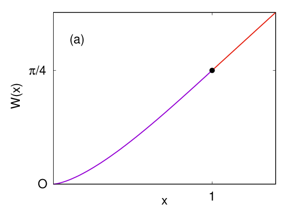
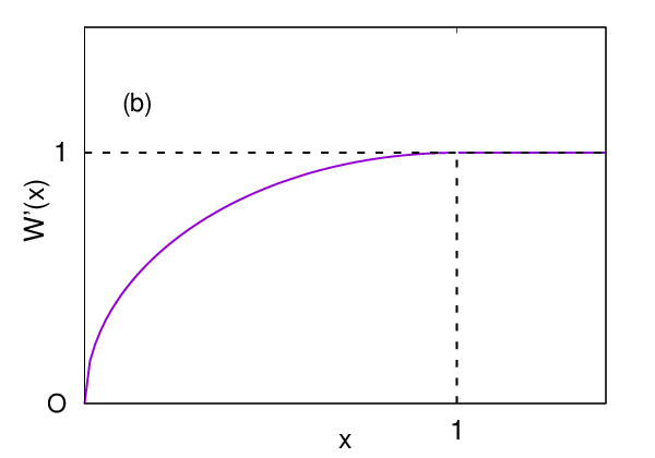
The function is plotted vs in Fig. 5 (a). Interestingly, while and its first two derivatives are continuous at , its third derivative is discontinuous. Indeed one has
| (98) |
Using this result for in Eq. (97) gives us an expression for in (95). We then substitute this expression for in Eq. (88) to get
| (99) |
Inverting formally this Laplace transform, we obtain
| (100) |
Rescaling we get, up to pre-exponential factors,
| (101) |
where is the Bromwich contour in the complex -plane. Performing this integral by using a saddle-point for large , we get
| (102) |
with the rate function given by
| (103) |
where is given explicitly in Eq. (97). It is easy to verify that the maximum of the function occurs at . Since we use the branch of in the first line of Eq. (97). Substituting this value of in Eq. (103) we get the result in Eq. (27). The asymptotic behaviours of this function are given in Eq. (28) and a plot of this function is shown in Fig. 5 (c). Note that for small , i.e. , behaves as . Substituting this behavior in Eq. (102) gives
| (104) |
On the other hand, for the diffusive case, from Eq. (20), using for large , i.e. , one gets
| (105) |
Comparing these two tails (104) and (105), one sees that for the RTP, on a scale where these two behaviors match perfectly, supporting the expectation that, at large , even for moderately large fluctuations to the right of the mean, the flux distribution for the RTP and the diffusive case coincide, once one identifies the effective diffusion constant as .
VI Numerical Results
This section is dedicated to Monte Carlo simulations. We check numerically the analytical results previously obtained and characterize the properties of the physical realizations corresponding to large values.
VI.0.1 The Importance Sampling strategy
In order to obtain the tails of and we have employed Importance Sampling, a general method used to reduce the variance of observables whose expectation value is dominated by rare realizations, in this case rare trajectories. In the context of the evaluation of large deviation functions, very popular implementations of importance sampling ideas are cloning algorithms or transition path sampling giardina2011simulating. Here we use an implementation of Importance Sampling, similar to transition path sampling, the details of the technique can be found in hartmann-epjb-2011; alberto-importance. Basically we sample realizations with an exponential bias on their flux, . The adjustable parameter allows to explore atypical realizations: a negative favours realizations with large , while a positive favours small . The sampling is done using a standard Metropolis algorithm as discussed in hartmann-epjb-2011; alberto-importance and error bars are smaller than the symbol size.
To proceed we note that the flux depends only on the particle positions at time :
| (106) |
We wrote this quantity as the sum of two contributions: (i) the initial (negative) position, and (ii) the total displacement, . The latter depends on the stochastic process we are considerning: for the diffusive particles it is a Gaussian number of zero mean and standard deviation . For active particles, it can be expressed as
| (107) |
where , is the total time spent moving in the initial particle direction, the time spent in the opposite direction. The signs or correspond to the initial direction and they are chosen with equal probability. The times and are determined as follows: the run times are drawn from an exponential distribution of rate , the last run being the first time interval for which . Then is replaced by and are computed.
The choice of the initial conditions is the delicate point that makes the annealed case different from the quenched one: in the annealed case, averages are performed over all initial conditions while in the quenched case the initial condition is fixed and typical. We first study the annealed case for active particles. At large times, their behavior is statistically equivalent to the one of diffusive particles with the effective constant . Then we discuss the quenched case and recover the exact results of previous sections. At variance with the annealed case one expects that when active particles should have a clear non-diffusive nature even at long times. Unfortunately, the biased Monte Carlo used in this paper does not allow to sample configurations with .


VI.1 Annealed case
The flux of RTPs depends on the evolution of the particles with an initial position in . But what is their number? Typically we expect , but, in the annealed case, rare realizations with large or small can occur. To capture them we consider a large interval with and draw initial positions evenly distributed in the interval. Then only the partciles with are evolved.
Here we study RTP with . At time , the average flux predicted by Eq. 10 is , very close to the one predicted in diffusive limit . Then typical realizations () are expected to be similar to the diffusive ones with . When the bias is applied () the sampled realizations have a larger flux, and it is instructive to characterize their statistical properties for RTP and diffusion.
In Fig. 6(a) we show the initial profile of particles. While for it is flat as expected, for it displays an accumulation of particles around the origin and total number of particles in the interval is much larger than . In Fig. 6(b) we show the histogram (normalized to the number of realizations) of displacement for particles with a positive final position. The peak for has the same location of the peak for . The only difference is that more particles have a positive for than for . This suggests that, in the annealed case, larger values of the flux are essentially due to rare fluctuations of the initial conditions that are completly insensitive to the nature of the particle motion.
For this reason the non-gaussian tails of the flux are Poissonian both for diffusive and active particles. In Fig. 6(c) 11 1 Note that to obtain a reliable histogram one has to re-weight the sampled values of by a factor . is a normalization constant that is determined following the method explained in hartmann-epjb-2011; alberto-importance. we observe that the agreement between simulations and Poissonian tails increases when is large, this confirms that the origin of anomalous fluctuations of the flux is in the rare realizations with large initial concentrations of particles close to the origin. This mechanism cannot work for the quenched case where the initial concentration is always flat.
VI.2 Quenched case
In the quenched case the initial condition is fixed and the number of particles with an initial position in is always . In practice, we fix the position of the first particle using a uniform random number between and and the positions of all the other particles are then slaved to according to
| (108) |
We first check the agreement between our Monte Carlo simulations and the analytical predictions. In Fig. 7 we compare the exact large deviation function and the exact probability distribution function with the ones obtained from our Monte Carlo simulations. For the quenched active case, the results are shown in Fig 8 where we also plot the large deviation function , using for the Monte Carlo data the definition with . We note that the Monte Carlo results perfectly match the predictions for both RTP and diffusion.


The difference between RTP and diffusive behaviour in the quenched case is shown is Fig. 9 (a). There we compare the exact distribution of RTP with and (red) with the diffusive one with . Both distributions deviate from the Gaussian (solid green) but they become separable from each other only at extremely small probabilities, when . The Importance Sampling strategy enables us to explore the non-Guassian tails of the distribution but not the extremely rare configurations where the finerprints of the activity are present. Indeed in Fig. 9 (b) we can hardly see a difference in histogram of the displacement of particles with positive final position between diffusion and RTP, both for and . This is because the displacements involved are still very small compare to .


VII Conclusion
In this paper, we have presented a general framework to study current fluctuations for non-interacting particles executing a common random dynamics in one dimension and starting from a step initial condition. The probability distribution depends on the initial positions of the particles . The initial positions are distributed uniformly on the negative axis with a uniform density . There are two different ways to perform the average over the initial positions, namely (i) annealed and (ii) quenched averages, in analogy with disordered systems: here the initial condition plays the role of the disorder. In the annealed case, the distribution is averaged directly over the initial positions. In contrast, in the quenched case, one considers the configurations of ’s that lead to the most likely current distribution (i.e., the typical current distribution). In both cases, we have shown that, for noninteracting particles, the distribution can be fully characterized in terms of the single particle Green’s function, which in general will depend on the dynamics of the particles. In this article, we have focused mostly on two different dynamics: a) when the single particle undergoes simple diffusion and b) when the single particle undergoes run-and-tumble dynamics (RTP).
For the annealed case, we have shown that , at all times, is given by a Poisson distribution, with parameter given by the exact formula in Eq. (8). We provide exact formula for in the RTP case (for the diffusive case this was known already from Ref. derrida-gers). For the quenched diffusive case we show that our formalism correctly recovers the large deviation result obtained in Ref. derrida-gers) using a different approach. For the RTP case, we showed that there is a new large deviation regime with , where . One of the main results of this paper is an explicit computation of the rate function given by
| (109) |
Our method gives access to another physical observable, namely the probability of an extremely rare event that there is no particle on the right side of the origin at time . We have shown that this is just the probability of having zero flux up to time , i.e. , both for the annealed and the quenched case. For the annealed case, this is just . For the quenched case, we have that, both for the diffusive and RTP cases, this probability decays at late times as a stretched exponential , where we computed the constant analytically [see Eq. (22)]. For diffusive particles, while for RTP’s, .
We have also verified our analytical predictions by numerical simulations. Computing numerically the large deviation function is far from trivial. Even for the diffusive case the large deviation function predicted for (both annealed and quenched) in Ref. derrida-gers was never verified numerically. In this paper, we used a sophisticated importance sampling method to compute numerically this large deviation function in the diffusive case up to an impressive accuracy of order . We further used the same technique to compute the large deviation function in the RTP case.
The formalism developed in this paper can be easily generalized in different directions. For instance, one can compute the flux distribution exactly for the case where there are, initially, arbitrary densities and to the left and to the right of the origin respectively, both the diffusive and for the RTP cases. One could also generalise this result in higher dimensions, with step-like initial conditions, where for instance one region of the space is initially occupied by particles with uniform density. For the diffusive case, the flux distribution in the presence of hard-core repulsions between particles was studied in Ref. derrida-gers-sep (for the simple symmetric exclusion process). It would be interesting to see whether our formalism can be generalized to study the flux distribution for RTP’s with hard core repulsions.
Acknowledgements.
We acknowledge support from the project 5604-2 of the Indo-French Centre for the Promotion of Advanced Research (IFCPAR).References
- (1) T. Bodineau and B. Derrida,Current fluctuations in non-equilibrium diffusive systems: an additivity principle, Phys. Rev. Lett. 92, 180601 (2004).
- (2) L. Bertini, A. De Sole, D. Gabrielli, G. Jona-Lasinio, and C. Landim Current fluctuations in stochastic lattice gases, Phys. Rev. Lett. 94, 030601 (2005).
- (3) L. Bertini, A. De Sole, D. Gabrielli, G. Jona-Lasinio, C. Landim, Non equilibrium current fluctuations in stochastic lattice gases, J. Stat. Phys. 123237-276 (2006).
- (4) S. Prolhac and K. Mallick, Current Fluctuations in the exclusion process and Bethe Ansatz, J. Phys. A: Math. Theor. 41 175002 (2008).
- (5) C. Appert-Rolland, B. Derrida, V. Lecomte, F. Van Wijland, Universal cumulants of the current in diffusive systems on a ring, Phys. Rev. E. 78, 021122 (2008).
- (6) B. Derrida and A. Gerschenfeld, Current Fluctuations in One Dimensional Diffusive Systems with a Step Initial Density Profile, J. Stat. Phys. 137, 978 (2009).
- (7) B. Derrida and A. Gerschenfeld, Current Fluctuations of the One Dimensional Symmetric Simple Exclusion Process with Step Initial Condition, J Stat Phys 136, 1 (2009).
- (8) M. Prähofer and H. Spohn, Current fluctuations for the totally asymmetric simple exclusion process, In and out of equilibrium, ed. V. Sidoravicius, Progress in Probability 51, 185-204, Birkhauser Boston (2002).
- (9) P. L Krapivsky, B. Meerson, Fluctuations of current in nonstationary diffusive lattice gases, Phys. Rev. E 86, 031106 (2012).
- (10) H. C. Berg, E. coli in Motion (Springer, 2014).
- (11) J. Tailleur and M. E. Cates, Statistical mechanics of interacting Run-and-Tumble bacteria, Phys. Rev. Lett. 100, 218103 (2008).
- (12) K. Martens, L. Angelani, R. Di Leonardo, and L. Bocquet, Probability distributions for the run-and-tumble bacterial dynamics: An analogy to the Lorentz model, Eur. Phys. J. E 35, 84 (2012).
- (13) A. E. Patteson, A. Gopinath, M. Goulian, P. E. Arratia, Running and tumbling with E. coli in polymeric solutions, Sci Rep. 2015 Oct 28; 5:15761. doi: 10.1038/srep15761.
- (14) W. Stadje, The exact probability distribution of a two-dimensional random walk, J. Stat. Phys. 46, 207 (1987).
- (15) G. H. Weiss, Some applications of persistent random walks and the telegrapher’s equation, Physica A: Statistical Mechanics and its Applications 311, 381 (2002).
- (16) E. Fodor, C. Marchetti, Lecture notes for the international summer school ”Fundamental Problems in Statistical Physics” held in Bruneck, Physica A 504, 106 (2018).
- (17) C. Bechinger, R. Di Leonardo, H. Löwen, C. Reichhardt, G. Volpe and G. Volpe, Active particles in complex and crowded environments, Rev. Mod. Phys. 88, 045006 (2016).
- (18) M. E. Cates, J. Tailleur, Motility-Induced Phase Separation, Annu. Rev. Conden. M. P. 6, 219 (2015).
- (19) A. P. Solon, Y. Fily, A. Baskaran, M. E. Cates, Y. Kafri, M. Kardar, J. Tailleur, Pressure is not a state function for generic active fluids Nature Phys. 11, 673 (2015).
- (20) A. B. Slowman, M. R. Evans and R. A. Blythe, Jamming and attraction of interacting run-and-tumble random walkers, Phys. Rev. Lett. 116, 218101 (2016).
- (21) G. Gradenigo, S. N. Majumdar, A first-order dynamical transition in the displacement distribution of a driven run-and-tumble particle, J. Stat. Mech.: Theor. Exp. 053206, (2019).
- (22) P. Hänggi, P. Jung, Colored noise in dynamical systems, Adv. Chem. Phys. 89, 239 (1995).
- (23) A. Dhar, A. Kundu, S. N. Majumdar, S. Sabhapandit, G. Schehr, Run-and-tumble particle in one-dimensional confining potentials: Steady-state, relaxation, and first-passage properties, Phys. Rev. E 99, 032132 (2019).
- (24) E. Mallmin, R. A. Blythe and M. R. Evans, Exact spectral solution of two interacting run-and-tumble particles on a ring, J. Stat. Mech.: Theor. Exp. 013204, (2019).
- (25) F. J. Sevilla, A. V. Arzola and E. P. Cital, Stationary superstatistics distributions of trapped run-and-tumble particles, Phys. Rev. E 99, 012145 (2019).
- (26) Y. Ben Dor, E. Woillez, Y. Kafri, M. Kardar, A. P. Solon, Ramifications of disorder on active particles in one dimension, preprint arXiv:1908.00568 (2019).
- (27) J. Masoliver, K. Lindenberg, and B. J. West, First-passage times for non-Markovian processes: Correlated impacts on a free process, Phys. Rev. A 34, 1481 (1986).
- (28) L. Angelani, R. Di Lionardo and M. Paoluzzi, First-passage time of run-and-tumble particles, Euro. J. Phys. E 37, 59 (2014).
- (29) L. Angelani, Run-and-tumble particles, telegrapher’s equation and absorption problems with partially reflecting boundaries, J. Phys. A: Math. Theor. 48, 495003 (2015).
- (30) K. Malakar et al, Steady state, relaxation and first-passage properties of a run-and-tumble particle in one-dimension J. Stat. Mech. (2018) 043215
- (31) T. Demaerel and C. Maes, Active processes in one dimension, Phys. Rev. E. 97, 032604 (2018).
- (32) P. Le Doussal, S. N. Majumdar, G. Schehr, Non-crossing run-and-tumble particles on a line, arXiv:1902.06176 (2019).
- (33) P. Singh, A. Kundu, Generalised “Arcsine” laws for run-and-tumble particle in one dimension, J. Stat. Mech., 083205 (2019).
- (34) M. R. Evans and S. N. Majumdar, Run and tumble particle under resetting: a renewal approach, J. Phys. A: Math. Theor. 51, 475003 (2018).
- (35) For a recent review on stochastic resetting, see M. R. Evans, S. N. Majumdar, G. Schehr, Stochastic resetting and applications, J. Phys. A: Math. Theor. in press https://doi.org/10.1088/1751-8121/ab7cfe (2020).
- (36) B. Lacroix-A-Chez-Toine, J. Andres Monroy Garzon, C. Sebastian Hidalgo Calva, I. Perez Castillo, A. Kundu, S. N. Majumdar, G. Schehr, Intermediate deviation regime for the full eigenvalue statistics in the complex Ginibre ensemble, Phys. Rev. E 100, 012137 (2019).
- (37) B. Lacroix-A-Chez-Toine, S. N. Majumdar, G. Schehr, Rotating trapped fermions in two dimensions and the complex Ginibre ensemble: Exact results for the entanglement entropy and number variance, Phys. Rev. A 99, 021602(R) (2019).
- (38) C. Giardinà, J. Kurchan, V. Lecomte, J. Tailleur, Simulating rare events in dynamical processes, J. Stat. Phys., 145, 787, (2011).
- (39) A. K. Hartmann et al, High-precision simulation of the height distribution for the KPZ equation, Euro. Phys. Lett. 121 (2018).
- (40) A. K. Hartmann, Large-deviation properties of largest component for random graphs, Eur. Phys. J. B 84, 627 (2011).