Discovering Nonlinear Relations with Minimum Predictive Information Regularization

We consider $N$ time series $x^{(1)},x^{(2)},...x^{(N)}$, where each time series $x^{(i)}=(x^{(i)}_{1},x^{(i)}_{2},...x^{(i)}_{t},...)$ and each $x^{(i)}_{t}\in\mathbb{R}^{M}$ is an $M$-dimensional vector. Denote $X_{t-1}^{(i)}=(x^{(i)}_{t-K},x^{(i)}_{t-K+1},...x^{(i)}_{t-1})$ with maximum time horizon of $K$, and $\mathbf{X}_{t-1}=\{X_{t-1}^{(i)}\},i=1,2,...N$. We also denote $\mathbf{X}_{t-1}^{(\hat{j})}=\mathbf{X}_{t-1}\texttt{\textbackslash}X^{(j)}_{t-1}$ ($\mathbf{X}_{t-1}$ excluding $X^{(j)}_{t-1}$). We assume that $x^{(1)},x^{(2)},...x^{(N)}$ are generated by stationary response functions $h_{i}$ that are unknown to the learner:

for $t=K+1,K+2,...$ . Here $u_{i}\in\mathbb{R}^{M},i=1,2,...N$ are noise variables that are mutually independent, are independent of any $X^{(i)}_{t-1},x^{(i)}_{t}$, $i\in\{1,2,...N\}$. For any $i,j\in\{1,2,...N\}$, we assume that the variables $(\mathbf{X}_{t-1}^{(\hat{j})},X_{t-1}^{(j)},x_{t}^{(i)})$ have probability density function $P(\mathbf{X}_{t-1}^{(\hat{j})},X_{t-1}^{(j)},x_{t}^{(i)})$.

Our method is inspired by Granger causality [11, 12], which defines causality via predictions, making it especially suitable for relational inference of observational time series. Adapting to our notation:

Granger causality [12]: Assuming causal sufficiency [35], we say $X^{(j)}_{t-1},j\neq i$ does not Granger-cause $x^{(i)}_{t}$, if $P(x^{(i)}_{t}|X^{(j)}_{t-1},\mathbf{X}_{t-1}^{(\hat{j})})=P(x^{(i)}_{t}|\mathbf{X}_{t-1}^{(\hat{j})})$. Otherwise, we say $X^{(j)}_{t-1}$ Granger-causes $x^{(i)}_{t}$.

In practice, we say that time series $j$ Granger-causes time series $i$, if it can be shown via significance tests that the null hypothesis of $P(x^{(i)}_{t}|X^{(j)}_{t-1},\mathbf{X}_{t-1}^{(\hat{j})})=P(x^{(i)}_{t}|\mathbf{X}_{t-1}^{(\hat{j})})$ is rejected, i.e. $X_{t-1}^{(j)}$ provides statistically significant information for predicting $x_{t}^{(i)}$.

In his original work, Granger [11] investigates causality with linear function predictors. Later works have extended it to kernel methods [1, 25, 26, 43], which essentially estimate linear Granger causality on the feature space of the kernel. To learn potentially highly nonlinear response functions, it may be desirable to use expressive and universal function approximators [18] such as neural nets. Neural nets are much more flexible than linear models, and do not require kernel selection as in kernel methods.

Based on the definition of Granger causality, a naïve way to combine it with neural net is: for each $j\to i$, train two neural nets, one predicting $x_{t}^{(i)}$ based on $\mathbf{X}_{t-1}^{(\hat{j})}$, another predicting $x_{t}^{(i)}$ based on the full $\mathbf{X}_{t-1}=(\mathbf{X}_{t-1}^{(\hat{j})},X_{t-1}^{(j)})$, and test whether former MSE is significantly larger than the latter. This method suffers from two major drawbacks: (1) instability: different training of the neural net may end up in different local minima, so that the two MSEs have large variance, which is observed in our initial explorations; (2) inefficiency: to discover the relations among $N$ time series, it has to train at least $N^{2}$ models (for each $x^{(i)}_{t}$, train $N-1$ models with one $X_{t-1}^{(j)}$ removed, and $Q$ models ($Q\geq 1$) with full $\mathbf{X}_{t-1}$ for accumulating statistics). On the other hand, these two drawbacks exactly inspire our method. Instead of predicting $x^{(i)}_{t}$ with one $X_{t-1}^{(j)}$ missing at a time, what if we let each $X_{t-1}^{(j)}$ have learnable corruption, and encourage each $X_{t-1}^{(j)}$ to provide as little information to $x^{(i)}_{t}$ as possible while maintaining good prediction? In this way, we have a single shared model that can span the full product space of $[\text{total corruption},\text{no corruption}]^{\bigotimes N}$ for $N$ input time series, which is more stable and efficient than the removing one $X_{t-1}^{(j)}$ at a time and training $N$ models. To achieve this, we add independent noise with learnable amplitudes to each input $X_{t-1}^{(j)}$, and measure the corruption by the mutual information between the input and the corrupted input. We then define the following risk:

where $\tilde{\mathbf{X}}^{(\bm{\eta})}_{t-1}:=\mathbf{X}_{t-1}+\bm{\eta}\odot\bm{\epsilon}$ (or element-wise, $\tilde{X}_{t-1}^{(j)(\eta_{j})}:=X_{t-1}^{(j)}+\eta_{j}\cdot\epsilon_{j}$, $j=1,2,...N$) is the noise-corrupted inputs with learnable noise amplitudes $\eta_{j}\in\mathbb{R}^{KM}$, and $\epsilon_{j}\sim N(\mathbf{0},\mathbf{I})$. $\lambda>0$ is a positive hyperparameter for the mutual information $I(\cdot,\cdot)$. Intuitively, the minimization of the second term $I(\tilde{X}^{(j)(\eta_{j})}_{t-1};X^{(j)}_{t-1})$ requires the noise amplitude $\eta_{j}$ to go up. The minimization of the first term requires the noise amplitude $\eta_{j}$ to go down, and the larger causal strength from $X_{t-1}^{(j)}$ to $x_{t}^{(i)}$, the larger this force. The minimization of the two terms strikes a balance, at which point the $I(\tilde{X}^{(j)(\eta_{j})}_{t-1};X^{(j)}_{t-1})$ measures the minimum number of bits of information the time series $j$ need to provide to the learner, without compromising the prediction.

At the minimization of $R_{\mathbf{X},x^{(i)}}[f_{\theta},\bm{\eta}]$, we define $W_{ji}=I\left(\tilde{X}^{(j)(\eta_{j}^{*})}_{t-1};X^{(j)}_{t-1}\right)$, which we term minimum predictive information, where $(f_{\theta^{*}},\bm{\eta}^{*})=\text{argmin}_{(f_{\theta},\bm{\eta})}R_{\mathbf{X},x^{(i)}}[f_{\theta},\bm{\eta}]$. Essentially, $W_{ji}$ measures the predictive strength of time series $j$ for predicting time series $i$, conditioned on all the other observed time series. We have that $W_{ji}$ satisfies the following properties:

1. (1)

   If $x^{(j)}\mathchoice{\mathrel{\hbox to0.0pt{$\displaystyle\perp$\hss}\mkern 2.0mu{\displaystyle\perp}}}{\mathrel{\hbox to0.0pt{$\textstyle\perp$\hss}\mkern 2.0mu{\textstyle\perp}}}{\mathrel{\hbox to0.0pt{$\scriptstyle\perp$\hss}\mkern 2.0mu{\scriptstyle\perp}}}{\mathrel{\hbox to0.0pt{$\scriptscriptstyle\perp$\hss}\mkern 2.0mu{\scriptscriptstyle\perp}}}x^{(i)}$, then $W_{ji}=0$.

2. (2)

   $W_{ji}$ is invariant to affine transformation of each individual $X_{t-1}^{(k)},k=1,2,...N$.

3. (3)

   $W_{ji}$ is invariant to reparameterization of $\theta$ in $f_{\theta}$ (the mapping remains the same).

The proofs are provided in Appendix B. Property 1 shows that $W_{ji}$ is able to differentiate time series that are dependent or independent with the target time series $i$. Empirically, to perform statistical tests, we can let the null hypothesis be $x^{(j)}\mathchoice{\mathrel{\hbox to0.0pt{$\displaystyle\perp$\hss}\mkern 2.0mu{\displaystyle\perp}}}{\mathrel{\hbox to0.0pt{$\textstyle\perp$\hss}\mkern 2.0mu{\textstyle\perp}}}{\mathrel{\hbox to0.0pt{$\scriptstyle\perp$\hss}\mkern 2.0mu{\scriptstyle\perp}}}{\mathrel{\hbox to0.0pt{$\scriptscriptstyle\perp$\hss}\mkern 2.0mu{\scriptscriptstyle\perp}}}x^{(i)}$. Before training, we append to $\mathbf{X}_{t-1}$ some fake time series $v^{(s)}_{t-1},s=1,2,...S$ (e.g. by randomly permuting $X_{t-1}^{(j)}$) so that $v^{(s)}_{t-1}\mathchoice{\mathrel{\hbox to0.0pt{$\displaystyle\perp$\hss}\mkern 2.0mu{\displaystyle\perp}}}{\mathrel{\hbox to0.0pt{$\textstyle\perp$\hss}\mkern 2.0mu{\textstyle\perp}}}{\mathrel{\hbox to0.0pt{$\scriptstyle\perp$\hss}\mkern 2.0mu{\scriptstyle\perp}}}{\mathrel{\hbox to0.0pt{$\scriptscriptstyle\perp$\hss}\mkern 2.0mu{\scriptscriptstyle\perp}}}x^{(i)}_{t}$. After optimizing w.r.t. to the augmented dataset, the values of $W_{si}$ between $v^{(s)}_{t-1}$ and $x_{t}^{(i)}$ form a distribution for which we know that the null hypothesis is true. Then if certain $W_{ji}$ is greater than the $1-\alpha$ quantile (e.g. $\alpha=0.05$) of the distribution, we can reject the null hypothesis of independence. Properties 2 and 3 show the benefit of our method which essentially regularizes the input information, compared with L1 and group L1 [27, 40, 46] which regularize the model and thus do not satisfy these two properties.

Moreover, in Appendix B we further provide intuition that under certain conditions, $W_{ji}$ is likely to favor the time series that directly causes time series $i$, compared with the time series that relate to $i$ via the direct causal connections. Note that our method is not guaranteed to identify direct causal relations (in Granger [12] or Pearl [32] sense), which is a very hard problem given the potential large number of time series and nonlinearity present. However, our method provides an effective data exploratory tool to identify time series that are predictive of one another, conditioned on all the other observed time series, whose identified directional relations can be investigated further by a researcher. As stated above, under certain conditions, our method does favor the direct causal relations. And in the experiment section, we will compare the estimated $W_{ji}$ with true causal relations if available.

Empirically, we minimize the following empirical risk:

In general, it may be inefficient to estimate the mutual information $I(\tilde{X}^{(j)(\eta_{j})}_{t-1};X^{(j)}_{t-1})$ with large dimension of $X^{(j)}_{t-1}$ such that the expression is also differentiable w.r.t. $\eta_{j}$. Utilizing the property of Gaussian channels, in Appendix C we prove that $I(\tilde{X}^{(j)(\eta_{j})}_{t-1};X^{(j)}_{t-1})\leq\frac{1}{2}\sum_{l=1}^{KM}\text{log}\left(1+\frac{\text{Var}(X_{t-1,l}^{(j)})}{\eta_{j,l}^{2}}\right)$, where $l$ denotes the $l^{\text{th}}$ element of a vector, and $\text{Var}(X_{t-1,l}^{(j)})$ is the variance of $X_{t-1,l}^{(j)}$ across $t$. Therefore, in practice to improve efficiency, we can optimize an upper bound of the risk:

When the dimension of $X_{t-1}^{(j)}$ is large, a differentiable estimate of the mutual information (e.g. MINE [3]) can be applied. We provide Algorithm 1 to empirically estimate $W_{ji}$, which we term relational learning with Minimum Predictive Information Regularization (MPIR). The steps 1-3 construct fake input time series $v_{t-1}^{(s)},s=1,2,...S$ (which we know the null hypothesis of $v_{t-1}^{(s)}\mathchoice{\mathrel{\hbox to0.0pt{$\displaystyle\perp$\hss}\mkern 2.0mu{\displaystyle\perp}}}{\mathrel{\hbox to0.0pt{$\textstyle\perp$\hss}\mkern 2.0mu{\textstyle\perp}}}{\mathrel{\hbox to0.0pt{$\scriptstyle\perp$\hss}\mkern 2.0mu{\scriptstyle\perp}}}{\mathrel{\hbox to0.0pt{$\scriptscriptstyle\perp$\hss}\mkern 2.0mu{\scriptscriptstyle\perp}}}{}x_{t}^{(i)}$ is true) to append to $\mathbf{X}_{t-1}$. Steps 4-9 optimize the objective w.r.t. the augmented dataset, and obtain a $(N+S)\times N$ matrix $W_{ji}$. Step 10 performs significance test and only preserve the $W_{ji}$ values in the main $N\times N$ matrix that are statistically significant. In the case where we only need to estimate the predictive strength, this step is not required. Finally the main matrix is returned.

To select an appropriate hyperparameter $\lambda$, we can additionally append to the target $x_{t}^{(i)}$ a few time series $w_{t}$ constructed from $\mathbf{X}_{t-1}$. We then select $\lambda$ such that the estimated causal strength between $\mathbf{X}_{t-1}$ and $w_{t}$ (for which we know the causal relations) is at least $4\sigma$ away from the estimated causal strength between $v_{t-1}$ and $w_{t}$ (for which we know that they are independent). See Appendix A for details.

In this experiment, we evaluate our method together with other methods using a nonlinear synthetic dataset generated to have a known causal structure (hidden to the methods being compared). We study performance with varying number $N$ of time series, with $N$ up to $30$. To generate the data, we let each $x_{t}^{(i)}$ have dimension $M=1$, and also set the maximum time horizon $K=3$, so each $X_{t-1}^{(j)}$ is a $K\times M=3\times 1$ matrix. We use the following realization of the response function $h_{i}$ in Eq. (1):

where $u_{t}\sim N(\mathbf{0},\mathbf{I})\in\mathbb{R}^{M}$, $\odot$ denotes element-wise multiplication, and $\text{H}_{1}$ and $\text{H}_{2}$ are two nonlinear functions to make the response functions nonlinear. In this experiment, we use $\text{H}_{1}(x)=\text{softplus}(x)=\text{log}(1+e^{x})$, and $\text{H}_{2}(x)=\text{tanh}(x)$. $B_{j}$ is a $K\times M$ random matrix, whose element is sampled from $U[-1,1]$. $A_{ji}$ is a $K\times M$ matrix, with 0.5 probability of being a zero matrix and 0.5 probability of being a nonzero random matrix, characterizing the underlying causal strength from $j$ to $i$. Crucially, to reflect that the causal strength may span different orders of magnitude, if $A_{ji}$ is sampled to be a nonzero matrix, then the amplitude of each of its element is sampled from a log-normal distribution with $\mu=1,\sigma=0$, their sign sampling from $U\{-1,1\}$. Denote $\mathbbm{1}(A)$ as the 0-1 indicator matrix of causality ($\mathbbm{1}(A)_{ji}=1\ \text{if}\ |A_{ji}|>0;0\ \text{otherwise}$). The goal of each algorithm being evaluated is to produce an $N\times N$ score matrix $\tilde{A}$, where each entry $\tilde{A}_{ji}$ characterizes the directional strength from $j$ to $i$. Then the flattened $\tilde{A}$ is evaluated against the flattened $\mathbbm{1}(A)$ (excluding diagonal elements of the matrices) via different metrics. Fig. S4 in Appendix E shows example snapshots of the time series.

In general, for a large $N$, the number of possible causal graphs grows double exponentially: there are $2^{N^{2}}$ possible matrix of $\mathbbm{1}(A)$. To give an estimate, for $N=3,4,5,8,10,20,30$, there are $512,6.6\times 10^{4},3.3\times 10^{7},1.8\times 10^{19},1.2\times 10^{30},2.6\times 10^{120},8.5\times 10^{270}$ number of possible graphs, respectively. Therefore, estimating the underlying causal graph is in general a non-trivial task when $N$ is large. We compare our algorithm with previous methods including transfer entropy [41], causal influence [20], linear Granger causality [11, 9], kernel Granger causality [25, 26], and three baselines: (1) mutual information $\tilde{A}_{ji}=I(X_{t-1}^{(j)};x_{t}^{(i)})$ (which gives $\tilde{A}_{ji}=\tilde{A}_{ij}$), (2) a sparse feature selection method, elastic net [53], and (3) a random matrix, each element of which is drawn from a standard Gaussian distribution. For each $N$, we sample 10 datasets with different $A_{ji}$ and $B_{j}$ matrices, and compare each method’s average performance over 10 datasets together with their standard deviation. The implementation details for each method and each experiment are provided in Appendix D and E, respectively. Since many of the methods do not provide a threshold or significance test, we use the standard metrics of area under the precision-recall curve (AUC-PR) [8] (Table 1 below) and area under the ROC curve (AUC-ROC) (Table S1 in Appendix F) to compare their performance.

We see that for smaller $N$ ($N\leq 4$), methods with smaller expressivity (linear Granger, kernel Granger) performs slightly better. However, as $N$ becomes larger, our method outperforms other methods with increasing margin, demonstrating our method’s capability to infer complex relational structures from interacting time series. Particularly, although two linear methods, linear Granger and elastic net, have relatively strong performance with $N\leq 5$, they quickly degrade with larger $N$ due to more nonlinearity present in the data. With the help of kernels, kernel Granger degrades slower, but can not compete in larger $N$ with our method which allows expressive neural nets to model complex nonlinear interactions. For the Causal Influence method, although it has very good mathematical properties, it may be impractical in practice, as is also shown in the table. This is due to that it is defined as the KL-divergence between $(\mathbf{X}_{t-1},x_{t-1}^{(i)})$ and its counterpart (whose causal arrows to and from time series $j$ are cut), each of which is an $(NK+1)M-$dimensional vector, which can quickly go to high dimensions, where density estimation required to calculate KL-divergence is in general data-hungry and difficult. In comparison, our method that estimates predictive strength via minimizing prediction errors is comparatively easier in high dimensions.

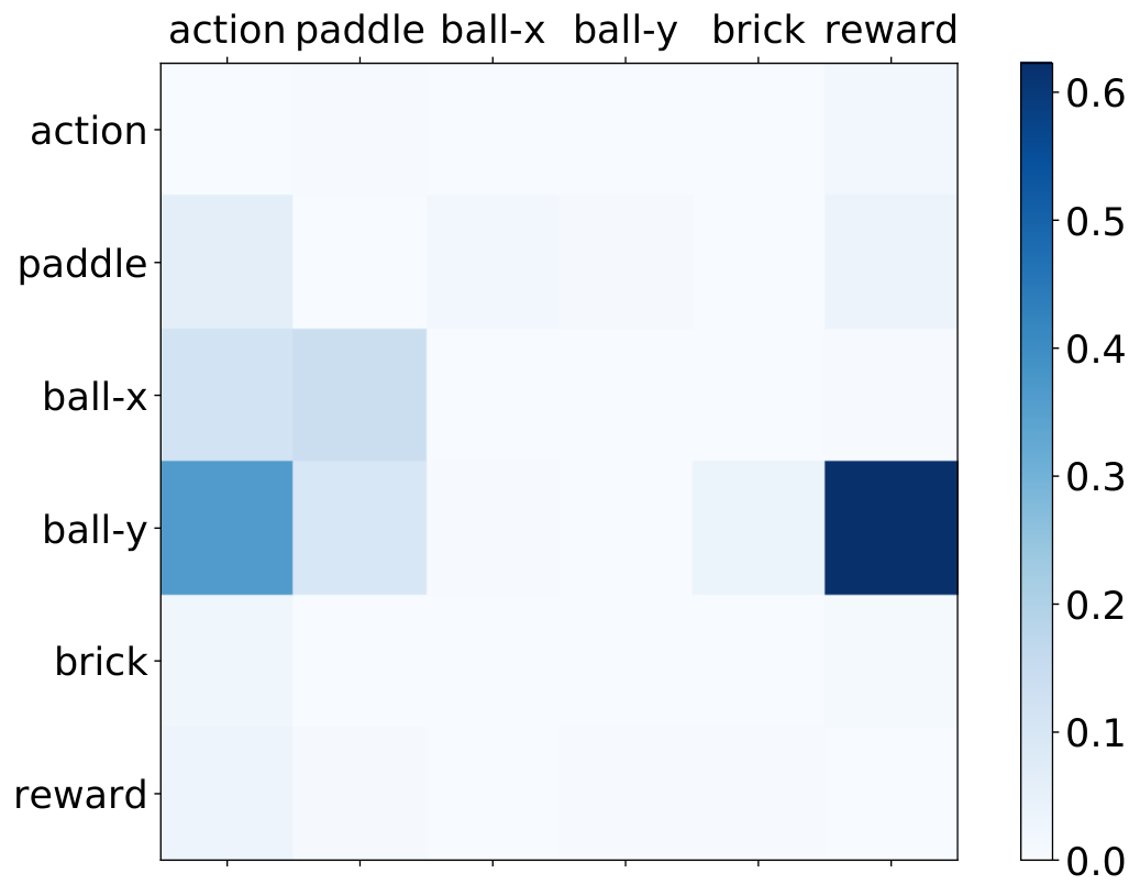
To see how our method can discover the directional (possibly causal) relations in real video games, and potentially improve reinforcement learning (RL) or imitation learning (IL), we apply our method to the relational inference between the trajectories of different objects from a trained CNN RL-agent playing Atari Breakout games ([4], implementation details see Appendix H). Fig. 1 shows the inferred $W_{ji}$ matrix for our method and compared methods, respectively. The true underlying causal chain is marked in dark color in Fig. 1e, with light color marking the competing causal relations that are indistinguishable from data (e.g. decrease of bricks and increase of reward happen at the same time step, so we cannot distinguish ball-y$\to$brick and ball-y$\to$reward). Compared with other methods, we see that our method is able to discover comparatively most of the causal relations without finding false positives. Specifically, it correctly discovers a prominent causal direction from the ball’s $y$ position to the reward, as well as brick $\to$ reward, ball-x $\to$ action, ball-y $\to$ action. The latter two show that the ball’s $x$ and $y$ positions also have influences on the trained agent’s action: in order that the ball does not fall to the bottom, the agent has to position itself at the right position depending on the $x$ and $y$ positions of the ball.

In comparison, mutual information (Fig. 1b) gives a symmetric matrix that does not differentiate the two possible directions, and also misses the arrows ball-y$\to$brick$\to$reward. For transfer entropy (Fig. 1c), although it correctly discovers a number of causal arrows, it also gives relatively high scores for some incorrect arrows: brick$\to$ action, ball-y$\to$ball-x. For kernel Granger (Fig. 1f), although it correctly discovers four causal relations, it also incorrectly finds reward$\to$ball-y and reward$\to$brick. For elastic net (Fig. 1g), it correctly discovers two prominent causal relations: ball-y$\to$action and ball-y$\to$reward, but misses a few others. Linear Granger (Fig. 1d) and causal influence (Fig. 1h) fail to discover useful causal arrows.

Now we test our algorithm with real-world datasets. As a common dataset studied in previous causal works, we use the time-series of the breath rate and instantaneous heart rate of a sleeping patient suffering from sleep apnea (samples 2350-3550 of data set B from Santa Fe Institute time series contest held in 1991, available in [36]). We apply our method to infer the directional relations between the breath rate and heart rate, with different maximum time horizon $K$. The result is shown in Fig. 2. We see that the predictive strength $W_{ji}$ from heart to breath is significantly higher than the reverse direction that is basically 0, consistent with the results from previous causal inference methods [41, 1, 25] as also shown in Fig. 2(b)(c). Notably, the $W_{ji}$ from heart to breath estimated by our method remains at roughly the same level for different $K$s, in contrast to the decaying causality index w.r.t. increasing history length in ([1], Fig. 2 (c)), showing a merit of our method in estimating directional strength across different time-horizons, aided by the flexibility of neural nets in extracting the right information to predict the future. The implementation details are provided in Appendix I. In addition, in Appendix J we test our algorithm on a rat EEG dataset, and obtain consistent result with previous works.

References

- Ancona et al. [2004] Ancona, N., Marinazzo, D., and Stramaglia, S. Radial basis function approach to nonlinear granger causality of time series. Physical Review E, 70(5):056221, 2004.
- Battaglia et al. [2016] Battaglia, P., Pascanu, R., Lai, M., Rezende, D. J., et al. Interaction networks for learning about objects, relations and physics. In Advances in neural information processing systems, pp. 4502–4510, 2016.
- Belghazi et al. [2018] Belghazi, I., Rajeswar, S., Baratin, A., Hjelm, R. D., and Courville, A. Mine: mutual information neural estimation. arXiv preprint arXiv:1801.04062, 2018.
- Bellemare et al. [2013] Bellemare, M. G., Naddaf, Y., Veness, J., and Bowling, M. The arcade learning environment: An evaluation platform for general agents. Journal of Artificial Intelligence Research, 47:253–279, 2013.
- Brockman et al. [2016] Brockman, G., Cheung, V., Pettersson, L., Schneider, J., Schulman, J., Tang, J., and Zaremba, W. Openai gym, 2016.
- Chang et al. [2016] Chang, M. B., Ullman, T., Torralba, A., and Tenenbaum, J. B. A compositional object-based approach to learning physical dynamics. arXiv preprint arXiv:1612.00341, 2016.
- Chickering [2002] Chickering, D. M. Optimal structure identification with greedy search. Journal of machine learning research, 3(Nov):507–554, 2002.
- Davis & Goadrich [2006] Davis, J. and Goadrich, M. The relationship between precision-recall and roc curves. In Proceedings of the 23rd international conference on Machine learning, pp. 233–240. ACM, 2006.
- Ding et al. [2006] Ding, M., Chen, Y., and Bressler, S. L. Granger causality: basic theory and application to neuroscience. Handbook of time series analysis: recent theoretical developments and applications, pp. 437–460, 2006.
- Diuk et al. [2008] Diuk, C., Cohen, A., and Littman, M. L. An object-oriented representation for efficient reinforcement learning. In Proceedings of the 25th international conference on Machine learning, pp. 240–247. ACM, 2008.
- Granger [1969] Granger, C. W. Investigating causal relations by econometric models and cross-spectral methods. Econometrica: Journal of the Econometric Society, pp. 424–438, 1969.
- Granger [1980] Granger, C. W. Testing for causality: a personal viewpoint. Journal of Economic Dynamics and control, 2:329–352, 1980.
- Granger et al. [2000] Granger, C. W., Huangb, B.-N., and Yang, C.-W. A bivariate causality between stock prices and exchange rates: evidence from recent asianflu. The Quarterly Review of Economics and Finance, 40(3):337–354, 2000.
- Guttenberg et al. [2016] Guttenberg, N., Virgo, N., Witkowski, O., Aoki, H., and Kanai, R. Permutation-equivariant neural networks applied to dynamics prediction. arXiv preprint arXiv:1612.04530, 2016.
- Harris & Drton [2013] Harris, N. and Drton, M. Pc algorithm for nonparanormal graphical models. The Journal of Machine Learning Research, 14(1):3365–3383, 2013.
- Hauser & Bühlmann [2012] Hauser, A. and Bühlmann, P. Characterization and greedy learning of interventional markov equivalence classes of directed acyclic graphs. Journal of Machine Learning Research, 13(Aug):2409–2464, 2012.
- Hiemstra & Jones [1994] Hiemstra, C. and Jones, J. D. Testing for linear and nonlinear granger causality in the stock price-volume relation. The Journal of Finance, 49(5):1639–1664, 1994.
- Hornik [1991] Hornik, K. Approximation capabilities of multilayer feedforward networks. Neural networks, 4(2):251–257, 1991.
- Hoshen [2017] Hoshen, Y. Vain: Attentional multi-agent predictive modeling. In Advances in Neural Information Processing Systems, pp. 2701–2711, 2017.
- Janzing et al. [2013] Janzing, D., Balduzzi, D., Grosse-Wentrup, M., Schölkopf, B., et al. Quantifying causal influences. The Annals of Statistics, 41(5):2324–2358, 2013.
- Kingma & Ba [2014] Kingma, D. P. and Ba, J. Adam: A method for stochastic optimization. arXiv preprint arXiv:1412.6980, 2014.
- Kraskov et al. [2004] Kraskov, A., Stögbauer, H., and Grassberger, P. Estimating mutual information. Physical review E, 69(6):066138, 2004.
- Lizier et al. [2008] Lizier, J. T., Prokopenko, M., and Zomaya, A. Y. Local information transfer as a spatiotemporal filter for complex systems. Physical Review E, 77(2):026110, 2008.
- Lozano et al. [2009] Lozano, A. C., Abe, N., Liu, Y., and Rosset, S. Grouped graphical granger modeling for gene expression regulatory networks discovery. Bioinformatics, 25(12):i110–i118, 2009.
- Marinazzo et al. [2008a] Marinazzo, D., Pellicoro, M., and Stramaglia, S. Kernel method for nonlinear granger causality. Physical review letters, 100(14):144103, 2008a.
- Marinazzo et al. [2008b] Marinazzo, D., Pellicoro, M., and Stramaglia, S. Kernel-granger causality and the analysis of dynamical networks. Physical review E, 77(5):056215, 2008b.
- Meier et al. [2008] Meier, L., Van De Geer, S., and Bühlmann, P. The group lasso for logistic regression. Journal of the Royal Statistical Society: Series B (Statistical Methodology), 70(1):53–71, 2008.
- Mnih et al. [2015] Mnih, V., Kavukcuoglu, K., Silver, D., Rusu, A. A., Veness, J., Bellemare, M. G., Graves, A., Riedmiller, M., Fidjeland, A. K., Ostrovski, G., et al. Human-level control through deep reinforcement learning. Nature, 518(7540):529, 2015.
- Nandy et al. [2018] Nandy, P., Hauser, A., Maathuis, M. H., et al. High-dimensional consistency in score-based and hybrid structure learning. The Annals of Statistics, 46(6A):3151–3183, 2018.
- Neves et al. [2008] Neves, G., Cooke, S. F., and Bliss, T. V. Synaptic plasticity, memory and the hippocampus: a neural network approach to causality. Nature Reviews Neuroscience, 9(1):65, 2008.
- Papoulis [1985] Papoulis, A. Probability, random variables and stochastic processes. 1985.
- Pearl [2002] Pearl, J. Causality: models, reasoning, and inference. IIE Transactions, 34(6):583–589, 2002.
- Pearl [2009] Pearl, J. Causality. Cambridge university press, 2009.
- Pearl et al. [2009] Pearl, J. et al. Causal inference in statistics: An overview. Statistics surveys, 3:96–146, 2009.
- Peters et al. [2017] Peters, J., Janzing, D., and Schölkopf, B. Elements of causal inference: foundations and learning algorithms. MIT press, 2017.
- [36] PhysioNet. Physionet data bank. URL http://www.physionet.org/.
- [37] Quiroga, R. Q. The dataset can be downloaded from. URL www.vis.caltech.edu/˜rodri.
- Quiroga et al. [2002] Quiroga, R. Q., Kraskov, A., Kreuz, T., and Grassberger, P. Performance of different synchronization measures in real data: a case study on electroencephalographic signals. Physical Review E, 65(4):041903, 2002.
- Rolnick & Tegmark [2018] Rolnick, D. and Tegmark, M. The power of deeper networks for expressing natural functions. In International Conference on Learning Representations, 2018. URL https://openreview.net/forum?id=SyProzZAW.
- Scardapane et al. [2017] Scardapane, S., Comminiello, D., Hussain, A., and Uncini, A. Group sparse regularization for deep neural networks. Neurocomputing, 241:81–89, 2017.
- Schreiber [2000] Schreiber, T. Measuring information transfer. Physical review letters, 85(2):461, 2000.
- Seth et al. [2015] Seth, A. K., Barrett, A. B., and Barnett, L. Granger causality analysis in neuroscience and neuroimaging. Journal of Neuroscience, 35(8):3293–3297, 2015.
- Sindhwani et al. [2012] Sindhwani, V., Quang, M. H., and Lozano, A. C. Scalable matrix-valued kernel learning for high-dimensional nonlinear multivariate regression and granger causality. arXiv preprint arXiv:1210.4792, 2012.
- Spirtes et al. [2000] Spirtes, P., Glymour, C. N., Scheines, R., Heckerman, D., Meek, C., Cooper, G., and Richardson, T. Causation, prediction, and search. MIT press, 2000.
- Stock & Watson [1989] Stock, J. H. and Watson, M. W. Interpreting the evidence on money-income causality. Journal of Econometrics, 40(1):161–181, 1989.
- Tank et al. [2018] Tank, A., Covert, I., Foti, N., Shojaie, A., and Fox, E. Neural granger causality for nonlinear time series. arXiv preprint arXiv:1802.05842, 2018.
- Tibshirani [1996] Tibshirani, R. Regression shrinkage and selection via the lasso. Journal of the Royal Statistical Society. Series B (Methodological), pp. 267–288, 1996.
- van Steenkiste et al. [2018] van Steenkiste, S., Chang, M., Greff, K., and Schmidhuber, J. Relational neural expectation maximization: Unsupervised discovery of objects and their interactions. arXiv preprint arXiv:1802.10353, 2018.
- Watters et al. [2017] Watters, N., Zoran, D., Weber, T., Battaglia, P., Pascanu, R., and Tacchetti, A. Visual interaction networks: Learning a physics simulator from video. In Advances in neural information processing systems, pp. 4539–4547, 2017.
- White & Chalak [2009] White, H. and Chalak, K. Settable systems: an extension of pearl’s causal model with optimization, equilibrium, and learning. Journal of Machine Learning Research, 10(Aug):1759–1799, 2009.
- White & Lu [2010] White, H. and Lu, X. Granger causality and dynamic structural systems. Journal of Financial Econometrics, 8(2):193–243, 2010.
- White et al. [2011] White, H., Chalak, K., and Lu, X. Linking granger causality and the pearl causal model with settable systems. In NIPS Mini-Symposium on Causality in Time Series, pp. 1–29, 2011.
- Zou & Hastie [2005] Zou, H. and Hastie, T. Regularization and variable selection via the elastic net. Journal of the Royal Statistical Society: Series B (Statistical Methodology), 67(2):301–320, 2005.
Appendix
Appendix A Hyperparameter selection
For selecting an appropriate hyperparameter , we run our experiments for the synthetic dataset with . For each experiment involving time series, we append independent time series () to , generated by randomly sampling time series from and performing random permutation across the examples. We also append time series to , such that , where is a fixed random matrix, so that we know causes , and does not cause for any . We apply Alg. 1 to the augmented dataset, and produce the estimated predictive strength from to . For each hyperparameter , we then fit a Gaussian distribution to the estimated predictive strengths from to (), and fit another Gaussian distribution to the estimated predictive strengths from to , , and select the such that the upper value of is smaller than the lower value of . In this way, for the known causal and non-causal relations, they are sufficiently apart. We find that and satisfy this criterion, while larger fails to satisfy. We then set for all our experiments.
Appendix B Proof and analysis of the Minimum Predictive Information regularized risk
In this section we prove the three properties of in Section 2.2, and analyze why it is likely to select variables that directly causes the variable of interest.
Firstly we state the assumption that will be used throughout this section:
Assumption 1.
Assume that is a continuous function and has enough capacity so that it can approximate any . Let and assume that has support with intrinsic dimension of .
Also we emphasize that in this paper, the expected risks (with symbol ) are w.r.t. the distributions, and the empirical risks (with symbol ) are w.r.t. a dataset drawn from the distribution, with finite number of examples. The theorems in this paper are all proved w.r.t. distributions (assuming infinite number of examples). Sample complexity results will be left for future work.
Before going forward with the main proof, we first prove the following lemma.
B.1 Proving a lemma
Lemma 0.1.
Suppose that Assumption 1 holds. Denote
as the standard MSE loss, we have