Universal phase diagram of topological superconductors subjected to magnetic flux
Abstract
We perform a theoretical study of the orbital effect of a magnetic field on a proximity-coupled islands array of topological superconductors. To describe the system, we generalize the tight-binding model of the Hofstadter butterfly to include the effect of the superconducting islands. The quantum Hall topological phases, appearing in the absence of superconductivity, are characterized by integer fermionic Chern numbers corresponding to the number of occupied bulk Landau levels. As the strength of the superconducting pairing increases a series of transitions occurs, with one less chiral Majorana edge mode at each consecutive phase, leading to a reduction of the fermionic Chern number by a half. When the pairing potential exceeds the tight-binding model bandwidth, Cooper pairs are localized in the islands, the Chern number is zero, and there are no low-energy edge modes. We identify domains in the model’s parameter space for which the system is topological and supports an odd number of chiral Majorana edge modes. While the precise shape of the domains depends on the details of the model, the general structure of the phase diagram is robust, and it is obtained numerically and in several simplified traceable analytical models. We discuss the relevance of this study to recent experimental research of two-dimensional superconductor arrays on semiconductor systems.
I Introduction
Low-dimensional topological superconductors (SCs) have been the subject of vast interest recently Alicea 2012; Bernevig and Hughes 2013. That is because they constitue a novel form of quantum matter, and also because they may support Majorana zero modes, which are germane for non-Abelian topological quantum processing Nayak et al. 2008.
A time-reversal symmetry breaking topological superconductor is realized when an odd number of energy bands, which are not spin degenerate, are unstable to the creation of Cooper pairs, while the other bands are gapped.
This may be obtained by the proper combination of materials that have strong spin-orbit coupling, are proximity coupled to a superconductor, and break time-reversal symmetry by internal magnetic phenomena Sau et al. 2010; Palacio-Morales et al. 2019 or external application of a magnetic field Lutchyn et al. 2010; Oreg et al. 2010. Several realization schemes for topological superconductivity have been put forward in two spatial dimensions Albuquerque et al. 2008; Alicea 2010; Fu and Kane 2008; Sau et al. 2010; Qi et al. 2010.
Application of an external magnetic field affects electrons both through the orbital degrees of freedom and through the Zeeman term coupled to the spin. For systems with a large factor the latter is more significant, especially when the magnetic field is parallel to the wire’s axis in the one-dimensional case 11 1 Full shell systems are an exception; see Ref. Lutchyn et al. 2018 or to the system’s plane in the two-dimensional case. However, when the magnetic field is applied perpendicular to a two-dimensional system, we expect an interesting interplay between the (quantum) Hall effect v. Klitzing et al. 1980; Stern 2008; Girvin 1999 and the emergence of topological superconductivity, decorated by vortices induced by the perpendicular field.
To access this interplay, we study a tight-binding model which gives rise to Hofstadter-butterfly physics Harper 1955; Hofstadter 1976, with proximity coupling to an array of SC islands (see Fig. 1). Whereas the parts that are not covered by the SC are expected to be susceptible to an external gate potential, sites that are in proximity to the SC islands are less sensitive to the gate potential but are coupled via a pairing potential. This setup, inspired by a recent experiment Bøttcher et al. 2018, enables proximity effects together with tunability of the chemical potential.
The phase of the SC order parameter is assumed to be constant inside each island. This is a good approximation as long as the flux per plaquette is much smaller than the flux quantum , since in this regime the SC phase does not wind inside an island. To establish the regime of validity of this approximation, we note that the flux piercing an island of size when applying a perpendicular magnetic field is . Typically a magnetic field of the order of is required to get a substantial Zeeman splitting and tune into the topological SC phase, so must be smaller than . We note that in such small sizes the Coulomb energy of an isolated island may be large; however, if the island is thick and the effective coupling between the islands is strong, this effect may be neglected Aleiner et al. 2002, as is done throughout this paper.
The system we investigate may be viewed as the superconducting generalization of Hofstadter’s model. In addition to the known commensurability effects which are related to the magnetic unit cell, here the geometry of the superlattice plays a role. Namely, in addition to the unit plaquette there is also a SC unit plaquette (see Fig. 1). The orbital effect of the magnetic field modifies the state of the SC, and therefore the ground-state phase configuration of the SC order parameter is not uniform. We find this phase-configuration numerically and also by drawing an analogy to the simpler, exactly-solvable frustrated XY model Jos 2013.
Our model describes a SC, with an application of a non-zero perpendicular magnetic field. Besides being interesting on its own merit, this model has experimental relevance as the orbital effects are almost inevitable 22 2 they can be eliminated if the magnetic field is applied in-plane and strong Dresselhaus spin-orbit coupling (like in (111) InSb samples Alicea 2010) is present Dresselhaus 1955; Levine et al. 2017. The magnetic field may induce vortices in the SC (or between the SC islands); since the SC can be tuned into a topologically non-trivial phase (i.e. one that supports chiral Majorana edge modes), a Majorana bound state is expected to reside at the core of each vortex. In the effective low-energy description of the system, the matrix elements between the Majorana bound states at close vortices are non-zero. The coupling between them may give rise to a chiral Majorana mode at the edge of the whole sample.
In this manuscript, we show that Majorana edge modes indeed appear, and the system can be driven into a global topological phase, by the application of an external perpendicular field. This is formally shown in Sec. II by calculating the topological invariant of symmetry class D in two dimensions – the Chern numberAltland and Zirnbauer 1997; Schnyder et al. 2008; Kitaev 2009 , which is by definition equal to the number of chiral Majorana edge modes. When this Chern number is even, two Majorana modes can pair up to form one fermion edge mode, and the Chern number is similar to that of the integer quantum Hall effect. However when the Chern number is odd, one unpaired Majorana edge mode exists, and the system enters the topological superconducting state.
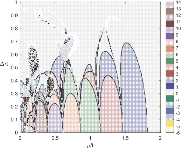
Our main result is the phase diagram shown in Fig. 2, where the parameter space includes substantial regions with odd Chern number. This diagram exhibits a series of quantum Hall transitions, where the Chern number jumps in steps of two, as we sweep the chemical potential keeping the pairing potential . At finite the jumps split to two “Majorana transitions” in which the Chern number changes by one. At large the system becomes topologically trivial, which we attribute to the localization of Cooper pairs in islands.
We then turn to examine the universal features of the phase diagram in Sec. III. We show that even though the system under study is very rich and complex, and depends on many parameters, its phase diagram shares many generic features with the phase diagrams of much simpler models. The fact that the SC pairing potential is staggered is found in Subsec. III.1 to be important to yield zero Chern number for large pairing potential. The universal properties are understood by considering the symmetries of such models, which depend (for a fixed external field) on two parameters, e.g., and , the analogs of and . When , a sweep of induces transitions between even Chern numbers in steps of two. Relieving the constraint on splits the transitions, and exposes regions with odd Chern numbers. As increases the Chern number decreases in unit steps until it vanishes for large , making the system topologically trivial. To elucidate these features, we study a simplified version of the 2D model in Subsec. III.2, and a generalization of Kitaev’s chain model Kitaev 2001 in Subsec. III.3. These two models yield phase diagrams which are similar to that of the full 2D model (see Figs. 7, 8).
We conclude with a discussion of the main results of the paper. We comment on possible realizations of the effective -wave pairing we have assumed here in systems with spin-orbit coupling, and ways to detect the topological phase using heat transport.
Details of the calculations are relegated to the following appendices. In Appendix A we provide additional details on the numerical approach used to find the ground-state phase configuration. In Appendix B we elaborate on the geometrical properties of the superlattice. In Appendix C we review the method used to calculate the Chern number in real space. In Appendix D we present several additional numerical results in the 2D system to support our main results.
II Analysis of the system
II.1 Model
We introduce the following tight-binding Hamiltonian for single-species fermions on a two-dimensional square lattice, with superimposed SC islands:
| (1) | ||||
Here are creation and annihilation operators of fermions in the lattice site labelled by , whose location is where is the lattice constant; is the chemical potential; is the hopping amplitude between nearest-neighboring sites; is the flux per unit plaquette, which enters the Hamiltonian via the Peierls substitution Peierls 1933 using the Landau gauge ; is the magnitude of the induced superconducting pairing potential; and is the phase of the superconducting order parameter in the island, which is approximately constant inside the island.
The Hamiltonian can be brought to the Bogoliuobv-de-Gennes (BdG) form by defining the Nambu spinor
| (2) |
and writing
| (3) |
where corresponds to the normal terms and corresponds to the SC terms. has particle-hole symmetry with , where is a Pauli matrix acting in particle-hole space and is complex conjugation. The magnetic field and the chiral -wave pairing terms break time-reversal symmetry , placing in symmetry class D with a topological invariantAltland and Zirnbauer 1997; Schnyder et al. 2008; Kitaev 2009.
In the Hamiltonian Eq. (1), the phases are treated as parameters. In reality, due to the interaction between the SC and the magnetic field, the ground state configuration of these phases should be determined in a self-consistent way. This can be done numerically, as elaborated in Appendix A. Due to the computational complexity of this method, we employed a simpler, approximate way to obtain the ground state phase configuration. We drawing an analogy between the current system and the two-dimensional frustrated XY model Jos 2013 – a classical theory of spins with a nearest-neighbor exchange interaction in the presence of a gauge field. Our model is composed of an array of Josephson junctions, and therefore, upon integrating out the fermionic degrees of freedom, the low-energy effective theory for the bosonic SC phases has the same symmetry properties as the frustrated XY model. The effective flux per SC plaquette is related to the actual flux per plaquette by geometric factors (see Appendix B for elaboration); concretely, for the geometry of Fig. 1. We therefore substitute the known ground state of the frustrated XY model Halsey 1985 with flux as the phase configuration of our system.
II.2 Chern number
Having established the ground state configuration, we shall henceforth treat the phases in Eq. (1) as fixed parameters and study the properties of the resulting Hamiltonian. A direct way to classify the topological properties of the system is calculating the topological invariant – the Chern number Altland and Zirnbauer 1997; Schnyder et al. 2008; Kitaev 2009. Upon casting the Hamiltonian in BdG form, the Chern number counts the number of chiral Majorana modes at the edge of the sample; an odd Chern number therefore corresponds to an unpaired chiral Majorana edge mode, which is the hallmark of topological superconductivity.
The Chern number may be calculated in momentum space Fukui et al. 2005 or in real space Yi-Fu et al. 2013; Loring and Hastings 2011. In this work we used a real-space calculation, since it is computationally more efficient and numerically robust (the details of the real-space calculation are explained in Appendix C). In particular, since the SC phases vary in space, going to momentum space is not very beneficial. All numerical calculation schemes are prone to finite size or resolution effects; we minimized these by using large enough systems such that in the absence of superconductivity (i.e. ) we obtained the known Chern numbers for the original Hofstadter model Thouless et al. 1982. We then scanned the parameter space by varying and ( is held constant, fixing the energy scale), and calculated the Chern number for each set of parameters. The resulting phase diagram for is shown in Fig. 2.

Several important features appear in the phase diagram Fig. 2. At we recover the original Hofstadter model, which gives a series of two-fold transitions of the Chern number as a function of . Recall that in the BdG form, the Chern number counts the number of Majorana edge modes, so a Chern number in the Hofstadter model becomes a BdG Chern number . The region of interest is intermediate , where a topological phase (odd Chern number) is stabilized in large areas of the parameter space, making it robust to small fluctuations in the parameters.
At large the Chern number tends to zero. The reason for this is the islands structure, namely that the SC covering is partial. For large , such a structure gives rise to localized pairs which only realize a topologically trivial phase. This argument is further supported in Subsec. III.1, where we study the effect of SC staggering analytically.
In order to complement the Chern number phase diagram we examined the energy gap as a function of and (see Fig. 10 in Appendix D), and found that near and at finite the system becomes gapless. This is because for and the system undergoes a transition of a large Chern number difference, resulting in a very small gap. Finite then mixes the states near , resulting in a gapless state. Notice that the Chern number is ill-defined in such a gapless state, so the area of the phase diagram close to is unreliable. The method we used to calculate the Chern number always yields and integer, as the system is finite so a gap always exists; however, this integer number has no real physical meaning. Therefore, in Fig. 2 we shade regions where the energy gap is smaller than the finite-size level spacing, estimated by the tight-binding bandwidth divided by the total number of sites. For completeness we show the Chern numbers of these regions in the phase diagram, although the true behavior there is metallic.

(a)
(b)
II.3 Robustness to flux
We now turn to test the dependence of the above results on the magnetic flux threaded through the system. Up to this point the flux was flux quantum per SC plaquette; we shall now examine two additional test cases, and (corresponding to and respectively), which give rise to simple enough unit cells that allow numerical investigations. The Chern number phase diagrams for these two values of the flux are shown in Fig. 3.
These phase diagrams are similar to the one obtained for (see Fig. 2). The effect of small – splitting of the two-fold transitions – persists. The effect of very large – destroying the topological phase – persists as well. The specifics do depend on the flux; in particular, the number of different phases at varies. Nevertheless, the general behavior appears to be flux-independent.
Remarkably, it seems that regardless of , substantial areas of odd Chern number are formed in the parameter space at intermediate values of . We have shown this behavior for three values of . The generic pattern we observed suggests that by tuning and , a topological phase can be stabilized for various values of .
III Universality of the phase diagram
Having calculated the phase diagrams in the previous section, we next wish to understand their generic properties. Some details vary between different values of , for example the shape of the boundary between different topological phases, the value of the gaps and the available Chern numbers of the phase diagram are not identical (see Sec. II and Figs. 2, 3). However, we find three features appearing in all cases: (i) For large pairing potential the system always becomes trivial. (ii) For the Chern numbers are even; as we change , two-fold jumps of the Chern number occur at the transitions between the phases. (iii) As we increase for fixed , successive transitions occur with mostly a reduction, and sometimes an increase, of the Chern number by one in each transition, until we reach the trivial phase with zero Chern number.
Motivated by these observations, we argue in this section that these features are universal and are shared also by other models with staggered . To demonstrate this, we analyze simplified models in both one and two dimensions that can be treated semi-analytically.
We first show that when turning off the magnetic flux in the islands model, the system becomes topologically trivial for large . We attribute this feature to localization of the Cooper pairs in regions with large pairing potential. We show that in a simplified model of the 2D system that includes the magnetic flux, where the SC phase configuration can be approximately derived, the universal features appear in the phase diagram.
The observation regarding localization of Cooper pairs applies also in one dimension, as we show analytically. This is demonstrated by analyzing a generalized one-dimensional Kitaev model with staggered pairing potential. To obtain a system with large Chern numbers in 1D, we cascade several of these staggered Kitaev chains. The resulting system is still one dimensional, as the number of chains is kept finite. The system belongs to symmetry class BDI, which means it possesses a topological invariant Kitaev 2009; Altland and Zirnbauer 1997; Schnyder et al. 2008; Fulga et al. 2012, just like the two-dimensional class D system we studied in Sec. II. We use this analogy to engineer a system with the same pattern of topological transitions as the full 2D system, by judiciously controlling the coupling between the Kitaev chains.
III.1 The effect of staggered SC
We consider a generalization of Kitaev’s chain model Kitaev 2001, which is described by the Hamiltonian
| (4) | ||||
where creates a single-species fermion at the site of the 1D lattice, is the chemical potential, is the (real) nearest-neighbor hopping amplitude, and is the SC -wave pairing potential between sites and . When is uniform, i.e. for all , the model Kitaev 2001 supports a topological phase with Majorana end modes for for any .
Consider now a staggered SC version of this model, where the pairing potential takes the values for odd and for even , as illustrated in Fig. 4(a). In momentum space, this modulation corresponds to an enlarged unit cell:
| (5) |
with
| (6a) | |||
| (6b) |
(we take the lattice constant to be unity). By analyzing the Pfaffian Kitaev 2001 of the Hamitlonian at we find that the topological phase appears for , see the ellipse in Fig. 4(b). This means that SC staggering limits the range of values for which the topological phase survives, reminiscent of the result obtained for the original 2D system. Indeed, this staggered SC configuration can be thought of as the 1D analog of the SC islands configuration we studied in the 2D case. The above result is in sharp contrast with the uniform SC case, where the phase boundaries do not depend on , provided it is non-zero.

In order to further establish the effect of a staggered SC, we also studied a simple 2D model where a similar phenomenon occurs. Consider the model on a square lattice where the SC only exists in islands as illustrated in Fig. 5(a). This is a simplification of the model we started with to the case of zero magnetic flux. For simplicity we choose each island to contain four sites (two along the direction and two along the direction). The topological properties of the system may then be analyzed by the Pfaffian of the Hamiltonian at the time-reversal invariant momenta . The phase diagram for this model is shown in Fig. 5(b), and it exhibits similar features to those of the 1D model. In particular, the range of supporting the topological phase is limited, unlike the uniform case. We have further verified that in order to get this effect, it is enough for to be staggered in any way – islands, stripes, or any other staggered patterns.

III.2 Semi-analytical 2D model
Having established the importance of a staggered , we now introduce a 2D model with magnetic flux which can be understood almost entirely from analytical considerations. We consider a system of coupled SC stripes, with a constant perpendicular magnetic field, see Fig. 6. The virtue of this model is that in the strongly anisotropic limit, where the stripes can be treated independently, we can analytically determine the ground-state SC phases.
The Hamiltonian takes the form
| (7) | ||||
The stripe lies at . The Peierls phase in the Landau gauge is . In the ground state, the gauge-invariant phase difference between every two SC bonds is zero Tinkham 1996, yielding
| (8) |
The phases reside at half-integer and integer (they connect two adjacent sites along ), and vice versa for . Therefore, in our gauge choice, a reasonable configuration is given by
| (9a) | |||
| (9b) |
Unlike the more sophisticated model studied in Sec. II, here the SC phase configuration is known. It is indeed an approximation – each stripe is treated independently of the others – but at least in the limit it is sensible. Determining the phase configuration correctly is of paramount importance: The phase diagram, and in particular the topological regions, are extremely sensitive to the SC phases (this is also demonstrated in Appendix D for the full model).
Armed with the phase configuration, we are in a position to analyze the Chern number, just as was done in Sec. II. The topological phase diagram for this model, as a function of the chemical potential and the pairing potential , is shown in Fig. 7. The phase diagram shares the important features mentioned in Subsec. II.2 with the phase diagrams of the full model (see Figs. 2, 3). In particular, it displays the crossover from the Hofstadter transitions at to the localized superconducting state at large , passing through a series of topological phases at intermediate .
The stripes structure, chosen here for its simplicity, is not special. We tested two additional variants of this semi-analytical 2D model: one where the SC stripes are replaced by SC islands, and one where the flux is only threaded in the normal regions between the SC stripes. We have also corroborated the results by applying different magnetic fluxes. The phase diagrams in all of these variants are similar, and most importantly they all share the features we refer to as universal.

III.3 Stacking several staggered Kitaev chains
Let us now turn our attention to 1D. Using the staggered Kitaev chain Eq. (5) with as a building block, we present a way to construct a phase diagram similar to the ones of the full 2D model shown in Sec. II. This is achieved by stacking staggered Kitaev chains, each having a different hopping parameter . In the absence of coupling between the chains, we get independent Chern number transitions at the values appropriate for each () and . Since we want to mimic the behavior of the full 2D system, we take an even number of chains and choose their hopping parameters to be pairwise equal, i.e. . This choice guarantees that in the absence of inter-chain coupling, the Chern number may only change by an even number at each transition.
Next, we introduce normal (non-SC) coupling of strength between neighboring chains. The role of this coupling is similar to that of in the 2D case: when turned on, it splits the two-fold Chern number transitions into single transitions, where the Chern number changes by . At large or large , the Chern number vanishes due to the SC staggering. Qualitatively, we infer that this construction reproduces the universal features we mentioned before.
In order to make the phase diagram of this model even more similar to that of the original 2D system, we perform a slight modification to . A single staggered chain with undergoes a transition of the Chern number from to at . Thus, our coupled system undergoes a transition from to at without passing at zero Chern number. Let us then choose , where is the bare coupling strength and is a small constant. This way, at the actual coupling becomes strong, thus driving the Chern number to zero. This transformation, which can be seen as a redefinition of the axes, gives rise to the phase diagram shown in Fig. 8. The resulting phase diagram is similar to the 2D phase diagrams shown in Figs. 2, 3, 7. We therefore conclude that this simple 1D model captures most of the generic features of the complicated 2D models. This observation supports the notion of universality in the phase diagrams, which applies to systems related by dimensionality and symmetry properties: class D in 2D and class BDI in 1D.

IV Discussion
In this paper, we studied the orbital effects of a magnetic field on the topological properties of the SC. Motivated by relevant experiments, we focused on a model of SC islands arranged in a square lattice. After determining the ground state configuration of the SC, we derived the topological phase diagram for different values of the magnetic flux (see Figs. 2, 3).
The tunable parameters in our model are the magnetic flux , the chemical potential , and the strength of the induced SC pairing potential . Our results suggest that for general values of the flux, it is possible to tune into a topological phase supporting Majorana edge modes by varying and . The regions in space supporting the topological phase are substantial, so the parameters do not have to be extremely fine-tuned.
Experimental detection of the Majorana edge modes can be done by interference Stern and Halperin 2006; Bonderson et al. 2006; Nilsson et al. 2008. In addition, these Majorana modes can be detected by measuring the heat conductivity, which is expected to be a half-integer multiple of in the presence of a chiral Majorana edge mode Banerjee et al. 2018. We also note that in the model we analyzed, the islands are connected by few sites, without any normal regions between them. The universality of the phase diagram we found suggests that the inclusion of normal regions between the islands, which exist in several experimental realizations, may not alter the main features of the phase diagram.
Our model should be understood as an effective description of a more complicated physical system. We assumed the existence of an induced -wave pairing potential and single-species fermions. One can take a more microscopic approach and study spinful electrons with spin-orbit coupling, proximity coupled to an -wave SC with an applied Zeeman field, which can give rise to induced -wave pairing. It is also possible (at least numerically) to account for disorder, which is not expected to have a drastic effect on the results provided it is smaller than the energy gap. Likewise, our zero-temperature study may be generalized to finite temperatures, but as long as the SC gap is larger than the temperature, our results are expected to hold qualitatively.
We also studied simplified, analytically solvable models in 1D and 2D which share common features with the original 2D model. We found that the islands structure (and more generally the staggering of the SC pairing potential) has a profound implication on the topological phase diagram: Pair localization at large drives the system away from the topological phase. We showed that a model consisting of coupled staggered 1D Kitaev-like chains exhibits a topological phase diagram which greatly resembles those of the original 2D model (see Fig. 8). These findings suggest that several features of the phase diagram are shared by many models. The results shed light on those obtained for the original model, which relied mainly on numerics.
This notion of universality may also be viewed from a general mathematical perspective. Consider a model with two tunable parameters and , such that at the Chern number has to be even. Assume further that at large and the Chern number has to vanish, and that at the generic behavior is one-fold Chern number transitions. Under such settings, it is almost impossible to construct a phase diagram which is topologically distinct from those shown in Figs. 2, 3, 7, 8. We conclude that the phase diagrams we found have universal features and may appear under very general settings.
Acknowledgements
We are grateful to Eran Sagi for participating in the early stages of this project. We are thankful for discussions with B. I. Halperin. The research was supported by the European Union’s Horizon 2020 research and innovation programme grant agreement LEGOTOP No 788715, the DFG (CRC/Transregio 183, EI 519/7- 1), the Israel Science Foundation (ISF) and the Binational Science Foundation (BSF).
Appendix A Determining the Ground State
The Hamiltonian Eq. (1) depends on all the islands’ phases . Here we describe a direct numerical method of finding the ground state configuration of .
The system possesses a global symmetry, i.e., the transformation for all leaves the energy invariant for constant . Therefore, without loss of generality we set one of the phases, say , to zero. The Hamiltonian thus depends on phases.
When writing the Hamiltonian in BdG form as in Eq. (3), the many-body ground state energy is given by the sum of all negative eigenvalues of , i.e.
| (10) |
where is the step function and are the eigenvalues of . is a function of , and our goal is to find the configuration of that minimizes it.
We carried out the optimization in real space, using a finite system with periodic boundary conditions. We used the optimization algorithm “interior-point” Karmarkar 1984; Forsgren et al. 2002. In order to increase the probability of finding the global minimum point, we used many random initial conditions for . We compared this numerical method and the known frustrated XY ground states for several fluxes, and found that the configurations are qualitatively similar. We note that the optimization is sensitive to the initial conditions, and many local minima exist, so multiple runs are necessary in order to get a good agreement with the results of the frustrated XY model. The numerical optimization shows that the ground-state configurations of the frustrated XY model are at least local minima of our model.
Appendix B Geometric relation between and
Let us denote the number of lattice sites per dimension per island by where is the spatial dimension, and the number of plaquettes separating adjacent islands per dimension by (see Fig. 9). Then, the area of a superlattice unit cell is , and the area of a magnetic unit cell is . The flux per magnetic plaquette is and the flux per superlattice unit cell is (see Fig. 1). The factor of comes from the fact that the relevant flux quantum for the superconductor is that of Cooper pairs. The relation between and is thus
| (11) |
In the current study we used and , yielding the relation . The largest value of we investigated is and therefore the largest value of is , so the approximation of a constant phase inside each island is reasonable.
Appendix C Real space calculation of the Chern number
Here we review the method devised in Refs. Yi-Fu et al. 2013; Loring and Hastings 2011 of calculating the Chern number from the real space Hamiltonian. Consider a 2D lattice with unit cells, and denote their positions by where are integers. Let us define twisted periodic boundary conditions by
| (12) |
where are the single-particle wavefunctions ( where is the number of electrons), which are vectors in the space of inner degrees of freedom. The many-body ground-state wavefunction is the Slater determinant of the single-particle wavefunctions of the occupied states, and the Chern number is given by
| (13) |
where is the torus .
Going to momentum space, we denote by the Fourier components of . The twisted boundary conditions dictate the allowed momenta,
| (14) |
Denoting , we note that the many-body wavefunction in momentum space is just the Slater determinant of . Thus, upon substituting (here ) we obtain an equation for the Chern number:
| (15) |
where is the rectangle . Using Stokes’ theorem, the above expression can be written as a winding number along the boundary ,
| (16) |
Next, we divide into small line segments and replace the derivatives and integral by their discrete counterparts to obtain
| (17) |
where are the coupling matrices and are the endpoints of the small line segments.
If , i.e., we consider a sufficiently large system, it is enough to take , corresponding to (i.e. just the four corners of ). In this case we only need to deal with quantities calculated for periodic boundary conditions. Transforming the coupling matrices back to real space for we obtain
| (18) |
We may thus define the matrix , diagonalize it to obtain the eigenvalues , and calculate the Chern number:
| (19) |
If the Hamiltonian is written in the BdG form, this method yields the BdG Chern number .
Appendix D Additional numerical results in the 2D system
We now present several additional results in the full 2D system, described by the Hamiltonian Eq. (3). These results were obtained numerically, and they support the arguments given in Sec. II of the main text: the vanishing of the energy gap near and the strong dependence of the topological phase diagram on the SC phases.
Fig. 10 shows the energy gap as a function of the model’s parameters for . Compared with the phase diagram Fig. 2, it is evident that the topological phases are gapped. In addition, this map makes the transitions of the Chern number transparent – they are accompanied by a closing of the energy gap.

Fig. 11 shows the Chern number phase diagram for , in the case where the SC phases are uniform, i.e. for all . This phase configuration is not the ground state due to the presence of the magnetic field. Though it resembles the true phase diagram Fig. 2 in its general shape, this phase diagram does not support odd Chern number phases. This observation emphasizes the role of the SC phases and the vortices induced by the magnetic field.
References
- Alicea (2012) J. Alicea, Reports on Progress in Physics 75, 076501 (2012).
- Bernevig and Hughes (2013) B. A. Bernevig and T. L. Hughes, Topological Insulators and Topological Superconductors (Princeton university press, 2013).
- Nayak et al. (2008) C. Nayak, S. H. Simon, A. Stern, M. Freedman, and S. Das Sarma, Reviews of Modern Physics 80, 1083 (2008).
- Sau et al. (2010) J. D. Sau, R. M. Lutchyn, S. Tewari, and S. Das Sarma, Physical Review Letters 104, 040502 (2010).
- Palacio-Morales et al. (2019) A. Palacio-Morales, E. Mascot, S. Cocklin, H. Kim, S. Rachel, D. K. Morr, and R. Wiesendanger, Science Advances 5, eaav6600 (2019).
- Lutchyn et al. (2010) R. M. Lutchyn, J. D. Sau, and S. Das Sarma, Physical Review Letters 105, 077001 (2010).
- Oreg et al. (2010) Y. Oreg, G. Refael, and F. von Oppen, Physical Review Letters 105, 177002 (2010).
- Albuquerque et al. (2008) A. F. Albuquerque, H. G. Katzgraber, M. Troyer, and G. Blatter, Physical Review B 78, 014503 (2008).
- Alicea (2010) J. Alicea, Physical Review B 81, 125318 (2010).
- Fu and Kane (2008) L. Fu and C. L. Kane, Physical Review Letters 100, 096407 (2008).
- Qi et al. (2010) X.-L. Qi, T. L. Hughes, and S.-C. Zhang, Physical Review B 82, 184516 (2010).
- (12) Full shell systems are an exception; see Ref. Lutchyn et al. 2018.
- v. Klitzing et al. (1980) K. v. Klitzing, G. Dorda, and M. Pepper, Physical Review Letters 45, 494 (1980).
- Stern (2008) A. Stern, Annals of Physics January Special Issue 2008, 323, 204 (2008).
- Girvin (1999) S. M. Girvin, in Aspects Topologiques de La Physique En Basse Dimension. Topological Aspects of Low Dimensional Systems, Les Houches - Ecole d’Ete de Physique Theorique, edited by A. Comtet, T. Jolicœur, S. Ouvry, and F. David (Springer Berlin Heidelberg, 1999) pp. 53–175.
- Harper (1955) P. G. Harper, Proceedings of the Physical Society. Section A 68, 874 (1955).
- Hofstadter (1976) D. R. Hofstadter, Physical Review B 14, 2239 (1976).
- Bøttcher et al. (2018) C. G. L. Bøttcher, F. Nichele, M. Kjaergaard, H. J. Suominen, J. Shabani, C. J. Palmstrøm, and C. M. Marcus, Nature Physics 14, 1138 (2018).
- Aleiner et al. (2002) I. L. Aleiner, P. W. Brouwer, and L. I. Glazman, Physics Reports 358, 309 (2002).
- Jos (2013) J. V. Jos, 40 Years of Berezinskii-Kosterlitz-Thouless Theory (World Scientific, 2013).
- (21) They can be eliminated if the magnetic field is applied in-plane and strong Dresselhaus spin-orbit coupling (like in (111) InSb samples Alicea 2010) is present Dresselhaus 1955; Levine et al. 2017.
- Altland and Zirnbauer (1997) A. Altland and M. R. Zirnbauer, Physical Review B 55, 1142 (1997).
- Schnyder et al. (2008) A. P. Schnyder, S. Ryu, A. Furusaki, and A. W. W. Ludwig, Physical Review B 78, 195125 (2008).
- Kitaev (2009) A. Kitaev, AIP Conference Proceedings 1134, 22 (2009).
- Kitaev (2001) A. Y. Kitaev, Physics-Uspekhi 44, 131 (2001).
- Peierls (1933) R. Peierls, Zeitschrift für Physik 80, 763 (1933).
- Halsey (1985) T. C. Halsey, Physical Review B 31, 5728 (1985).
- Fukui et al. (2005) T. Fukui, Y. Hatsugai, and H. Suzuki, Journal of the Physical Society of Japan 74, 1674 (2005).
- Yi-Fu et al. (2013) Z. Yi-Fu, Y. Yun-You, J. Yan, S. Li, S. Rui, S. Dong-Ning, and X. Ding-Yu, Chinese Physics B 22, 117312 (2013).
- Loring and Hastings (2011) T. A. Loring and M. B. Hastings, EPL (Europhysics Letters) 92, 67004 (2011).
- Thouless et al. (1982) D. J. Thouless, M. Kohmoto, M. P. Nightingale, and M. den Nijs, Physical Review Letters 49, 405 (1982).
- Fulga et al. (2012) I. C. Fulga, F. Hassler, and A. R. Akhmerov, Physical Review B 85, 165409 (2012).
- Tinkham (1996) M. Tinkham, Introduction to Superconductivity, 2nd ed., International Series in Pure and Applied Physics (McGraw-Hill, New York, 1996).
- Stern and Halperin (2006) A. Stern and B. I. Halperin, Physical Review Letters 96, 016802 (2006).
- Bonderson et al. (2006) P. Bonderson, A. Kitaev, and K. Shtengel, Physical Review Letters 96, 016803 (2006).
- Nilsson et al. (2008) J. Nilsson, A. R. Akhmerov, and C. W. J. Beenakker, Physical Review Letters 101, 120403 (2008).
- Banerjee et al. (2018) M. Banerjee, M. Heiblum, V. Umansky, D. E. Feldman, Y. Oreg, and A. Stern, Nature 559, 205 (2018).
- Karmarkar (1984) N. Karmarkar, in Proceedings of the Sixteenth Annual ACM Symposium on Theory of Computing, STOC ’84 (ACM, New York, NY, USA, 1984) pp. 302–311.
- Forsgren et al. (2002) A. Forsgren, P. E. Gill, and M. H. Wright, SIAM review 44, 525 (2002).
- Lutchyn et al. (2018) R. M. Lutchyn, G. W. Winkler, B. van Heck, T. Karzig, K. Flensberg, L. I. Glazman, and C. Nayak, arXiv:1809.05512 [cond-mat] (2018), arXiv:1809.05512 [cond-mat] .
- Dresselhaus (1955) G. Dresselhaus, Physical Review 100, 580 (1955).
- Levine et al. (2017) Y. Levine, A. Haim, and Y. Oreg, Physical Review B 96, 165147 (2017).