Multi-scale Domain-adversarial Multiple-instance CNN for Cancer Subtype Classification with Unannotated Histopathological Images

Noriaki Hashimoto Daisuke Fukushima Ryoichi Koga Yusuke Takagi Kaho Ko Kei Kohno Masato Nakaguro Shigeo Nakamura Hidekata Hontani Ichiro Takeuchi Affiliation: Nagoya Institute of Technology, Nagoya University Hospital, RIKEN

Abstract

We propose a new method for cancer subtype classification from histopathological images, which can automatically detect tumor-specific features in a given whole slide image (WSI). The cancer subtype should be classified by referring to a WSI, i.e., a large-sized image (typically 40,000 $\times$ 40,000 pixels) of an entire pathological tissue slide, which consists of cancer and non-cancer portions. One difficulty arises from the high cost associated with annotating tumor regions in WSIs. Furthermore, both global and local image features must be extracted from the WSI by changing the magnifications of the image. In addition, the image features should be stably detected against the differences of staining conditions among the hospitals/specimens. In this paper, we develop a new CNN-based cancer subtype classification method by effectively combining multiple-instance, domain adversarial, and multi-scale learning frameworks in order to overcome these practical difficulties. When the proposed method was applied to malignant lymphoma subtype classifications of 196 cases collected from multiple hospitals, the classification performance was significantly better than the standard CNN or other conventional methods, and the accuracy compared favorably with that of standard pathologists.

⁰⁰ 0 ^$\dagger$N.H. and D.F. contributed equally. ^*Correspondence to I.T. (e-mail: takeuchi.ichiro@nitech.ac.jp).

1 Introduction

In this study, we propose a novel convolutional neural network (CNN)-based method for cancer subtype classification by using digital pathological images of hematoxylin-and-eosin (H&E) stained tissue specimens as inputs. Since a whole slide image (WSI) obtained by digitizing an entire pathological tissue slide is too large to feed into a CNN krizhevsky2012imagenet; simonyan2014very; he2016deep; chollet2017xception, it is common to extract a large number of patches from the WSI cirecsan2013mitosis; cruz2014automatic; mousavi2015automated; xu2015deep; hou2016patch; wang2016deep; bejnordi2017diagnostic; xu2017large; bandi2018detection; graham2018classification. If it can be known whether each patch is a tumor region or not, the CNN can be trained by using each patch as a labeled training instance. However, the cost to annotate each of a large number of patch labels is too high. When patch label annotation is not available, cancer subtype classification tasks are challenging in the following three respects.

The first difficulty is that tumor and non-tumor regions are mixed in a WSI. Therefore, when pathologists actually conduct subtype classification, it is necessary to find out which part of the slide contains the tumor region, and perform subtype classification based on the features of the tumor region. The second practical difficulty is that staining conditions vary greatly depending on the specimen conditions and the hospital from which the specimen was taken. Therefore, pathologists perform tumor region identification and subtype classification by carefully considering the different staining conditions. The last difficulty is that different features of tissues are observed when the magnification of the pathological image is changed. Pathologists conduct diagnosis by changing the magnification of a microscope repeatedly to find out various features of the tissues.

In order to develop a practical CNN-based subtype classification system, our main idea is to introduce mechanisms that mimic these pathologist’s actual practices. To address the above three difficulties simultaneously, we effectively combine multiple instance learning (MIL), domain adversarial (DA) normalization, and multi-scale (MS) learning techniques. Although each of these techniques has been studied in the literatures, we demonstrate that their effective and careful combination enables us to develop a CNN-based system that performs significantly better than the standard CNN or other conventional methods.

We applied the proposed method to malignant lymphoma subtype classifications of 196 cases collected from 80 hospitals, and demonstrated that the accuracy of the proposed method compared favorably with standard pathologists. It was also confirmed that the proposed method not only performed better than conventional methods, but also performed subtype classification in a similar way to pathologists in the sense that the method correctly paid attention to tumor regions in images of various different scales.

The main contributions of our study are as follows. First, we developed a novel CNN-based digital pathology image classification method by effectively combining MIL, DA and MS approaches. Second, we applied the proposed method to malignant lymphoma classification tasks with 196 WSIs of H&E stained histological tissue slides, collected for the purpose of consultation by an expert pathologist on malignant lymphoma. Finally, as a result of confirmation by immunostaining in the above malignant lymphoma subtype classification tasks, it was confirmed that the proposed method performed subtype classification by correctly paying attention to the true tumor regions from images at various different scales of magnification.

2 Preliminaries

Here we present our problem setup and three related techniques that are incorporated into the proposed method in the next section. In this paper, we use the following notations. For any natural number $N$ , we define $[N]:=\{1,\ldots,N\}$ . We call a vector for which the elements are non-negative and sum-to-one a probability vector. Given two probability vectors $p,q$ , ${\mathcal{L}}(p,q)$ represents their cross entropy.

2.1 Problem setup

Consider a training set for a binary pathological image classification problem obtained from $N$ patients. We denote the training set as $\{(\mathbb{X}_{n},\mathbb{Y}_{n})\}_{n=1}^{N}$ , where $\mathbb{X}_{n}$ is the whole slide image (WSI) and $\mathbb{Y}_{n}$ is the two-dimensional class label one-hot vector of the $n^{\rm th}$ patient for $n\in[N]$ . We also define a set of $N$ -dimensional vectors $\{\mathbb{D}_{n}\}_{n=1}^{N}$ for which the $n^{\rm th}$ element is one and the others are zero. Since each WSI is too huge to directly feed into a CNN, a patch-based approach is usually employed. In this paper, we consider patches with $224\times 224$ pixels.

In cancer pathology, since tumor and non-tumor regions are mixed, not all patches from a positive-class slide contain positive class-specific (tumor) information. Thus, we borrow an idea from multiple instance learning (MIL) (the detail of MIL will be described in § 2.2). Specifically, we consider a group of patches, and assume that each group from a positive class slide contains at least a few patches having positive class-specific information, whereas each group from a negative class slide does not contain any patches having positive-class specific information. Furthermore, when pathologists diagnose patients, they observe the glass slide at multiple different scales. To mimic this, we consider patches with multiple different scales.

We denote the groups of patches at different scales as follows. We use the notation $s\in[S]$ to indicate the index of scales (e.g., if scales 10x and 20x are considered, $S=2$ ). The set of groups (called bags in MIL framework) in the $n^{\rm th}$ WSI is denoted by ${\mathcal{B}}_{n}$ for $n\in[N]$ . Then, each group (bag) $b\in{\mathcal{B}}_{n}$ is characterized by a set of patches (called instances in the MIL framework) ${\mathcal{I}}_{b}^{(s)}$ for $b\in{\mathcal{B}}_{n}$ and $s\in[S]$ , where the superscript ^(s) indicates that these patches are taken from scale $s$ . Figure 1 illustrates the notions of a WSI, groups (bags), patches (instances), and scales.

Refer to caption — Figure 1: A brief illustration of the notions of a WSI, bags, instances (patches), and scales. A large number of $224\times 224$ -pixel image patches are extracted from an entire WSI at multiple different scales. In the problem setup considered in this paper, instance class labels are not observed, but the class labels for groups of instances called bags are observed. It is important to note that each bag contains patches taken at multiple different scales. This enables us to detect multiple regions of interest from multiple different scale images.

2.2 Multiple instance learning (MIL)

Multiple-instance learning (MIL) is a type of weakly supervised learning problem, where instance labels are not observed but labels for groups of instances called bags are observed. In the binary classification setting, a positive label is assigned to a bag if the bag contains at least one positive instance, while a negative label is assigned to a bag if the bag only contains negative instances. Figure 2 illustrates MIL for a binary classification problem. Various models and learning algorithms for MIL have been studied in the literatures dietterich1997solving; maron1998framework; zhou2002neural; andrews2003support; li2012efficient; chen2013multi; wu2015deep.

MIL has been successfully applied to classification problems with histopathological images cosatto2013automated; das2018multiple; ilse2018attention; couture2018multiple; sudharshan2019multiple; campanella2019clinical. For example, for binary classification of malignant and benign patients, WSIs for malignant patients contain both malignant and benign patches, while WSIs for benign patients only contain benign patches. If we regard the WSIs for malignant/benign patients as positive/negative bags and malignant/benign patches as positive/negative instances, respectively, the above binary classification problem can be interpreted as an MIL problem. The MIL framework is useful in histopathological image classification when no annotation is made for each extracted patch. Our main idea in this paper is to use MIL framework in order to automatically identify multiple regions of interest at multiple different scales.

Figure 2: Explanation of MIL. Positive bags are generated from WSIs with positive subtype labels and negative bags are generated from WSIs with negative subtype labels. Only the image patches of class-specific regions, such as tumors in positive-class WSIs, are regarded as positive instances.

2.3 Domain-adversarial neural network

Slide-wise differences in staining conditions, as illustrated in Fig. 3, highly degrade the classification accuracy. To overcome this difficulty, appropriate pre-processing such as color normalization reinhard2001color; macenko2009method; khan2014nonlinear; bejnordi2015stain; zanjani2018histopathology or color augmentation lafarge2017domain; rakhlin2018deep would be required. Color normalization adjusts the color of input images to the target color distribution. Color augmentation suppresses the effect of outlying colors by generating augmented images while slightly changing the color of an original image.

Domain-adversarial (DA) ganin2016domain training has been proposed to ignore the differences among training instances that do not contribute to the classification task. In the histopathological image classification setting, Lafarge et al. lafarge2017domain introduced a DA training approach, and demonstrated that it was superior to color augmentation, stain normalization, and their combination. In the proposed method, we use a DA training approach within the MIL framework for histopathological image classification by regarding each patient as an individual domain so that the staining condition of each patient’s slide can effectively be ignored.

2.4 Multi-scale pathology image analysis

Pathologists observe different features at different scales of magnification. For example, global tissue structure and detailed shapes of nuclei can be seen at low and high scales of magnification, respectively. Although most of the existing studies on histopathological image analysis use a fixed single scale, some studies use multiple scales bejnordi2015multi; gao2016multi; wetteland2019multiscale; tokunaga2019adaptive.

When multi-scale images are available in histopathological image analysis, a common approach is to use them hierarchically from low resolution to high resolution. Namely, a low-resolution image is first used to detect regions of interest, and then high-resolution images of the detected regions are used for further detailed analysis. Another approach is to automatically select the appropriate scale from the image itself. For example, Tokunaga et al. tokunaga2019adaptive employed a mixture-of-expert network, where each expert was trained with images of different scale, and the gating network selected which expert should be used for segmentation.

In this study, we noted that expert pathologists conduct diagnosis by changing the magnification of a microscope repeatedly to find out various features of the tissues. This indicates that the analysis of multiple regions at multiple scales plays a significant role in subtype classification. In order to mimic this pathologists’ practice, we propose a novel method to use multiple patches at multiple different scales within the MIL framework. In contrast to the hierarchical or selective usage of multi-scale images, our approach uses multi-scale images simultaneously.

3 Proposed method

In the proposed method, the subtype of each patient is predicted based on the H&E stained WSI by summarizing the predicted class labels of the bags taken from the WSI. Specifically, given a test WSI $\mathbb{X}_{n}$ , the class label probability is simply predicted as $P(\hat{\mathbb{Y}}_{n}=1)=p_{1}/(p_{1}+p_{0})$ , where

	$\displaystyle p_{1}=\exp\left(\frac{1}{\|{\mathcal{B}}_{n}\|}\sum_{b\in{\mathcal{B}}_{n}}\log P(\hat{Y}_{b}=1)\right),$
	$\displaystyle p_{0}=\exp\left(\frac{1}{\|{\mathcal{B}}_{n}\|}\sum_{b\in{\mathcal{B}}_{n}}\log P(\hat{Y}_{b}=0)\right).$

Here, $P(\hat{Y}_{b}=1)$ and $P(\hat{Y}_{b}=0)$ are the class label probabilities of the bag $b\in{\mathcal{B}}_{n}$ .

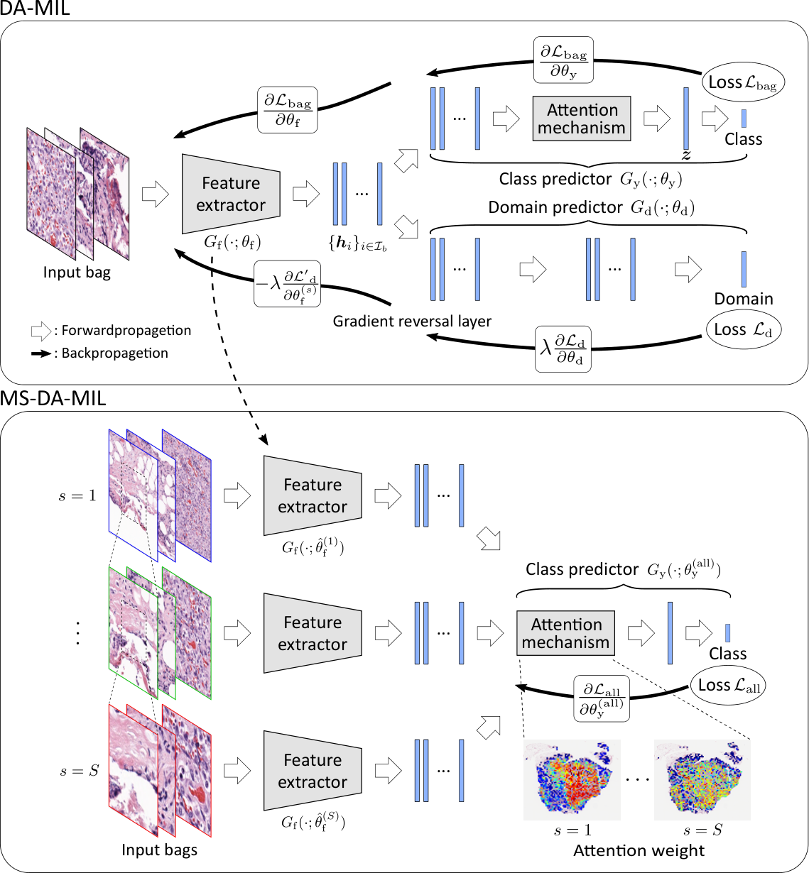
The bag’s class label probability is obtained as the output of the proposed CNN network, as depicted in Fig. 4. It consists of the following three building blocks. Feature extractor $G_{\rm{f}}:\bm{x}\mapsto\bm{h}$ is a CNN which maps a $224\times 224$ -pixel image $\bm{x}$ into a $Q$ -dimensional feature vector $\bm{h}$ . It is denoted as $\bm{h}=G_{\rm{f}}(\bm{x};\theta_{\rm{f}})$ where $\theta_{\rm{f}}$ is the set of trainable parameters. Bag class label predictor $G_{\rm{y}}:\{\bm{h}_{i}\}_{i\in{\mathcal{I}}_{b}}\mapsto P(\hat{Y}_{b})$ is an NN with an attention mechanism ilse2018attention that maps the set of feature vectors in a bag $b$ into the probabilities of the bag class label $\hat{Y}_{b}$ . $G_{\rm{y}}(\cdot;\theta_{\rm{y}})$ is characterized by a set of trainable parameters $\theta_{\rm{y}}$ , where $(\bm{V},\bm{w})\in\theta_{\rm{y}}$ are the sets of parameters for the attention network. Using $Q^{\prime}$ -dimensional feature vectors $\{\bm{h}^{\prime}_{i}\}_{i\in{\mathcal{I}}_{b}}$ generated through the fully connected layer, the attention weighted feature vector $\bm{z}\in\mathbb{R}^{Q^{\prime}}$ is obtained as $\bm{z}=\sum_{i\in{\mathcal{I}}_{b}}a_{i}\bm{h}^{\prime}_{i}$ , where each attention is defined as

\displaystyle a_{i}=\frac{\exp\left(\bm{w}^{\top}{\rm tanh}(\bm{V}\bm{h}^{\prime}_{i})\right)}{\sum_{j\in{\mathcal{I}}_{b}}\exp\left(\bm{w}^{\top}{\rm tanh}(\bm{V}\bm{h}^{\prime}_{j})\right)},i\in{\mathcal{I}}_{b}.

Domain predictor $G_{\rm{d}}:\bm{h}\mapsto P(\hat{d})$ is a simple NN that maps a feature vector $\bm{h}$ into domain label probabilities $P(\hat{d})$ . It is denoted as $G_{\rm{d}}(\bm{h};\theta_{\rm{d}})$ , where $\theta_{\rm{d}}$ is the set of trainable parameters. Training of the proposed CNN network is conducted in two stages. In the first stage, a single-scale DA-MIL network (the top one in Fig. 4) is trained to obtain the feature extractor $G_{\rm{f}}(\cdot;\theta_{\rm{f}}^{(s)})$ for each scale $s\in[S]$ . Then, in the second stage, a multi-scale DA-MIL network (the bottom one in Fig. 4) is trained by plugging the $S$ trained feature extractors into the network.

3.1 Stage1: single-scale learning

In stage 1, a single-scale DA-MIL network is trained for each scale $s\in[S]$ to predict the bag class labels where each bag only contains patches from the image of scale $s$ . Here we modified the DA regularization ganin2016domain in order to apply it to only image patches with lower attention weights of MIL. The training task of a single-scale DA-MIL network is formulated as the following minimization problem:

		$\displaystyle\left(\hat{\theta}_{\rm{f}}^{(s)},\hat{\theta}_{\rm{y}}^{(s)},\hat{\theta}_{\rm{d}}^{(s)}\right)\leftarrow\arg\min_{\theta_{\rm{f}}^{(s)},\theta_{\rm{y}}^{(s)},\theta_{\rm{d}}^{(s)}}\sum_{n=1}^{N}\sum_{b\in{\mathcal{B}}_{n}}{\mathcal{L}}(\mathbb{Y}_{n},P(\hat{Y}_{b}^{(s)}))$
		$\displaystyle-\lambda\sum_{n=1}^{N}\sum_{b\in{\mathcal{B}}_{n}}\frac{1}{\|{\mathcal{I}}_{b}^{(s)}\|}\sum_{i\in{\mathcal{I}}_{b}^{(s)}}\beta_{i}{\mathcal{L}}(\mathbb{D}_{n},G_{\rm{d}}(\bm{h}_{i};\theta_{\rm{d}}^{(s)})),$		(1)

where

	$\displaystyle P(\hat{Y}_{b}^{(s)})$	$\displaystyle=G_{\rm{y}}\left(\{G_{\rm{f}}(\bm{x}_{i};\theta_{\rm{f}}^{(s)})\}_{i\in{\mathcal{I}}_{b}^{(s)}};\theta_{\rm{y}}^{(s)}\right),$
	$\displaystyle\beta_{i}$	$\displaystyle=\max_{a_{j}}\{a_{j}\|j\in{\mathcal{I}}_{b}^{(s)}\}-a_{i}.$

In eq. (1), the first term is the loss function for bag class label prediction, while the second term is the penalty function for DA regularization, which is weighted by attentions for each instance. The loss function is simply defined by the cross entropy between the true class label and predicted class label probability. Here, the bag class label is predicted by only using instances for which the attentions are large. The DA regularization term is also defined by the cross entropy between the domain label and the predicted domain label probability. By penalizing the domain prediction capability using DA regularization, the feature extractor $G_{\rm{f}}(\cdot;\theta_{\rm{f}}^{(s)})$ for each $s\in[S]$ is trained so that the difference in staining conditions can be ignored.

3.2 Stage2: multi-scale learning

In stage 2, a multi-scale DA-MIL network is trained to predict the bag class label where each bag contains instances (patches) across different scales. The bag class label is predicted as

\displaystyle P(\hat{Y}_{b})=G_{\rm{y}}\left(\{\{G_{\rm{f}}(\bm{x}_{i};\hat{\theta}_{\rm{f}}^{(s)})\}_{i\in{\mathcal{I}}_{b}^{(s)}}\}_{s=1}^{S};\theta_{\rm{y}}^{(\rm all)}\right),

where the set of feature extractors $G_{\rm{f}}(\cdot;\hat{\theta}_{\rm{f}}^{(s)})$ , $s\in[S]$ , which were already trained in the first stage, are plugged in. The training of the set of parameters $\theta_{\rm{y}}^{(\rm all)}$ is formulated as the following minimization problem:

\displaystyle\hat{\theta}_{\rm{y}}^{(\rm all)}\leftarrow\arg\min_{\theta_{\rm{y}}^{(\rm all)}}\sum_{n=1}^{N}\sum_{b\in{\mathcal{B}}_{n}}{\mathcal{L}}(\mathbb{Y}_{n},P(\hat{Y}_{b})).

(2)

3.3 Algorithm

The algorithm of our proposed method is described in Algorithm 1. Each parameter update is conducted by using the instances (patches) in each bag as a mini-batch.

Algorithm 1 Parameter update in MS-DA-MIL training.

0: training set

\{(\mathbb{X}_{n},\mathbb{Y}_{n})\}_{n=1}^{N}

with domain label

\{\mathbb{D}_{n}\}_{n=1}^{N}

, learning rate

\eta

, domain regularization parameter

\lambda

, train epochs

M

% stage 1: train feature extractor

G_{\rm{f}}(\cdot;\theta_{\rm{f}}^{(s)})

, class predictor

G_{\rm{y}}(\cdot;\theta_{\rm{y}}^{(s)})

, domain predictor

G_{\rm{d}}(\cdot;\theta_{\rm{d}}^{(s)})

for

m=1

M

for

s=1

S

for

n=1

N

for

b=1

|\mathcal{B}_{n}|

\{\bm{h}_{i}\}_{i\in\mathcal{I}_{b}^{(s)}}\leftarrow\{G_{\rm{f}}(\bm{x}_{i};\theta_{\rm{f}}^{(s)})\}_{i\in\mathcal{I}_{b}^{(s)}}

\mathcal{L}_{\rm{bag}}\leftarrow\mathcal{L}\left(\mathbb{Y}_{n},G_{\rm{y}}(\{\bm{h}_{i}\}_{i\in\mathcal{I}_{b}^{(s)}};\theta_{\rm{y}}^{(s)})\right)

\mathcal{L}_{\rm{d}}\leftarrow\frac{1}{|\mathcal{I}_{b}^{(s)}|}\sum_{i\in\mathcal{I}_{b}^{(s)}}\mathcal{L}\left(\mathbb{D}_{n},G_{\rm{d}}(\bm{h}_{i};\theta_{\rm{d}}^{(s)})\right)

\mathcal{L^{\prime}}_{\rm{d}}\leftarrow\frac{1}{|\mathcal{I}_{b}^{(s)}|}\sum_{i\in\mathcal{I}_{b}^{(s)}}\beta_{i}\mathcal{L}\left(\mathbb{D}_{n},G_{\rm{d}}(\bm{h}_{i};\theta_{\rm{d}}^{(s)})\right)

\beta_{i}=\max_{a_{j}}\{a_{j}|j\in{\mathcal{I}}_{b}^{(s)}\}-a_{i}

\theta_{\rm{y}}^{(s)}\leftarrow\theta_{\rm{y}}^{(s)}-\eta\frac{\partial\mathcal{L}_{\rm{bag}}}{\partial\theta_{\rm{y}}^{(s)}}

\theta_{\rm{d}}^{(s)}\leftarrow\theta_{\rm{d}}^{(s)}-\eta\lambda\frac{\partial\mathcal{L}_{\rm{d}}}{\partial\theta_{\rm{d}}^{(s)}}

\theta_{\rm{f}}^{(s)}\leftarrow\theta_{\rm{f}}^{(s)}-\eta\left(\frac{\partial\mathcal{L}_{\rm{bag}}}{\partial\theta_{\rm{f}}^{(s)}}-\lambda\frac{\partial\mathcal{L^{\prime}}_{\rm{d}}}{\partial\theta_{\rm{f}}^{(s)}}\right)

end for

end for% stage 2: train class predictor

G_{\rm{y}}(\cdot;\theta_{\rm{y}}^{(\rm{all})})

for

m=1

M

for

n=1

N

for

b=1

|\mathcal{B}_{n}|

{\mathcal{L}}_{\rm all}\leftarrow{\mathcal{L}}(\mathbb{Y}_{n},P(\hat{Y}_{b}))

P(\hat{Y}_{b})=G_{\rm{y}}(\{\{G_{\rm{f}}(\bm{x}_{i};\theta_{\rm{f}}^{(s)})\}_{i\in\mathcal{I}_{b}^{(s)}}\}_{s=1}^{S};\theta_{\rm{y}}^{(\rm{all})})

\theta_{\rm{y}}^{(\rm{all})}\leftarrow\theta_{\rm{y}}^{\rm{(all)}}-\eta\frac{\partial\mathcal{L}_{\rm all}}{\partial\theta_{\rm{y}}^{\rm{(all)}}}

end for

neural network

\{\{\theta_{\rm{f}}^{(s)}\}_{s=1}^{S},\theta_{\rm{y}}^{\rm{(all)}}\}

4 Experiments

Dataset

Our experimental database of malignant lymphoma was composed of 196 clinical cases, which represented difficult lymphoma cases from 80 different institutions, and had been sent to an expert pathologist for diagnostic consultation. As malignant lymphoma has a lot of subtypes, in addition to observing an H&E stained tissue, serial sections from the same patient’s sample are immunohistochemically stained to confirm its expression patterns for final decision making. It is expected that predicting various subtypes of malignant lymphoma is quite difficult by analyzing only the H&E stained tissue images and its difficulty was not revealed. We use the cases with only five typical types of malignant lymphoma: diffuse large B-cell lymphoma (DLBCL), angioimmunoblastic T-cell lymphoma (AITL), classical Hodgkin’s lymphoma mixed cellularity (HLMC) and classical Hodgkin’s lymphoma nodular sclerosis (HLNS). In addition, DLBCL is classified into two subtypes; germinal center B-cell (GCB) and non-germinal center B-cell (non-GCB) types. In this experiment, as a first step, we perform two-class classification, which discriminates DLBCL consisting both GCB and non-GCB types from the other three non-DLBCL classes including AITL, HLMC and HLNS. In applying our proposed method to this classification problem, DLBCL and non-DLBCL are respectively defined as positive and negative classes, as explained in the previous sections. Here, the positive instance means that an instance has the capability to discriminate DLBCL from non-DLBCL, and it should be in tumor regions of DLBCL cases because non-tumor regions in DLBCL are expected to have similar features to those in non-tumor regions in non-DLBCL cases. Hence, a bag indicates a set of image patches extracted from a WSI, where positive instances represent images from tumor regions in DLBCL and negative instances represent images from non-tumor regions in DLBCL and all patches in non-DLBCL. As the total number of DLBCL cases was 98, the same number of non-DLBCL cases were selected from AITL, HLMC and HLNS cases. All glass slides of the H&E stained tissue specimens collected as mentioned above were scanned with an Aperio ScanScopeXT (Leica Biosystems, Germany) at 20x magnification (0.50 um/pixel).

Experimental setup

In the experiments, we used 10x (1.0 um/pixel) and 20x-magnification (0.50 um/pixel) images, that is, the scale parameter $S$ was set to 2. We split the dataset mentioned above into 60% training data, 20% validation data and 20% test data, with consideration of patient-wise separation. In order to generate bags, 100 of $224\times 224$ -pixel image patches were randomly extracted from tissue regions in a WSI for each scale. The maximum number of bags generated from each WSI was determined as 50. In extracting image patches for multi-scale, the same regions were selected for each scale as shown in Fig. 1, and we obtained a total of 200 image patches of 100 regions for each bag in our experiment. In the case where the total number of image patches included in a WSI was less than 3,000, data augmentation was performed by rotating image patches by 90, 180 and 270 degrees. In the training step, the network trained a bag and renewed parameters for one iteration, and training was performed in 10 epochs where image patches in bags were shuffled for each training epoch. The domain-regularization parameter $\lambda$ was determined for each epoch as $\lambda=\frac{2}{1+\exp(-10r)}-1$ , with $r=\frac{\text{Current epoch}~m}{\text{Total epochs}~M}\times\alpha$ , where $\alpha$ is a hyperparameter, where the best parameter $\alpha$ that showed the highest accuracy on the validation data was set for testing. In this experiment, VGG16 simonyan2014very pre-trained with ImageNet was employed as the feature extractor $G_{\rm{f}}(\cdot;\theta_{\rm{f}})$ and the dimension of the output features was $Q=25,088$ . In the label predictor $G_{\rm{y}}(\cdot;\theta_{\rm{y}})$ , a 25,088-dimensional vector was converted into a 512-dimensional vector by the fully connected layer, before the attention mechanism, namely $Q^{\prime}$ was set to 512. In the attention network, the numbers of input and hidden units were 512 and 128, respectively. For the domain predictor $G_{\rm{d}}(\cdot;\theta_{\rm{d}})$ , a 25,088-dimensional vector was reduced to a 1,024-dimensional vector by the fully connected layer, and a domain label was predicted from it. The variety of staining conditions could have occurred even if the slides were produced at the same institution, so we regarded each patient as an individual domain in DA learning, and assigned different domain labels to each slide. Parameters in the network were optimized by SGD momentum qian1999momentum, where the learning rate and momentum were set to 0.0001 and 0.9, respectively.

Table 1: Comparison of the validation measurement among conventional and proposed methods at each magnification scale, where each result shows the mean value and standard error determined by 5-fold cross validation. Patch-based, attention-based MIL, DA-MIL and MS-DA-MIL were compared, and our proposed method MS-DA-MIL showed the highest accuracy.

Method	Magnification	Accuracy	Precision	Recall
Patch-based	10x	0.740 $\pm$ 0.030	0.812 $\pm$ 0.054	0.641 $\pm$ 0.049
Patch-based	20x	0.754 $\pm$ 0.023	0.799 $\pm$ 0.033	0.692 $\pm$ 0.057
Attention-based MIL	10x	0.811 $\pm$ 0.018	0.860 $\pm$ 0.046	0.772 $\pm$ 0.071
Attention-based MIL	20x	0.826 $\pm$ 0.022	0.909 $\pm$ 0.044	0.742 $\pm$ 0.061
DA-MIL (ours)	10x	0.836 $\pm$ 0.012	0.927 $\pm$ 0.037	0.743 $\pm$ 0.046
DA-MIL (ours)	20x	0.857 $\pm$ 0.014	0.927 $\pm$ 0.039	0.793 $\pm$ 0.061
MS-DA-MIL (ours)	10x, 20x	0.871 $\pm$ 0.028	0.927 $\pm$ 0.025	0.813 $\pm$ 0.066

Results

Table 1 shows the classification results of each method, where the values are the means and standard errors determined by 5-fold cross validation. In the table, “patch-based” indicates a CNN classification method whereby the same corresponding label to a case was given for all image patches extracted from the WSI, and where pre-trained VGG16 was used as a CNN model. The output probability $P_{\rm{patch}}$ of the patch-based method is defined as $P_{\rm{patch}}(\hat{\mathbb{Y}}_{n}=1)=p_{1\_{\rm{patch}}}/(p_{1\_{\rm{patch}}}+p_{0\_{\rm{patch}}})$ , where

	$\displaystyle p_{1\_{\rm{patch}}}=\exp\left(\frac{1}{\left\|\mathcal{I}_{n}\right\|}\sum_{i\in\mathcal{I}_{n}}\log P\left(\hat{y}_{i}=1\right)\right),$
	$\displaystyle p_{0\_{\rm{patch}}}=\exp\left(\frac{1}{\left\|\mathcal{I}_{n}\right\|}\sum_{i\in\mathcal{I}_{n}}\log P\left(\hat{y}_{i}=0\right)\right).$

Here, $\mathcal{I}_{n}$ is a set of image patches extracted from the $n^{\rm{th}}$ WSI, and $P(\hat{y_{i}}=1)$ is the probability for an input image patch $\bm{x}_{i}$ to be classified to DLBCL. The maximum number of $224\times 224$ -pixel image patches extracted from each WSI was set to 5,000, as the case had instances from the same number of regions. DA-MIL in the table has the same meaning as MS-DA-MIL with scale parameter $S=1$ . We confirmed that MS-DA-MIL showed the highest classification accuracy compared with those of patch-based and attention-MIL. In particular, it was confirmed that the classification accuracy of MS-DA-MIL was higher than that of DA-MIL, which could provide us with encouragement to make use of multi-scale input for pathology image classification.

In addition, we visualized the distribution of attention weights, which were calculated for correctly classified cases into DLBCL. Figure 5 shows the images of an H&E stained tissue, corresponding attention-weight map and CD20 immunohistochemically stained tissue specimen for a serial section of the same case. For the attention-weight maps in the middle columns of Fig. 5, attention weights were normalized between 0 to 1 in each bag, and blue to red (0 to 1) heat map was generated. Thus, red regions in the attention-weight maps represent the highest contribution for classification in each bag. Because CD20 is an IHC staining that neoplastic B-cells mainly react and shows strong positivity, we can visually confirm the validity of the attention weights of the proposed DA-MIL. In CD20 stained images, positive regions are stained in brown by diaminobenzidine and negative regions are stained in blue by hematoxylin. In comparison to those images, we can see that the attention weights showed higher values in the CD20-positive regions. On the other hand, CD20-negative regions showed low values in the attention-weight maps, and image patches in such regions did not contribute to classification. According to the above results, we showed the appropriate assignment of attention weights. Figure 6 shows the images of an H&E image and its attention-weight maps calculated by MS-DA-MIL. Similarly to DA-MIL, attention weights in each bag were normalized from 0 to 1, and attention-weight maps for each scale were generated with heat map. As we can see in Fig. 6, one of them has high attention weights in the 10x image, while the other shows high attention weights in the 20x image. Therefore, there exists appropriate magnification to obtain class-specific features depending on the cases, and MS-DA-MIL could consider this and show the effectiveness of multi-scale input analysis.

5 Conclusion

We proposed a new CNN for cancer subtype classification from unannotated histopathological images which effectively combines MI, DA, and MS learning frameworks in order to mimic the actual diagnosis process of pathologists. When the proposed method was applied to malignant lymphoma subtype classifications of 196 cases, the performance was significantly better than that of standard CNN or other conventional methods, and the accuracy compared favorably with that of standard pathologists.

Acknowledgment

This work was partially supported by Hori Sciences and Arts Foundation to N.H., S.N., H.H. and I.T., MEXT KAKENHI 26108003 to H.H., 17H00758, 16H06538 to I.T., JST CREST JPMJCR1502 to I.T. and RIKEN Center for Advanced Intelligence Project to I.T.

References

(1) S. Andrews, I. Tsochantaridis, and T. Hofmann. Support vector machines for multiple-instance learning. In Advances in neural information processing systems, pages 577–584, 2003.
(2) P. Bandi, O. Geessink, Q. Manson, M. Van Dijk, M. Balkenhol, M. Hermsen, B. E. Bejnordi, B. Lee, K. Paeng, A. Zhong, et al. From detection of individual metastases to classification of lymph node status at the patient level: the camelyon17 challenge. IEEE transactions on medical imaging, 38(2):550–560, 2018.
(3) B. E. Bejnordi, G. Litjens, M. Hermsen, N. Karssemeijer, and J. A. van der Laak. A multi-scale superpixel classification approach to the detection of regions of interest in whole slide histopathology images. In Medical Imaging 2015: Digital Pathology, volume 9420, page 94200H. International Society for Optics and Photonics, 2015.
(4) B. E. Bejnordi, G. Litjens, N. Timofeeva, I. Otte-Höller, A. Homeyer, N. Karssemeijer, and J. A. van der Laak. Stain specific standardization of whole-slide histopathological images. IEEE transactions on medical imaging, 35(2):404–415, 2015.
(5) B. E. Bejnordi, M. Veta, P. J. Van Diest, B. Van Ginneken, N. Karssemeijer, G. Litjens, J. A. Van Der Laak, M. Hermsen, Q. F. Manson, M. Balkenhol, et al. Diagnostic assessment of deep learning algorithms for detection of lymph node metastases in women with breast cancer. Jama, 318(22):2199–2210, 2017.
(6) G. Campanella, M. G. Hanna, L. Geneslaw, A. Miraflor, V. W. K. Silva, K. J. Busam, E. Brogi, V. E. Reuter, D. S. Klimstra, and T. J. Fuchs. Clinical-grade computational pathology using weakly supervised deep learning on whole slide images. Nature medicine, 25(8):1301–1309, 2019.
(7) Z. Chen, Z. Chi, H. Fu, and D. Feng. Multi-instance multi-label image classification: A neural approach. Neurocomputing, 99:298–306, 2013.
(8) F. Chollet. Xception: Deep learning with depthwise separable convolutions. In Proceedings of the IEEE conference on computer vision and pattern recognition, pages 1251–1258, 2017.
(9) D. C. Cireşan, A. Giusti, L. M. Gambardella, and J. Schmidhuber. Mitosis detection in breast cancer histology images with deep neural networks. In International Conference on Medical Image Computing and Computer-assisted Intervention, pages 411–418. Springer, 2013.
(10) E. Cosatto, P.-F. Laquerre, C. Malon, H.-P. Graf, A. Saito, T. Kiyuna, A. Marugame, and K. Kamijo. Automated gastric cancer diagnosis on h&e-stained sections; ltraining a classifier on a large scale with multiple instance machine learning. In Medical Imaging 2013: Digital Pathology, volume 8676, page 867605. International Society for Optics and Photonics, 2013.
(11) H. D. Couture, J. S. Marron, C. M. Perou, M. A. Troester, and M. Niethammer. Multiple instance learning for heterogeneous images: Training a cnn for histopathology. In International Conference on Medical Image Computing and Computer-Assisted Intervention, pages 254–262. Springer, 2018.
(12) A. Cruz-Roa, A. Basavanhally, F. González, H. Gilmore, M. Feldman, S. Ganesan, N. Shih, J. Tomaszewski, and A. Madabhushi. Automatic detection of invasive ductal carcinoma in whole slide images with convolutional neural networks. In Medical Imaging 2014: Digital Pathology, volume 9041, page 904103. International Society for Optics and Photonics, 2014.
(13) K. Das, S. Conjeti, A. G. Roy, J. Chatterjee, and D. Sheet. Multiple instance learning of deep convolutional neural networks for breast histopathology whole slide classification. In 2018 IEEE 15th International Symposium on Biomedical Imaging (ISBI 2018), pages 578–581. IEEE, 2018.
(14) T. G. Dietterich, R. H. Lathrop, and T. Lozano-Pérez. Solving the multiple instance problem with axis-parallel rectangles. Artificial intelligence, 89(1-2):31–71, 1997.
(15) Y. Ganin, E. Ustinova, H. Ajakan, P. Germain, H. Larochelle, F. Laviolette, M. Marchand, and V. Lempitsky. Domain-adversarial training of neural networks. The Journal of Machine Learning Research, 17(1):2096–2030, 2016.
(16) Y. Gao, W. Liu, S. Arjun, L. Zhu, V. Ratner, T. Kurc, J. Saltz, and A. Tannenbaum. Multi-scale learning based segmentation of glands in digital colonrectal pathology images. In Medical Imaging 2016: Digital Pathology, volume 9791, page 97910M. International Society for Optics and Photonics, 2016.
(17) S. Graham, M. Shaban, T. Qaiser, N. A. Koohbanani, S. A. Khurram, and N. Rajpoot. Classification of lung cancer histology images using patch-level summary statistics. In Medical Imaging 2018: Digital Pathology, volume 10581, page 1058119. International Society for Optics and Photonics, 2018.
(18) K. He, X. Zhang, S. Ren, and J. Sun. Deep residual learning for image recognition. In Proceedings of the IEEE conference on computer vision and pattern recognition, pages 770–778, 2016.
(19) L. Hou, D. Samaras, T. M. Kurc, Y. Gao, J. E. Davis, and J. H. Saltz. Patch-based convolutional neural network for whole slide tissue image classification. In Proceedings of the IEEE Conference on Computer Vision and Pattern Recognition, pages 2424–2433, 2016.
(20) M. Ilse, J. M. Tomczak, and M. Welling. Attention-based deep multiple instance learning. arXiv preprint arXiv:1802.04712, 2018.
(21) A. M. Khan, N. Rajpoot, D. Treanor, and D. Magee. A nonlinear mapping approach to stain normalization in digital histopathology images using image-specific color deconvolution. IEEE Transactions on Biomedical Engineering, 61(6):1729–1738, 2014.
(22) A. Krizhevsky, I. Sutskever, and G. E. Hinton. Imagenet classification with deep convolutional neural networks. In Advances in neural information processing systems, pages 1097–1105, 2012.
(23) M. W. Lafarge, J. P. Pluim, K. A. Eppenhof, P. Moeskops, and M. Veta. Domain-adversarial neural networks to address the appearance variability of histopathology images. In Deep Learning in Medical Image Analysis and Multimodal Learning for Clinical Decision Support, pages 83–91. Springer, 2017.
(24) C. H. Li, I. Gondra, and L. Liu. An efficient parallel neural network-based multi-instance learning algorithm. The Journal of Supercomputing, 62(2):724–740, 2012.
(25) M. Macenko, M. Niethammer, J. S. Marron, D. Borland, J. T. Woosley, X. Guan, C. Schmitt, and N. E. Thomas. A method for normalizing histology slides for quantitative analysis. In 2009 IEEE International Symposium on Biomedical Imaging: From Nano to Macro, pages 1107–1110. IEEE, 2009.
(26) O. Maron and T. Lozano-Pérez. A framework for multiple-instance learning. In Advances in neural information processing systems, pages 570–576, 1998.
(27) H. S. Mousavi, V. Monga, G. Rao, and A. U. Rao. Automated discrimination of lower and higher grade gliomas based on histopathological image analysis. Journal of pathology informatics, 6, 2015.
(28) N. Qian. On the momentum term in gradient descent learning algorithms. Neural networks, 12(1):145–151, 1999.
(29) A. Rakhlin, A. Shvets, V. Iglovikov, and A. A. Kalinin. Deep convolutional neural networks for breast cancer histology image analysis. In International Conference Image Analysis and Recognition, pages 737–744. Springer, 2018.
(30) E. Reinhard, M. Adhikhmin, B. Gooch, and P. Shirley. Color transfer between images. IEEE Computer graphics and applications, 21(5):34–41, 2001.
(31) K. Simonyan and A. Zisserman. Very deep convolutional networks for large-scale image recognition. arXiv preprint arXiv:1409.1556, 2014.
(32) P. Sudharshan, C. Petitjean, F. Spanhol, L. E. Oliveira, L. Heutte, and P. Honeine. Multiple instance learning for histopathological breast cancer image classification. Expert Systems with Applications, 117:103–111, 2019.
(33) H. Tokunaga, Y. Teramoto, A. Yoshizawa, and R. Bise. Adaptive weighting multi-field-of-view cnn for semantic segmentation in pathology. In Proceedings of the IEEE Conference on Computer Vision and Pattern Recognition, pages 12597–12606, 2019.
(34) D. Wang, A. Khosla, R. Gargeya, H. Irshad, and A. H. Beck. Deep learning for identifying metastatic breast cancer. arXiv preprint arXiv:1606.05718, 2016.
(35) R. Wetteland, K. Engan, T. Eftestøl, V. Kvikstad, and E. A. Janssen. Multiscale deep neural networks for multiclass tissue classification of histological whole-slide images. arXiv preprint arXiv:1909.01178, 2019.
(36) J. Wu, Y. Yu, C. Huang, and K. Yu. Deep multiple instance learning for image classification and auto-annotation. In Proceedings of the IEEE Conference on Computer Vision and Pattern Recognition, pages 3460–3469, 2015.
(37) Y. Xu, Z. Jia, Y. Ai, F. Zhang, M. Lai, I. Eric, and C. Chang. Deep convolutional activation features for large scale brain tumor histopathology image classification and segmentation. In 2015 IEEE international conference on acoustics, speech and signal processing (ICASSP), pages 947–951. IEEE, 2015.
(38) Y. Xu, Z. Jia, L.-B. Wang, Y. Ai, F. Zhang, M. Lai, I. Eric, and C. Chang. Large scale tissue histopathology image classification, segmentation, and visualization via deep convolutional activation features. BMC bioinformatics, 18(1):281, 2017.
(39) F. G. Zanjani, S. Zinger, B. E. Bejnordi, J. A. van der Laak, et al. Histopathology stain-color normalization using deep generative models. 2018.
(40) Z.-H. Zhou and M.-L. Zhang. Neural networks for multi-instance learning. In Proceedings of the International Conference on Intelligent Information Technology, Beijing, China, pages 455–459, 2002.