Stellar atmospheric parameters of FGK-type stars from high-resolution optical and near-infrared CARMENES spectra2019Stellar atmospheric parameters of FGK-type stars from high-resolution optical and near-infrared CARMENES spectra–27
Abstract
With the purpose of assessing classic spectroscopic methods on high-resolution and high signal-to-noise ratio spectra in the near-infrared wavelength region, we selected a sample of 65 F-, G-, and K-type stars observed with CARMENES, the new, ultra-stable, double-channel spectrograph at the 3.5 m Calar Alto telescope. We computed their stellar atmospheric parameters (, , , and [Fe/H]) by means of the StePar code, a Python implementation of the equivalent width method that employs the 2017 version of the MOOG code and a grid of MARCS model atmospheres. We compiled four Fe i and Fe ii line lists suited to metal-rich dwarfs, metal-poor dwarfs, metal-rich giants, and metal-poor giants that cover the wavelength range from 5 300 to 17 100 Å, thus substantially increasing the number of identified Fe i and Fe ii lines up to 653 and 23, respectively. We examined the impact of the near-infrared Fe i and Fe ii lines upon our parameter determinations after an exhaustive literature search, placing special emphasis on the 14 Gaia benchmark stars contained in our sample. Even though our parameter determinations remain in good agreement with the literature values, the increase in the number of Fe i and Fe ii lines when the near-infrared region is taken into account reveals a deeper scale that might stem from a higher sensitivity of the near-infrared lines to .
Keywords:
techniques: spectroscopic – line: identification – infrared: stars – stars: solar-type – stars: fundamental parameters1 Introduction
The homogeneous, automated computation of stellar atmospheric parameters from stellar spectra, i.e. effective temperature , surface gravity , stellar metallicity [M/H], and micro-turbulent velocity , plays a crucial role in many astrophysical contexts. First, it leads to the analysis of the fundamental properties of individual objects as well as of large stellar samples (Valenti & Fischer 2005; Adibekyan et al. 2014). In this regard, large stellar spectroscopic surveys such as RAVE (Steinmetz et al. 2006), APOGEE (Allende Prieto et al. 2008), the Gaia-ESO Survey (Gilmore et al. 2012), and GALAH (De Silva et al. 2015) have laid the foundations for our current understanding of the structure and evolution of the Milky Way. Secondly, exoplanetary studies also rely on stellar parameter determinations not only to enable the determination of both planetary radii and masses (Mann et al. 2019; Schweitzer et al. 2019, e.g.) but also to characterise the habitable zones around planet-harbouring stars (Kasting et al. 1993; Kopparapu et al. 2013). Furthermore, correlations between the stellar metallicity and planet occurrence rates are now well established and shed light on planet formation mechanisms (Adibekyan et al. 2014; Montes et al. 2018; Delgado Mena et al. 2018).
The equivalent width () method (Sousa et al. 2008; Tabernero et al. 2012; Tsantaki et al. 2013; Mucciarelli et al. 2013; Bensby et al. 2014; Andreasen et al. 2016, see e.g.) is, along with the spectral synthesis method (Valenti & Fischer 2005; Piskunov & Valenti 2017, see e.g.), one of the most widely-used spectroscopic techniques for determining stellar atmospheric parameters. A full account of the key caveats of these two methods can be found in Jofré et al. 2019 and Blanco-Cuaresma 2019. The advent of high-resolution near-infrared (NIR) spectrographs such as CARMENES (Quirrenbach et al. 2018), SPIRou (Artigau et al. 2014), GIANO (Origlia et al. 2014; Oliva et al. 2018), CRIRES+ (Hatzes & CRIRES+ Team 2017), IRD (Kotani et al. 2014), HPF (Wright et al. 2018), and NIRPS (Wildi et al. 2017) allows us to revisit these techniques, originally applied in the optical, in order to assess the impact of the NIR wavelength range on stellar parameter computations. In this context, new observations of FGK-type stars carried out with CARMENES11 1 http://carmenes.caha.es, the double-channel spectrograph at the 3.5 m Calar Alto telescope open up a unique opportunity to test the reliability of such techniques on high-resolution and high signal-to-noise (S/N) ratio spectra in the optical and near-infrared windows.
In this work, we compute the spectroscopic parameters of 65 FGK-type stars selected from a CARMENES stellar library by means of the method, which relies on the strength (i.e the measurements) of Fe i and Fe ii absorption lines to derive the stellar atmospheric parameters , , [Fe/H], and assuming local thermodynamic equilibrium (LTE). To do so, we followed the approach of Sousa et al. 2007 to automatically measure the of the iron lines, and the StePar code (Tabernero et al. 2019) to automatically compute the stellar atmospheric parameters imposing excitation and ionisation equilibrium conditions on the Fe i and Fe ii lines.
The wavelength coverage provided by CARMENES, from 5 200 Å up to 17 100 Å, allowed us to substantially increase the number of Fe i and Fe ii lines subject to analysis with the method with respect to previous studies restricted to the optical window (Meléndez & Barbuy 2009; Jofré et al. 2014). Furthermore, the high spectral resolution of CARMENES, which is = 94 600 in the VIS channel and = 80 400 in the NIR channel (Quirrenbach et al. 2018), significantly improves both the line identification process and the measurements. Despite the availability of iron line lists optimised for the NIR region in the literature, the impact on stellar parameter determinations of FGK-type stars is still unknown, mostly due to the fact that such line lists have not as yet been systematically applied to significantly large samples covering a wide portion of the stellar parameter space. For instance, Andreasen et al. 2016 compiled a line list of Fe i and Fe ii lines in the region 10 000–25 000 Å, but only tested it against the spectra of the Sun and the F8 IV star HD 20010.
Several other spectral libraries of high-resolution spectra in the near-infrared have been developed over the past few years. For example, Lebzelter et al. 2012 presented the CRIRES-POP spectral library, which provides high-resolution ( 100 000) spectra for 25 stars between B and M spectral types at 1–5 m. Furthermore, Nicholls et al. 2017 described the data reduction process and presented the first CRIRES-POP spectral atlas of the K giant 10 Leo. Although the resolution of the spectra in this library is comparable to that of CARMENES, the number of available spectra is significantly lower than the size of the library analysed in this work, and does not satisfactorily cover the parameter space of FGK-type stars. Another example is the IGRINS spectral library (Park et al. 2018), which contains spectra of 84 stars between O and M spectral types in the (1.49–1.80 m) and (1.96–2.46 m) bands with a resolution of = 45 000, which is almost half of that provided by CARMENES in the NIR channel. Finally, large surveys such as APOGEE (Zamora et al. 2015; Majewski et al. 2017) have obtained intermediate-resolution ( 22 500) spectra for hundreds of thousands of stars, but with a narrow wavelength coverage in the band (1.5–1.7 m).
The analysis performed in this work is structured as follows. In Sect. 2 we describe the selection of the sample. In Sect. 3 we outline the main steps of our analysis, including the line selection process and the workflow of the StePar code. In Sects. 4 and 5 we discuss the results and highlight the conclusions, respectively.
2 Sample
We observed an extensive sample of dwarf, giant, and supergiant stars and brown dwarfs with spectral types from O4 to late L as part of the first open time proposal that used CARMENES. While further details on this stellar library will be provided in forthcoming publications, we start here its scientific exploitation.
From the stellar library we selected 65 stars with spectral types later than F5 and earlier than K4, and projected equatorial rotational velocities km s-1 (see Table 3). The restriction in spectral type stems from the general limitations of the method and hence, StePar, as explained in Tabernero et al. 2019, while stars with high rotational velocities have line profiles that cannot be properly fitted by a Gaussian shape, leading to less reliable measurements. None of the observed 65 FGK-type stars had a known visual (physical) or optical (non-physical) companion at less than 5 arcsec. However, we excluded from this analysis one of the giants found in the library, c Gem, with spectral type K4.5 III (Keenan & McNeil 1989), as it appeared as an SB2 binary system after cross-correlating its spectrum with the atlas spectrum of Arcturus, as explained in Sect. 3.1.
Our target list contains 14 Gaia benchmark stars (Jofré et al. 2014; Jofré et al. 2018; Heiter et al. 2015), including the Sun. The spectrum of the Sun was obtained through the observation of the asteroid 1 Ceres thanks to the allocation of Calar Alto Director’s discretionary time. According to their original purpose, the fact that the fundamental parameters of these stars have been computed independently from spectroscopy makes them suitable as a reference to assess any method aimed at the automated analysis of cool stars.
Table 3 displays the star names, Henry-Draper numbers, equatorial coordinates from 2MASS (Skrutskie et al. 2006), parallaxes from the Gaia Data Release 2 (Gaia Collaboration et al. 2018) if available, and the Hipparcos mission (van Leeuwen 2007), along with the spectral types, the values of , , , [Fe/H] and the stellar projected rotational velocities, , found in the literature for the selected sample. For the Gaia benchmark stars, we adopted the parameters from Jofré et al. 2014 and Heiter et al. 2015, with updated values from Jofré et al. 2018. For the remaining stars, we tabulate the stellar parameters from the most recent references found in the PASTEL catalogue (Soubiran et al. 2016).
Following Tabernero et al. 2019, we divided the parameter space into four different regions in terms of and [M/H], using [Fe/H] as a proxy of stellar metallicity, in order to simplify our search for iron lines in the CARMENES spectra, as explained in Sect. 3.2. We thus made a distinction between the dwarf regime, , and the giant regime, , and between metal-rich stars, [Fe/H] > 0.30, and metal-poor stars, [Fe/H] 0.30. We dubbed the four resulting line lists metal-rich dwarfs (MRD), metal-poor dwarfs (MPD), metal-rich giants (MRG) and metal-poor giants (MPG). We selected the following Gaia benchmark stars, all of which were observed with CARMENES, as a reference for the assembly of the corresponding Fe i and Fe ii line lists: 18 Sco for the MRD, Cas for the MPD, Vir for the MRG, and Arcturus for the MPG. We show this division of the parameter space in Figs. 1 and 2.
3 Analysis
3.1 Data processing
The 65 pairs of VIS and NIR spectra were taken in service mode between March and June 2016 with the two CARMENES channels operating simultaneously. In general, exposure times were manually adjusted to reach a signal-to-noise ratio (S/N) between 100 and 300 in the band. The observations were carried out without the simultaneous wavelength calibration of the Fabry-Pérot etalons since there was no particular interest in precise radial velocity determinations (i.e. better than 20 m s-1) for these stars.
The spectra were taken in “target+sky” mode, that is, the stars were observed in fibre A and the sky in fibre B. Both fibres are identical but fibre B is located at 88 arcsec to the east. Star and sky spectra are available through the Calar Alto archive. In our work we did not subtract the corresponding sky spectrum to each star spectrum, as this is an on-going analysis (Nagel et al. 2019).
The raw spectra were reduced with the CARACAL pipeline (Zechmeister et al. 2014; Caballero et al. 2016), which is based on the IDL REDUCE package (Piskunov & Valenti 2002). CARACAL generates one fully reduced, wavelength-calibrated, one-dimensional spectrum of the individual spectral orders. Fig. 4 displays the CARACAL S/N of the four reference spectra as a function of the diffraction order . We estimated the global S/N of the spectra with the integrated Spectroscopic framework (Blanco-Cuaresma et al. 2014, iSpec, see) in terms of the median of the flux values divided by their corresponding flux errors. The global S/N of the selected spectra can also be found in Table 4.
Next, we employed a wavelength grid to merge the spectral orders of both channels into one single spectrum. The wavelength grid, which is evenly spaced on a logarithmic scale, mirrors the natural wavelength spacing of the CARMENES spectrographs across the orders. In Fig. 5 we show the normalised, merged spectra of the four stars taken as a reference in this work.
Since the CARMENES instrument operates in vacuum, we performed a vacuum-to-air wavelength conversion of the order-merged, channel-merged, CARMENES spectra to provide the wavelengths of the Fe i and Fe ii lines on an air scale, following the International Astronomical Union standard (Morton 2000):
| (1) |
where is the refraction index, which is given by the following expression:
| (2) |
where , with in Å.
After the vacuum-to-air wavelength conversion, we accounted for the barycentric velocity of the observatory at the time of observations. We then computed the radial velocities with iSpec by means of the cross-correlation function between the observed CARMENES spectra and a template spectrum provided by iSpec in the following way. In the dwarf regime, we set as the template a solar spectrum based on data from the NARVAL (Aurière 2003) and HARPS (Mayor et al. 2003) instruments (Blanco-Cuaresma et al. 2014, see) covering the overlap region with CARMENES, i.e. the 5 200–10 480 Å range. Likewise, in the giant regime we set as the template spectrum an atlas of Arcturus covering the 5 200–9 260 Å range (Hinkle et al. 2000). Both template spectra were corrected from telluric absorption features, which makes them suitable for cross correlation. This allowed us to correct the spectra from the corresponding Doppler shift. In Fig. 3 we compare the radial velocities thus computed against the literature values. Four stars exhibit a difference in radial velocity greater than 1 km s-1 compared to literature values. These are all singled-lined (SB1) spectroscopic binaries: Cas (Worek & Beardsley 1977), CMi (Girard et al. 2000), UMa (Spencer Jones & Furner 1937), and Her (Scarfe et al. 1983). The radial velocities of our sample can also be found in Table 4. The average difference in the computed radial velocities of the sample with respect to the literature values is 0.09 0.64 km s-1.
3.2 Fe i and Fe ii line selections

| Reference | Line list/region | #lines | |
|---|---|---|---|
| Fe i | Fe ii | ||
| This work | MRD | 386 | 16 |
| This work | MPD | 295 | 9 |
| This work | MRG | 306 | 13 |
| This work | MPG | 379 | 4 |
| This work | CARMENES VIS channel | 437 | 21 |
| This work | CARMENES NIR channel | 216 | 2 |
| This work | Globally | 653 | 23 |
| Tab19 | MRD | 112 | 8 |
| Tab19 | MPD | 82 | 8 |
| Tab19 | MRG | 72 | 7 |
| Tab19 | MPG | 95 | 5 |
| Tab19 | Globally | 175 | 14 |
| Sou08 | … | 172 | 19 |
| And16 | … | 272 | 12 |
We requested four line lists from the Vienna Atomic Line Database (VALD3; Ryabchikova et al. 2015; Kupka et al. 2000; Kupka et al. 1999; Piskunov et al. 1995), corresponding each to one of our four reference spectra. We used the option Extract stellar available at the VALD3 website22 2 http://vald.astro.uu.se, with a wavelength range from 5 300 to 17 100 Å, a minimum line depth of 5% with respect to the continuum flux, and the corresponding input stellar parameters found in Table 3. We excluded the wavelength range 5 200–5 300 Å from this search because of the low S/N of the CARMENES spectra in this region.
Because of its user-friendly interface, we used iSpec to select the Fe i and Fe ii spectral lines by visually projecting the VALD3 line list files onto the corresponding processed reference spectra. We rejected Fe i and Fe ii lines that showed spectral blending with close atomic and molecular lines. Since telluric lines are ubiquitous in the near-infrared and at the red end of the optical (Reiners et al. 2018, see e.g.), we computed a synthetic transmission spectrum via the telluric-correction tool molecfit (Kausch et al. 2015; Smette et al. 2015), which makes use of the line-by-line radiative transfer model (Clough et al. 2005, LBLRTM,) and the HITRAN molecular line database (Gordon et al. 2017), to model the Earth’s atmospheric transmission spectrum. This allowed us to prevent wrong line identification throughout the visual inspection of the reference spectra. Further details on the telluric correction of the CARMENES spectra can be found in Passegger et al. 2019. A full description of the correction will appear in a forthcoming publication of the CARMENES series (Nagel et al. 2019).
To expedite our analysis, we also looked for Fe i and Fe ii line compilations found in the literature that overlap with the wavelength range covered by CARMENES. Since the careful analysis of the optical wavelength range up to 6 860 Å has already led to several line lists published in previous works that were specifically compiled to yield the best possible set of stellar atmospheric parameters for FGK-type stars (Sousa et al. 2008; Jofré et al. 2014; Tabernero et al. 2019, see e.g.), we refrained from further refining the line selection in this window and adopted the iron lines given in Sousa et al. 2008. As to the near-infrared region, we checked our iron line selections from 10 000 to 17 100 Å against the ones tabulated in Andreasen et al. 2016. Despite our careful search for Fe ii in the NIR region, we only found one Fe ii line at = 10 501.503 Å. Finally, iron lines found in the region 6 800–10 000 Å were not compared with the literature due to the lack of line compilations in this spectral window. In Table 1 we show a summary of the number of iron lines listed in this work on a global and per-line list basis, i.e. MRD, MPD, MRG, and MPG, in comparison with those tabulated in Sousa et al. 2008 and Andreasen et al. 2016 in the wavelength region covered by CARMENES.
Since we assembled the line lists considering four specific reference spectra, we removed the Fe i and Fe ii line identifications that fall into any of the CARMENES inter- and intra-order gaps33 3 http://carmenes.caha.es/ext/instrument/ as a consequence of the corresponding Doppler shift corrections in the remaining spectra of the sample.
In Fig. 5 we show the distribution of the selected Fe i and Fe ii lines in the reference spectra. In addition, in Fig. 16 we give a close-up view of the spectrum of the reference, solar-type star 18 Sco along with the line selections. We give the central wavelength in air, , the excitation potential, , and the oscillator strength, , of the selected Fe i and Fe ii lines in Tables 6 and 7, respectively.
3.3 EW measurements
We computed the s by fitting Gaussian profiles to the absorption lines44
4
The code is available at:
https://github.com/msotov/EWComputation., as shown in Fig 6. First, we selected a region approximately 6 Å wide centred at the selected absorption line, , and performed a continuum normalisation on the spectra following Sousa et al. 2007. Specifically, we fitted a third degree polynomial to the data, selecting only the points that lie within rejt times the polynomial, where rejt , and S/N is the signal-to-noise ratio of the region. We then identified the absorption lines present in the spectra by finding the points where the first derivative of the data was zero, and the second derivative was positive. Finally, we fitted Gaussian profiles to the lines detected, and integrated the profile corresponding to the selected line to obtain the . The uncertainty in the was estimated by changing the Gaussian parameter estimates within 1 of their uncertainty for a total of 1 000 iterations, and looking at the distribution.
As in Tabernero et al. 2019, we only considered lines with 10 mÅ < < 120 mÅ for all stars in the sample to avoid problems with line profiles of very intense lines and potentially bad measurements of extremely weak lines.
3.4 StePar
The StePar code55
5
StePar is available at:
https://github.com/hmtabernero/StePar. is a Python implementation of the method specifically designed for the automated and simultaneous computation of the stellar atmospheric parameters of FGK-type stars, namely , , [Fe/H], and . StePar is one of the thirteen pipelines in the Gaia-ESO Survey used in the analysis of UVES U580 spectra of late-type, low-mass stars. A full description of its workflow and performance can be found in Tabernero et al. 2019. StePar is an iterative code that derives the stellar parameters and their associated uncertainties by imposing both excitation and ionisation equilibrium conditions on a set of Fe i and Fe ii lines, using the 2017 version of the MOOG66
6
https://www.as.utexas.edu/~chris/moog.html code (Sneden 1973) and a grid of plane-parallel and spherical MARCS77
7
http://marcs.astro.uu.se model atmospheres (Gustafsson et al. 2008).
For any given MOOG-compliant input file comprised of a significant number of Fe i and Fe ii lines, StePar follows a Downhill Simplex minimisation algorithm (Press et al. 2002) across the parameter space in order to find the stellar atmospheric parameters that best reproduce the observed s. The code takes = 5777 K, = 4.44 dex, and = 1.0 km s-1 as the initial input values.
If we let represent the iron abundance retrieved from any given Fe line and be the excitation potential of the line, StePar iterates until the slopes of vs. and vs. are zero, i.e. the iron atoms are in excitation equilibrium. It also imposes ionisation equilibrium so that = . Throughout this iterative process, the code verifies that the average [Fe/H] in the MOOG output is always compatible with the iron abundance of the input atmospheric model. Next, StePar performs an individual clipping on the Fe i and Fe ii lines to remove the ones that imply an iron abundance, , that exceeds the 3 limit with respect to the median abundance of all lines. After this step, StePar restarts the minimisation algorithm with the remaining Fe i and Fe ii lines, taking as initial input values the parameters computed in the first run. StePar computes the uncertainties in the stellar atmospheric parameters following the sequence: , , , and [Fe/H]. This computation relies on the retrieved Fe i and Fe ii abundances and the uncertainties in the slopes that define the equilibria conditions. The code also propagates the uncertainties following the previous sequence. For example, the uncertainty in [Fe/H] is a quadrature between the standard deviation of the Fe i and Fe ii abundances and the propagated uncertainties in the remaining stellar parameters. Further details on the computation of the uncertainties can be found in Tabernero et al. 2019.
4 Results and discussion

| Parameter | Difference | ||
|---|---|---|---|
| VIS and NIR channels | |||
| [K] | 100 166 | 0.40 0.07 | 0.41 0.07 |
| [dex] | 0.03 0.38 | 0.10 0.10 | 0.07 0.11 |
| [Fe/H] [dex] | 0.00 0.11 | 0.09 0.06 | 0.12 0.07 |
| VIS channel only | |||
| [K] | 92 135 | 0.21 0.08 | 0.21 0.09 |
| [dex] | 0.01 0.38 | 0.01 0.10 | 0.00 0.10 |
| [Fe/H] [dex] | 0.04 0.10 | 0.01 0.08 | 0.07 0.09 |

In Table 4 we give the stellar atmospheric parameters of the sample computed with StePar. These were obtained after matching the corresponding Fe i and Fe ii line lists to the stars according to their reference parameters reported in Table 3.
We also performed the analysis of the sample with the method taking into account only the Fe i and Fe ii lines found in the optical region covered by the VIS channel of the CARMENES instrument. The parameters thus obtained can be found in Table 5. Unfortunately, we could not attempt to analyse the NIR in the same manner because of the scarcity of Fe ii lines above 9 600 Å.
In Fig. 7 we display a Kiel diagram, i.e. versus , of our sample as computed with StePar, along with the Yale-Potsdam Stellar Isochrones (Spada et al. 2017, YaPSI,) at solar metallicity, namely . Overall, we found no disparity between our derived values and the region of the parameter space covered by the isochrones. As pointed out by Tabernero et al. 2019, StePar returns slightly higher effective temperatures for F-type dwarfs. Five luminous, G-type, giant stars ( Dra, F Hya, Leo, 37 LMi, and Mon) are located at an anomalous position in the Kiel diagram. According to Luck 2014, these stars are thought to be the evolved counterparts of early F- to B-type main-sequence stars that have reached the He-burning evolutionary stage.
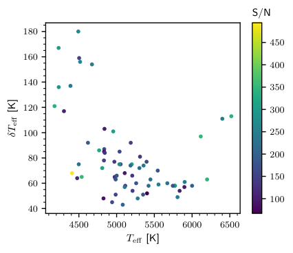
In the cool regime, i.e. K-type stars, where stellar spectra become increasingly more crowded, the continuum placement is more uncertain, and the iron lines are subject to blending with other spectral features. On the other hand, sufficiently strong iron lines become increasingly scarce towards early F-type stars. This has a strong impact on the computed errors in the stellar atmospheric parameters, in particular the effective temperature, and the line-to-line scatter in [Fe/H], as shown in Figs. 8 and 9, respectively.
In Figs. 10 and 11 we compare the stellar atmospheric parameters computed with StePar with values from the literature (McWilliam 1990; Heiter & Luck 2003; Allende Prieto et al. 2004; Valenti & Fischer 2005; Hekker & Meléndez 2007; Liu et al. 2007; Sousa et al. 2008; Takeda et al. 2008; Lyubimkov et al. 2010; Wu et al. 2011; Thygesen et al. 2012; Santos et al. 2013; Morel et al. 2014; Luck 2014; Jofré et al. 2014; Jofré et al. 2015; da Silva et al. 2015; Jofré et al. 2018), taking into account the VIS and NIR channels simultaneously, and only the VIS channel, respectively. To explore possible sources of potential systematic trends or offsets, we followed the Monte Carlo method implemented in Tabernero et al. 2018. We generated 10 000 synthetic samples based on our derived stellar atmospheric parameters. We computed all data points in each of these artificial samples by means of a normal distribution centred at the original measurements, and took the uncertainties in each parameter as the width of the distribution. The summary of the Monte Carlo simulations can be found in Table 2. We computed the Pearson and Spearman correlation coefficients, which quantify the degree of correlation between any two given variables. We found a significant correlation in the differences between our own values and the literature versus the literature values. However, no such correlation was found in the derived and [Fe/H] values.
At first glance, it seems that our temperature scale has an intrinsic systematic error with respect to the literature values. The offset appears to be linked to the fact that we now include the NIR channel, given that the correlation diminishes when we restrict the analysis to the iron lines found in the VIS channel. Although the StePar code could be thought to be the underlying reason for this correlation, we are not comparing the same temperature scale. In other words, we now take into account iron absorption lines in a wavelength region that is different from most studies found in the literature. In addition, this offset is more noticeable for the coolest stars. The former result could arise from the fact that the NIR lines are more sensitive to the effective temperature than the optical lines, at least for the cool stars. In other words, although the inclusion of the NIR in the analysis does not bring extreme differences of the derived stellar parameters with respect to the analysis using the optical range, it seems to reveal a deeper scale as suggested by the meaningful correlation found in Table 2 as well as Figs. 10 and 11.
In Fig. 12 we show the values of derived with StePar against those obtained adopting the distances from Gaia DR2 (Gaia Collaboration et al. 2018), if available, and the Hipparcos mission (van Leeuwen 2007). We computed the latter values by means of the PARAM web interface88 8 http://stev.oapd.inaf.it/cgi-bin/param (da Silva et al. 2006; Rodrigues et al. 2014; Rodrigues et al. 2017), which employs a Bayesian approach to derive the stellar parameters, including stellar age, mass and radius. The values obtained with PARAM can be found in Tables 4 and 5. Following the Monte Carlo method described above, we found a systematic offset of 0.150.38 dex. The Pearson and Spearman correlation coefficients, which are and , respectively, reveal a correlation of around 9%, which is slightly lower than previous works (Tabernero et al. 2017, see e.g.).
Regarding the micro-turbulent velocity, Fig. 13 shows the values of obtained with StePar against the literature. Our derived values for are compatible to the literature values to a large extent. However, six stars (i.e. Dra, F Hya, Mon, Oph, Her, and HD 77912), with computed values larger than 3 km/s, show larger deviations with respect to the literature, which can be as large as 1.6 km s-1. as in the case of the star Mon. In addition, we retrieved a significantly lower value for the star Boo compared to the literature. Although and [Fe/H] are thought to be partially degenerate (Valenti & Fischer 2005), we fail to identify the impact that such high or low values have on [Fe/H] for these stars in our analysis. For example, a difference of 1.6 km s-1 in for the star Mon leads to a difference of only 0.07 dex in [Fe/H] between the literature and the analysis with StePar, and both computed and literature values are compatible within error bars.
A closer look at the comparison between our parameter determinations and the Gaia benchmark star parameters from Heiter et al. 2015, with updated values from Jofré et al. 2018, can be found in Fig. 14. We find good agreement between our derived values and the fundamental and , i.e. derived from the fundamental relations and , respectively, by means of specific information that is available for these stars, such as the parallax, the angular diameter, and the bolometric flux. Nonetheless, we note four outliers in ( K) and two in ( dex). Among the outliers in are Arcturus and 7 Psc. According to Heiter et al. 2015, the value of Arcturus remains uncertain, with literature values ranging from 1.4 up to 2.0 dex, while both the and values for the star 7 Psc are, in fact, not recommended for use as reference values. Among the outliers in are the stars HD 49933, Leo, Vir, and 7 Psc. As stated by Heiter et al. 2015, the fundamental value for the stars Vir and Leo is significantly lower ( 3%) than the value derived in spectroscopic studies. Lastly, at the hot regime, the typical spectroscopic values computed for the star HD 49933 are generally larger.
Lastly, in Fig. 15 we show the final Fe i and Fe ii abundances versus the excitation potential and the reduced equivalent width of the lines, for the four reference CARMENES spectra (18 Sco, Cas, Vir, and Arcturus).
5 Conclusions
In this work, we have expanded previous optical Fe i and Fe ii line lists into the wavelength range covered by CARMENES, i.e. from 5 300 to 17 100 Å. The line lists are suited for FGK-type stars and relate to metal-rich dwarfs (MRD), metal-poor dwarfs (MPD), metal-rich giants (MRG), and metal-poor giants (MPG). For the first time, we provide Fe i and Fe ii lines in the wavelength region between 6 800 Å and 10 000 Å. Altogether, these new line lists contain 653 Fe i and 23 Fe ii lines, of which 351 and 8 are new additions to the line lists compiled in Tabernero et al. 2019, respectively. This implies more than doubling the number of Fe i and Fe ii lines useful for abundance and radial-velocity analyses. The availability of these Fe i and Fe ii line lists is also an asset for other new high-resolution near-infrared spectrographs such as SPIRou, GIANO, CRIRES+, IRD, HPF, and NIRPS that also provide wavelength coverage in the near-infrared wavelength region.
We have reported that the star c Gem (HD 62285) is a new SB2 system, as shown by the cross-correlation with an atlas spectrum of Arcturus.
In addition, we have computed an homogenised set of stellar atmospheric parameters for a sample of 65 FGK-type stars observed with CARMENES by means of the method. We made a comprehensive comparison of our , , and [Fe/H] values with those of virtually all relevant determinations of stellar atmospheric parameters of FGK-type stars. Our parameter determinations are in good agreement with the literature values in general, particularly with the region of the parameter space covered by the YaPSI isochrones (Spada et al. 2017) and the Gaia benchmark stars (Jofré et al. 2014; Jofré et al. 2018; Heiter et al. 2015). The scarcity of Fe ii lines in the NIR wavelength range covered by CARMENES prevented us from performing the stellar parameter determinations using this spectral region alone. However, when using both VIS and NIR CARMENES channel data, we found a broader scale that seems to be linked to a higher sensitivity to effective temperature of the iron lines found in the NIR region.
The line selections provided in this work will be useful for the spectroscopic analysis of any FGK-type star simultaneously observed in the optical and near-infrared wavelength regions. Finally, in a forthcoming publication we plan to expand optical line lists of additional chemical species into the NIR covered by CARMENES and thus assess the impact of the near-infrared wavelength region upon chemical abundance computations for FGK-type stars.
Acknowledgements
CARMENES is an instrument for the Centro Astronómico Hispano en Andalucía at Calar Alto (CAHA). CARMENES is funded by the German Max-Plank Gesellschaft (MPG), the Spanish Consejo Superior de Investigaciones Científicas (CSIC), the European Union through FEDER/ERF FICTS-2011-02 funds, and the members of the CARMENES Consortium (Max-Plank-Institut für Astronomie, Instituto de Astrofísica de Andalucía, Landessternwarte Königstuhl, Institut de Ciències de l’Espai, Institut für Astrophysik Göttingen, Universidad Complutense de Madrid, Thüringer Landessternwarte Tautenberg, Instituto de Astrofísica de Canarias, Hamburger Sternwarte, Centro de Astrobiología and Centro Astronómico Hispano en Andalucía), with additional contributions by the Spanish Ministerio de Economía y Empresa, the German Science Foundation through the Major Research Instrumentation Programme and DFG Research Unit FOR2544 "Blue Planets around Red Stars", the Klaus Tschira Stiftung, the states of Baden-Württemberg and Niedersachsen, and by the Junta de Andalucía. The authors acknowledge financial support from the Fundação para a Ciência e a Tecnologia (FCT) through national funds (PTDC/FIS-AST/28953/2017) and by Fundo Europeu de Desenvolvimento Regional (FEDER) through COMPETE2020 - Programa Operacional Competitividade e Internacionalização (POCI-01-0145-FEDER-028953), and the Spanish Ministerio de Ciencia, Innovación y Universidades, the Universidad Complutense de Madrid, and the Fondo Europeo de Desarrollo Regional (FEDER/ERF) through fellowship FPU15/01476, and projects AYA2016-79425-C3-1/2/3-P. J.I.G.H. acknowledges financial support from the Spanish Ministerio de Ciencia, Innovación y Universidades under the 2013 Ramón y Cajal programme RYC-2013-14875, and from the project AYA2017-86389-P. This work has made use of the VALD database, operated at Uppsala University, the Institute of Astronomy RAS in Moscow, and the University of Vienna. We thank Calar Alto Observatory for the allocation of director’s discretionary time to this programme. E. M. would also like to warmly thank the staff at the Hamburger Sternwarte for their hospitality during his stay funded by project EST18/00162. Based on data from the CARMENES data archive at CAB (INTA-CSIC).
References
- Adibekyan et al. (2014) Adibekyan V. Z., González Hernández J. I., Delgado Mena E., Sousa S. G., Santos N. C., Israelian G., Figueira P., Bertran de Lis S., 2014, A&A, 564, L15
- Allende Prieto et al. (2004) Allende Prieto C., Barklem P. S., Lambert D. L., Cunha K., 2004, A&A, 420, 183
- Allende Prieto et al. (2008) Allende Prieto C., et al., 2008, Astronomische Nachrichten, 329, 1018
- Andreasen et al. (2016) Andreasen D. T., Sousa S. G., Delgado Mena E., Santos N. C., Tsantaki M., Rojas-Ayala B., Neves V., 2016, A&A, 585, A143
- Artigau et al. (2014) Artigau É., et al., 2014, in Ground-based and Airborne Instrumentation for Astronomy V. p. 914715, doi:10.1117/12.2055663
- Aurière (2003) Aurière M., 2003, in Arnaud J., Meunier N., eds, EAS Publications Series Vol. 9, EAS Publications Series. p. 105
- Bensby et al. (2014) Bensby T., Feltzing S., Oey M. S., 2014, A&A, 562, A71
- Blanco-Cuaresma (2019) Blanco-Cuaresma S., 2019, MNRAS, 486, 2075
- Blanco-Cuaresma et al. (2014) Blanco-Cuaresma S., Soubiran C., Heiter U., Jofré P., 2014, iSpec: Stellar atmospheric parameters and chemical abundances, Astrophysics Source Code Library (ascl:1409.006)
- Caballero et al. (2016) Caballero J. A., et al., 2016, in Proc. SPIE. p. 99100E, doi:10.1117/12.2233574
- Clough et al. (2005) Clough S. A., Shephard M. W., Mlawer E. J., Delamere J. S., Iacono M. J., Cady-Pereira K., Boukabara S., Brown P. D., 2005, J. Quant. Spectrosc. Radiative Transfer, 91, 233
- De Medeiros et al. (2000) De Medeiros J. R., do Nascimento J. D. J., Sankarankutty S., Costa J. M., Maia M. R. G., 2000, A&A, 363, 239
- De Medeiros et al. (2002) De Medeiros J. R., Udry S., Burki G., Mayor M., 2002, A&A, 395, 97
- De Silva et al. (2015) De Silva G. M., et al., 2015, MNRAS, 449, 2604
- Delgado Mena et al. (2018) Delgado Mena E., et al., 2018, A&A, 619, A2
- Famaey et al. (2005) Famaey B., Jorissen A., Luri X., Mayor M., Udry S., Dejonghe H., Turon C., 2005, A&A, 430, 165
- Gaia Collaboration et al. (2018) Gaia Collaboration et al., 2018, A&A, 616, A1
- Gilmore et al. (2012) Gilmore G., et al., 2012, The Messenger, 147, 25
- Girard et al. (2000) Girard T. M., et al., 2000, AJ, 119, 2428
- Gontcharov (2006) Gontcharov G. A., 2006, Astronomy Letters, 32, 759
- Gordon et al. (2017) Gordon I. E., Rothman L. S., Tan Y., Kochanov R. V., Hill C., 2017, in 72nd International Symposium on Molecular Spectroscopy. p. TJ08, doi:10.15278/isms.2017.TJ08
- Gray (2018) Gray D. F., 2018, ApJ, 869, 81
- Gray & Toner (1986) Gray D. F., Toner C. G., 1986, ApJ, 310, 277
- Gustafsson et al. (2008) Gustafsson B., Edvardsson B., Eriksson K., Jørgensen U. G., Nordlund Å., Plez B., 2008, A&A, 486, 951
- Hatzes & CRIRES+ Team (2017) Hatzes A., CRIRES+ Team 2017, in American Astronomical Society Meeting Abstracts #230. p. 117.02
- Hayes et al. (2018) Hayes C. R., et al., 2018, ApJ, 852, 49
- Heiter & Luck (2003) Heiter U., Luck R. E., 2003, AJ, 126, 2015
- Heiter et al. (2015) Heiter U., Jofré P., Gustafsson B., Korn A. J., Soubiran C., Thévenin F., 2015, A&A, 582, A49
- Hekker & Meléndez (2007) Hekker S., Meléndez J., 2007, A&A, 475, 1003
- Hinkle et al. (2000) Hinkle K., Wallace L., Valenti J., Harmer D., 2000, Visible and Near Infrared Atlas of the Arcturus Spectrum 3727-9300 A. Astronomical Society of the Pacific
- Jofré et al. (2014) Jofré P., et al., 2014, A&A, 564, A133
- Jofré et al. (2015) Jofré E., Petrucci R., Saffe C., Saker L., de la Villarmois E. A., Chavero C., Gómez M., Mauas P. J. D., 2015, A&A, 574, A50
- Jofré et al. (2018) Jofré P., Heiter U., Tucci Maia M., Soubiran C., Worley C. C., Hawkins K., Blanco-Cuaresma S., Rodrigo C., 2018, Research Notes of the American Astronomical Society, 2, 152
- Jofré et al. (2019) Jofré P., Heiter U., Soubiran C., 2019, ARA&A, 57, 5
- Karataş et al. (2004) Karataş Y., Bilir S., Eker Z., Demircan O., 2004, MNRAS, 349, 1069
- Kasting et al. (1993) Kasting J. F., Whitmire D. P., Reynolds R. T., 1993, Icarus, 101, 108
- Kausch et al. (2015) Kausch W., et al., 2015, A&A, 576, A78
- Keenan & McNeil (1989) Keenan P. C., McNeil R. C., 1989, ApJS, 71, 245
- Kopparapu et al. (2013) Kopparapu R. K., et al., 2013, ApJ, 765, 131
- Kotani et al. (2014) Kotani T., et al., 2014, in Ground-based and Airborne Instrumentation for Astronomy V. p. 914714, doi:10.1117/12.2055075
- Kupka et al. (1999) Kupka F., Piskunov N., Ryabchikova T. A., Stempels H. C., Weiss W. W., 1999, A&AS, 138, 119
- Kupka et al. (2000) Kupka F. G., Ryabchikova T. A., Piskunov N. E., Stempels H. C., Weiss W. W., 2000, Baltic Astronomy, 9, 590
- Lèbre et al. (2006) Lèbre A., de Laverny P., Do Nascimento J. D. J., de Medeiros J. R., 2006, A&A, 450, 1173
- Lebzelter et al. (2012) Lebzelter T., et al., 2012, A&A, 539, A109
- Liu et al. (2007) Liu Y. J., Zhao G., Shi J. R., Pietrzyński G., Gieren W., 2007, MNRAS, 382, 553
- Luck (2014) Luck R. E., 2014, AJ, 147, 137
- Lyubimkov et al. (2010) Lyubimkov L. S., Lambert D. L., Rostopchin S. I., Rachkovskaya T. M., Poklad D. B., 2010, MNRAS, 402, 1369
- Lyubimkov et al. (2012) Lyubimkov L. S., Lambert D. L., Kaminsky B. M., Pavlenko Y. V., Poklad D. B., Rachkovskaya T. M., 2012, MNRAS, 427, 11
- Majewski et al. (2017) Majewski S. R., et al., 2017, AJ, 154, 94
- Maldonado et al. (2010) Maldonado J., Martínez-Arnáiz R. M., Eiroa C., Montes D., Montesinos B., 2010, A&A, 521, A12
- Mann et al. (2019) Mann A. W., et al., 2019, ApJ, 871, 63
- Martínez-Arnáiz et al. (2010) Martínez-Arnáiz R., Maldonado J., Montes D., Eiroa C., Montesinos B., 2010, A&A, 520, A79
- Massarotti et al. (2008) Massarotti A., Latham D. W., Stefanik R. P., Fogel J., 2008, AJ, 135, 209
- Mayor et al. (2003) Mayor M., et al., 2003, The Messenger, 114, 20
- McCarthy & Wilhelm (2014) McCarthy K., Wilhelm R. J., 2014, AJ, 148, 70
- McWilliam (1990) McWilliam A., 1990, ApJS, 74, 1075
- Meléndez & Barbuy (2009) Meléndez J., Barbuy B., 2009, A&A, 497, 611
- Montes et al. (2018) Montes D., et al., 2018, MNRAS, 479, 1332
- Morel et al. (2014) Morel T., et al., 2014, A&A, 564, A119
- Morton (2000) Morton D. C., 2000, ApJS, 130, 403
- Mucciarelli et al. (2013) Mucciarelli A., Pancino E., Lovisi L., Ferraro F. R., Lapenna E., 2013, ApJ, 766, 78
- Nagel et al. (2019) Nagel E., et al., 2019, A&A, submitted
- Nicholls et al. (2017) Nicholls C. P., et al., 2017, A&A, 598, A79
- Nidever et al. (2002) Nidever D. L., Marcy G. W., Butler R. P., Fischer D. A., Vogt S. S., 2002, ApJS, 141, 503
- Oliva et al. (2018) Oliva E., Sanna N., Rainer M., Massi F., Tozzi A., Origlia L., 2018, in Proc. SPIE. p. 1070274, doi:10.1117/12.2309927
- Origlia et al. (2014) Origlia L., et al., 2014, in Proc. SPIE. p. 91471E, doi:10.1117/12.2054743
- Park et al. (2018) Park S., et al., 2018, ApJS, 238, 29
- Passegger et al. (2019) Passegger V. M., et al., 2019, A&A, 627, A161
- Pavlenko et al. (2012) Pavlenko Y. V., Jenkins J. S., Jones H. R. A., Ivanyuk O., Pinfield D. J., 2012, MNRAS, 422, 542
- Piskunov & Valenti (2002) Piskunov N. E., Valenti J. A., 2002, A&A, 385, 1095
- Piskunov & Valenti (2017) Piskunov N., Valenti J. A., 2017, A&A, 597, A16
- Piskunov et al. (1995) Piskunov N. E., Kupka F., Ryabchikova T. A., Weiss W. W., Jeffery C. S., 1995, A&AS, 112, 525
- Pourbaix et al. (2004) Pourbaix D., et al., 2004, A&A, 424, 727
- Press et al. (2002) Press W. H., Teukolsky S. A., Vetterling W. T., Flannery B. P., 2002, Numerical recipes in C++ : the art of scientific computing. Cambridge University Press
- Quirrenbach et al. (2018) Quirrenbach A., et al., 2018, in Ground-based and Airborne Instrumentation for Astronomy VII. p. 107020W, doi:10.1117/12.2313689
- Reiners et al. (2018) Reiners A., et al., 2018, A&A, 612, A49
- Rodrigues et al. (2014) Rodrigues T. S., et al., 2014, MNRAS, 445, 2758
- Rodrigues et al. (2017) Rodrigues T. S., et al., 2017, MNRAS, 467, 1433
- Ryabchikova et al. (2015) Ryabchikova T., Piskunov N., Kurucz R. L., Stempels H. C., Heiter U., Pakhomov Y., Barklem P. S., 2015, Phys. Scr., 90, 054005
- Santos et al. (2013) Santos N. C., et al., 2013, A&A, 556, A150
- Scarfe et al. (1983) Scarfe C. D., Funakawa H., Delaney P. A., Barlow D. J., 1983, J. R. Astron. Soc. Canada, 77, 126
- Schweitzer et al. (2019) Schweitzer A., et al., 2019, A&A, 625, A68
- Skrutskie et al. (2006) Skrutskie M. F., et al., 2006, AJ, 131, 1163
- Smette et al. (2015) Smette A., et al., 2015, A&A, 576, A77
- Sneden (1973) Sneden C. A., 1973, PhD thesis, The University of Texas at Austin
- Soubiran et al. (2013) Soubiran C., Jasniewicz G., Chemin L., Crifo F., Udry S., Hestroffer D., Katz D., 2013, A&A, 552, A64
- Soubiran et al. (2016) Soubiran C., Le Campion J.-F., Brouillet N., Chemin L., 2016, A&A, 591, A118
- Sousa et al. (2007) Sousa S. G., Santos N. C., Israelian G., Mayor M., Monteiro M. J. P. F. G., 2007, A&A, 469, 783
- Sousa et al. (2008) Sousa S. G., et al., 2008, A&A, 487, 373
- Spada et al. (2017) Spada F., Demarque P., Kim Y.-C., Boyajian T. S., Brewer J. M., 2017, ApJ, 838, 161
- Spencer Jones & Furner (1937) Spencer Jones H., Furner H. H., 1937, Monthly Notices of the Royal Astronomical Society, 98, 92
- Steinmetz et al. (2006) Steinmetz M., et al., 2006, AJ, 132, 1645
- Tabernero et al. (2012) Tabernero H. M., Montes D., González Hernández J. I., 2012, A&A, 547, A13
- Tabernero et al. (2017) Tabernero H. M., Montes D., González Hernández J. I., Ammler-von Eiff M., 2017, A&A, 597, A33
- Tabernero et al. (2018) Tabernero H. M., Dorda R., Negueruela I., González-Fernández C., 2018, MNRAS, 476, 3106
- Tabernero et al. (2019) Tabernero H. M., Marfil E., Montes D., González Hernández J. I., 2019, A&A, 628, A131
- Takeda et al. (2005) Takeda Y., et al., 2005, PASJ, 57, 13
- Takeda et al. (2008) Takeda Y., Sato B., Murata D., 2008, PASJ, 60, 781
- Thygesen et al. (2012) Thygesen A. O., et al., 2012, A&A, 543, A160
- Tsantaki et al. (2013) Tsantaki M., Sousa S. G., Adibekyan V. Z., Santos N. C., Mortier A., Israelian G., 2013, A&A, 555, A150
- Valenti & Fischer (2005) Valenti J. A., Fischer D. A., 2005, ApJS, 159, 141
- Wildi et al. (2017) Wildi F., et al., 2017, in Proc. SPIE. p. 1040018, doi:10.1117/12.2275660
- Worek & Beardsley (1977) Worek T. F., Beardsley W. R., 1977, ApJ, 217, 134
- Wright et al. (2018) Wright J. T., et al., 2018, in American Astronomical Society Meeting Abstracts #231. p. 246.45
- Wu et al. (2011) Wu Y., Singh H. P., Prugniel P., Gupta R., Koleva M., 2011, A&A, 525, A71
- Zamora et al. (2015) Zamora O., et al., 2015, AJ, 149, 181
- Zechmeister et al. (2014) Zechmeister M., Anglada-Escudé G., Reiners A., 2014, A&A, 561, A59
- da Silva et al. (2006) da Silva L., et al., 2006, A&A, 458, 609
- da Silva et al. (2015) da Silva R., Milone A. d. C., Rocha-Pinto H. J., 2015, A&A, 580, A24
- dos Santos et al. (2016) dos Santos L. A., et al., 2016, A&A, 592, A156
- van Leeuwen (2007) van Leeuwen F., 2007, A&A, 474, 653
Appendix A Appendix
In Table 3 we give the literature values of the stellar atmospheric parameters for the selected sample. In Tables 4 and 5 we give the stellar atmospheric parameters computed with StePar in the whole VIS+NIR region and VIS region, respectively. In Tables 6 and 7 we list the Fe i and Fe ii lines along with their parameters, respectively, for metal-rich dwarfs (MRD), metal-poor dwarfs (MPD), metal-rich giants (MRG), and metal-poor giants (MPG). Finally, we include the CARMENES spectrum of the reference, metal-rich dwarf 18 Sco in Fig. 16, along with the Fe i and Fe ii lines indicated in red and green, respectively.
| Name | HD | (J2000) | (J2000) | Ref.a | SpTb | Ref.c | Ref.d | [Fe/H] | Ref.e | ||||||
|---|---|---|---|---|---|---|---|---|---|---|---|---|---|---|---|
| [mas] | [km s-1] | [km s-1] | [K] | [dex] | [km s-1] | [dex] | |||||||||
| Metal-rich dwarfs (MRD) | |||||||||||||||
| Sunf | … | … | … | … … | … | G2 V | 0.00 | … | 1.6 | Pav12 | 5771 1 | 4.44 0.00 | 1.20 0.18 | 0.03 0.05 | Jof18 |
| HD 3765 | 3765 | 00 40 49.29 | 40 11 13.3 | 55.7562 0.1002 | G | K2 V | 63.11 | Sou13 | 9.2 | Mar10 | 5032 44 | 4.59 0.06 | 0.85 … | 0.18 0.03 | Val05 |
| HD 100167 | 100167 | 11 31 53.92 | 41 26 21.5 | 28.4793 0.1513 | G | F8 V | 29.49 | Nid02 | 5.0 | McC14 | 5915 44 | 4.38 0.06 | 0.85 … | 0.06 0.03 | Val05 |
| 61 UMa | 101501 | 11 41 03.01 | 34 12 06.4 | 104.3904 0.1287 | G | G8 V | 5.18 | Nid02 | 3.3 | Mar10 | 5488 44 | 4.43 0.06 | 0.85 … | 0.03 0.03 | Val05 |
| Virf | 102870 | 11 50 41.73 | 01 45 52.8 | 89.9258 0.5195 | G | F9 V | 4.71 | Nid02 | 3.4 | Mar10 | 6083 41 | 4.10 0.02 | 1.40 0.09 | 0.24 0.07 | Jof18 |
| CVn | 109358 | 12 33 44.54 | 41 21 27.0 | 116.1298 0.6776 | G | G0 V | 6.52 | Nid02 | 3.2 | Mar10 | 5930 44 | 4.44 0.06 | 0.85 … | 0.16 0.03 | Val05 |
| Com | 114710 | 13 11 52.38 | 27 52 41.1 | 108.8951 0.3487 | G | F9.5 V | 5.46 | Nid02 | 4.7 | Mar10 | 6075 44 | 4.57 0.06 | 0.85 … | 0.07 0.03 | Val05 |
| Boo | 131156 | 14 51 23.28 | 19 06 03.4 | 148.5195 0.2436 | G | G7 Ve+ | 1.59 | Kar04 | 3.3 | Mar10 | 5570 44 | 4.65 0.06 | 0.85 … | 0.04 0.03 | Val05 |
| Ser | 141004 | 15 46 26.61 | 07 21 10.9 | 84.6121 0.2559 | G | G0 IV–V | 66.07 | Nid02 | 3.2 | Mar10 | 5936 44 | 4.30 0.06 | 0.85 … | 0.05 0.03 | Val05 |
| 18 Scof | 146233 | 16 15 37.26 | 08 22 09.6 | 70.7675 0.1119 | G | G2 Va | 11.90 | Gaia | 2.1 | San16 | 5810 80 | 4.44 0.03 | 1.20 0.20 | 0.03 0.03 | Jof18 |
| HD 166620 | 166620 | 18 09 37 45 | 38 27 28.8 | 90.1264 0.0200 | G | K2 V | 19.47 | Sou13 | 4.8 | Mar10 | 5000 44 | 4.47 0.06 | 0.85 … | 0.18 0.03 | Val05 |
| HD 182488 | 182488 | 19 23 34.01 | 33 13 19.1 | 64.0623 0.0218 | G | G9 V | 21.47 | Sou13 | 0.6 | Fek97 | 5453 44 | 4.67 0.06 | 0.85 … | 0.22 0.03 | Val05 |
| Dra | 185144 | 19 32 21.53 | 69 39 41.3 | 173.2405 0.2070 | G | G9 V | 26.78 | Nid02 | 6.8 | Mar10 | 5218 96 | 4.61 0.05 | 1.07 … | 0.25 0.02 | All04 |
| HD 219134 | 219134 | 23 13 16.92 | 57 10 05.9 | 153.0808 0.0895 | G | K3 V | 18.83 | Nid02 | 6.9 | Mar10 | 4743 86 | 4.63 0.04 | 1.00 … | 0.12 0.02 | All04 |
| Metal-poor dwarfs (MPD) | |||||||||||||||
| Cas | 4614 | 00 49 06.22 | 57 48 54.5 | 171.2861 0.5815 | G | F9 V+ | 8.44 | Nid02 | 3.2 | Mar10 | 5900 50 | 4.50 0.05 | 0.90 0.05 | 0.35 0.04 | Hei03 |
| Casf | 6582 | 01 08 15.97 | 54 55 14.8 | 132.38 0.82 | H | K1 V | 98.10 | Pou04 | 4.2 | Mar10 | 5308 29 | 4.41 0.06 | 1.10 0.29 | 0.81 0.03 | Jof18 |
| HD 49933f | 49933 | 06 50 49.83 | 00 32 27.0 | 33.4441 0.0891 | G | F3 V | 12.65 | Gaia | 5.0 | Tak05 | 6635 91 | 4.20 0.03 | 1.90 0.35 | 0.41 0.08 | Jof18 |
| CF UMaf | 103095 | 11 52 58.80 | 37 43 06.0 | 108.9551 0.0490 | G | G8 Vp | 97.49 | Hay18 | 9.3 | Mar10 | 5140 55 | 4.60 0.03 | 1.10 0.57 | 1.46 0.39 | Jof18 |
| HD 154363 | 154363 | 17 03 07.86 | 14 05 31.0 | 95.5499 0.0651 | G | K4 V | 34.22 | Mon18 | 1.9 | Mar10 | 4723 89 | 4.41 0.24 | … … | 0.62 0.04 | Sou08 |
| Metal-rich giants (MRG) | |||||||||||||||
| Gem | 58207 | 07 25 43.59 | 27 47 52.9 | 24.8793 0.3562 | G | G9 IIIb | 7.26 | Mas08 | 0.0 | Mas08 | 4912 56 | 2.82 0.28 | 1.47 0.09 | 0.03 0.10 | Sil15 |
| CMif | 61421 | 07 39 18.05 | 05 13 29.8 | 284.56 1.26 | H | F5 IV–V | 4.10 | Mal10 | 5.4 | Mar10 | 6554 84 | 4.00 0.02 | 1.80 0.11 | 0.01 0.08 | Jof18 |
| Gem | 62345 | 07 44 26.84 | 24 23 52.6 | 23.6199 0.3954 | G | G8 IIIa | 20.15 | Sou08 | 3.3 | Mas08 | 5120 28 | 2.98 0.16 | 1.56 0.04 | 0.03 0.05 | Sil15 |
| Gemf | 62509 | 07 45 18.91 | 28 01 34.0 | 96.54 0.27 | H | K0 IIIb | 3.23 | Jof15 | 2.3 | Jof15 | 4858 60 | 2.90 0.08 | 1.10 0.21 | 0.13 0.16 | Jof18 |
| Mon | 67594 | 08 08 35.65 | 02 59 01.5 | 4.7723 0.3259 | G | G2 Iab/b | 31.20 | Gaia | 6.7 | Med02 | 5210 100 | 1.75 0.07 | 3.3 0.5 | 0.01 0.12 | Lyu10 |
| Cnc | 69267 | 08 16 30.90 | 09 11 08.0 | 11.0443 0.6561 | G | K4 III | 22.94 | Fam05 | 6.9 | Mas08 | 4200 … | 2.05 … | 2.30 … | 0.19 … | Hek07 |
| F Hya | 74395 | 08 43 40.37 | 07 14 01.2 | 1.8273 0.2985 | G | G0/2 Ib | 27.68 | Gaia | 7.5 | Med02 | 5370 100 | 2.08 0.06 | 3.5 0.5 | 0.03 0.13 | Lyu10 |
| Hya | 76294 | 08 55 23.62 | 05 56 44.1 | 20.7182 0.3925 | G | G9 II–III | 22.30 | Gon06 | 2.5 | Mas08 | 5049 55 | 2.88 0.30 | 1.67 0.08 | 0.01 0.11 | Sil15 |
| HD 77912 | 77912 | 09 06 31.77 | 38 27 08.0 | 5.0045 0.1977 | G | G7 II | 16.04 | Gaia | 1.5 | Med02 | 5001 … | 2.03 … | 2.16 … | 0.12 … | Luc14 |
| Hya | 81797 | 09 27 35.24 | 08 39 30.8 | 18.09 0.18 | H | K3 IIIa | 4.27 | Jof15 | 4.0 | Jof15 | 4395 37 | 2.09 0.11 | 1.76 0.12 | 0.11 0.05 | Jof15 |
| DK UMa | 82210 | 09 34 28.88 | 69 49 49.0 | 30.9269 0.1621 | G | G5 III–IV | 27.07 | Gaia | 5.5 | Med00 | 5343 33 | 3.49 0.08 | … … | 0.21 0.07 | Wu11 |
| 10 LMi | 82635 | 09 34 13.38 | 36 23 51.3 | 18.1458 0.2345 | G | G8.5 III | 11.94 | Mas08 | 6.5 | Mas08 | 5195 40 | 3.26 0.26 | 1.56 0.06 | 0.02 0.07 | Sil15 |
| Leo | 84441 | 09 45 51.08 | 23 46 27.3 | 11.1759 0.9166 | G | G1 II | 4.48 | Sou08 | 8.1 | Mas08 | 5383 … | 2.17 … | 2.09 … | 0.04 … | Luc14 |
| Leof | 85503 | 09 52 45.85 | 26 00 24.8 | 30.6493 0.4219 | G | K2 III | 13.63 | Fam05 | 4.5 | Mas08 | 4474 60 | 2.51 0.11 | … … | 0.25 0.15 | Jof18 |
| LMi | 90537 | 10 27 53.02 | 36 42 25.9 | 21.19 0.50 | H | G9 IIIb | 8.52 | Gaia | 7.1 | Mas08 | 5060 … | 2.95 … | 2.1 … | 0.00 0.10 | McW90 |
| 37 LMi | 92125 | 10 38 43.21 | 31 58 34.6 | 5.2136 0.4108 | G | G3 Ib–II | 7.71 | Gaia | 9.5 | Lyu12 | 5475 50 | 2.36 0.04 | 2.7 0.5 | 0.02 0.11 | Lyu10 |
| UMa | 95689 | 11 03 43.64 | 61 45 03.4 | 26.54 0.48 | H | G8 III+ | 9.40 | Gon06 | 2.7 | Gra18 | 4660 … | 2.46 … | 2.2 … | 0.20 0.07 | McW90 |
| UMa | 96833 | 11 09 39.79 | 44 29 54.4 | 21.0443 0.5249 | G | K1 III | 3.39 | Fam05 | 5.5 | Mas08 | 4600 22 | 1.95 0.08 | … … | 0.03 0.08 | Thy12 |
| UMa | 98262 | 11 18 28.74 | 33 05 39.3 | 14.2521 0.5672 | G | K3 III | 9.63 | Fam05 | 2.7 | Med00 | 4120 … | 1.86 … | 2.4 … | 0.20 0.12 | McW90 |
| 56 UMa | 98839 | 11 22 49.58 | 43 28 57.7 | 5.8742 0.1937 | G | G8 IIIa | 1.01 | Pou04 | 4.0 | Leb06 | 4936 25 | 2.30 0.08 | 1.78 0.10 | 0.05 0.04 | Tak08 |
| Virf | 113226 | 13 02 10.59 | 10 57 32.9 | 30.5624 0.4379 | G | G8 III | 14.29 | Jof15 | 1.4 | Jof15 | 4983 61 | 2.77 0.02 | 1.10 0.25 | 0.15 0.16 | Jof18 |
| Boof | 121370 | 13 54 41.06 | 18 23 51.4 | 87.75 1.24 | H | G0 IV | 0.70 | Jof15 | 12.3 | Jof15 | 6099 28 | 3.79 0.02 | 1.92 0.03 | 0.32 0.08 | Jof15 |
| Boo | 127665 | 14 31 49.77 | 30 22 16.9 | 21.9348 0.3952 | G | K3 III | 13.57 | Mas08 | 5.0 | Mas08 | 4258 65 | 1.85 0.36 | 1.59 0.12 | 0.13 0.12 | Sil15 |
| UMi | 131873 | 14 50 42.35 | 74 09 19.9 | 24.91 0.12 | H | K4 III | 16.96 | Fam05 | 1.6 | Gon99 | 4067 13 | 1.70 0.11 | … … | 0.13 0.05 | Wu11 |
| Boo | 135722 | 15 15 30.15 | 33 18 53.7 | 26.7797 0.3806 | G | G8 IV | 12.29 | Sou08 | 3.6 | Mas08 | 4982 28 | 2.89 0.19 | 1.44 0.04 | 0.23 0.06 | Sil15 |
| Dra | 137759 | 15 24 55.78 | 58 57 57.7 | 31.5727 0.2959 | G | K2 III | 12.31 | Gaia | 1.9 | Jof15 | 4504 16 | 2.52 0.07 | 1.41 0.07 | 0.03 0.04 | Jof15 |
| Ser | 140573 | 15 44 16.05 | 06 25 32.4 | 39.3696 0.8514 | G | K2 IIIb | 2.63 | Fam05 | 4.3 | Mas08 | 4496 … | 2.52 … | 1.5 0.2 | 0.17 … | Liu07 |
| CrB | 142091 | 15 51 13.94 | 35 39 26.4 | 33.2328 0.1083 | G | K0 III–IV | 23.16 | Jof15 | 1.4 | Jof15 | 4803 25 | 3.23 0.04 | 0.83 0.06 | 0.17 0.05 | Jof15 |
| CrB | 143107 | 15 57 35.23 | 26 52 40.0 | 14.2898 0.2149 | G | K2 III | 32.42 | Fam05 | 2.4 | Mas08 | 4436 56 | 1.94 0.15 | 1.68 0.06 | 0.22 0.03 | San13 |
| Oph | 146791 | 16 18 19.28 | 04 41 32.7 | 30.2620 0.7915 | G | G9.5 IIIb | 9.18 | Mas08 | 3.6 | Mas08 | 4940 55 | 2.64 0.06 | 1.43 0.06 | 0.04 0.10 | Mor14 |
| Her | 150680 | 16 41 17.28 | 31 36 09.3 | 93.32 0.47 | H | G1 IV | 67.80 | Gon06 | 3.1 | Mar10 | 5655 148 | 3.67 0.12 | 1.38 … | 0.01 0.02 | All04 |
| Oph | 153210 | 16 57 40.07 | 09 22 29.9 | 36.8142 0.4578 | G | K2 III | 55.85 | Mas08 | 4.7 | Mas08 | 4655 … | 2.70 … | 1.82 … | 0.07 … | Hek07 |
| Her | 156283 | 17 15 02.85 | 36 48 32.9 | 9.1810 0.4201 | G | K3 II | 25.57 | Fam05 | 1.3 | Leb06 | 4170 … | 1.90 … | 2.26 … | 0.01 … | Hek07 |
| Oph | 157999 | 17 26 30.87 | 04 08 25.2 | 3.8431 0.2836 | G | K2 III | 27.81 | Fam05 | 4.2 | Leb06 | 4080 … | 1.52 … | 2.54 … | 0.07 … | Hek07 |
| Dra | 159181 | 17 30 25.97 | 52 18 05.1 | 8.1882 0.5562 | G | G2 Ib–IIa | 21.00 | Sou08 | 10.7 | Leb06 | 5160 150 | 1.86 0.04 | 3.0 0.5 | 0.02 0.10 | Lyu10 |
| Oph | 161096 | 17 43 28.35 | 04 34 02.2 | 40.0945 0.6752 | G | K2 III | 12.53 | Fam05 | 5.4 | Mas08 | 4680 … | 2.95 … | 2.02 … | 0.13 … | Hek07 |
| Her | 161797 | 17 46 27.52 | 27 43 14.2 | 119.1128 0.4848 | G | G5 IV | 17.69 | Mon18 | 1.7 | Jof15 | 5562 35 | 3.98 0.05 | 1.02 0.07 | 0.28 0.05 | Jof15 |
| Dra | 163588 | 17 53 31.73 | 56 52 21.6 | 29.8654 0.3051 | G | K2 III | 26.46 | Mas08 | 2.3 | Mas08 | 4702 76 | 2.94 0.33 | 1.41 0.21 | 0.12 0.14 | Sil15 |
| Her | 163770 | 17 56 15.17 | 37 15 01.9 | 2.7547 0.2684 | G | K1 II+ | 28.32 | Fam05 | 3.4 | Gra86 | 4255 … | 1.25 … | 2.75 … | 0.11 … | Hek07 |
| Her | 163993 | 17 57 45.88 | 29 14 52.3 | 25.2599 0.3303 | G | G8 III | 1.72 | Fam05 | 2.8 | Mas08 | 5220 51 | 3.28 0.26 | 1.62 0.08 | 0.06 0.09 | Sil15 |
| Oph | 163917 | 17 59 01.60 | 09 46 24.9 | 23.0524 0.4626 | G | K1 III | 13.19 | Jof15 | 2.8 | Jof15 | 4997 56 | 2.84 0.09 | 1.60 0.05 | 0.05 0.07 | Jof15 |
| Metal-poor giants (MPG) | |||||||||||||||
| c Virf | 107328 | 12 20 20.99 | 03 18 45.3 | 9.7577 0.2536 | G | K0 IIIb | 36.66 | Gaia | 1.9 | Mas08 | 4496 59 | 2.09 0.13 | 1.20 0.26 | 0.33 0.16 | Jof18 |
| Boo | 120477 | 13 49 28.67 | 15 47 52.3 | 14.2758 0.3494 | G | K5.5 III | 5.85 | Fam05 | 5.1 | Mas08 | 4170 … | 1.60 … | 2.60 … | 0.57 … | Hek07 |
| Arcturusf | 124897 | 14 15 39.68 | 19 10 55.8 | 88.83 0.54 | H | K1.5 III | 5.19 | Mas08 | 4.2 | Mas08 | 4286 35 | 1.60 0.20 | 1.30 0.12 | 0.52 0.08 | Jof18 |
| Lib | 138905 | 15 35 31.57 | 14 47 22.2 | 21.0823 0.4010 | G | G8.5 III | 26.71 | Jof15 | 1.6 | Jof15 | 4786 13 | 2.55 0.04 | 1.36 0.05 | 0.30 0.03 | Jof15 |
| 7 Pscf | 220009 | 23 20 20.58 | 05 22 52.8 | 9.5042 0.1880 | G | K1 IV | 40.46 | Gaia | 1.0 | Med00 | 4266 60 | 1.43 0.12 | 1.30 0.14 | 0.74 0.13 | Jof14 |
| a References for parallax, : G:Gaia DR2 (Gaia Collaboration et al. 2018); H: Hipparcos (van Leeuwen 2007). | |||||||||||||||
| b Reference for spectral type, SpT: Caballero et al. (in prep.). | |||||||||||||||
| c References for : Fam05: Famaey et al. 2005; Gaia: Gaia Collaboration et al. 2018; Gon06: Gontcharov 2006; Hay18: Hayes et al. 2018; Kar04: Karataş et al. 2004; Jof15: Jofré et al. 2015; Mal10: Maldonado et al. 2010; Mas08: Massarotti et al. 2008; Mon18: Montes et al. 2018; Nid02: Nidever et al. 2002; Pou04: Pourbaix et al. 2004; Sou13: Soubiran et al. 2013. | |||||||||||||||
| d References for : San16: dos Santos et al. 2016; Jof15: Jofré et al. 2015; Gra86: Gray & Toner 1986; Gra18: Gray 2018; Leb06: Lèbre et al. 2006; Lyu12: Lyubimkov et al. 2012; Mar10: Martínez-Arnáiz et al. 2010; Mas08: Massarotti et al. 2008; McC14: McCarthy & Wilhelm 2014; Med00: De Medeiros et al. 2000; Med02: De Medeiros et al. 2002; Pav12: Pavlenko et al. 2012; Tak05: Takeda et al. 2005. | |||||||||||||||
| e References for , , , and [Fe/H]: All04: Allende Prieto et al. 2004; Hei03: Heiter & Luck 2003; Hek07: Hekker & Meléndez 2007; Jof14: Jofré et al. 2014; Jof15: Jofré et al. 2015; Jof18: Jofré et al. 2018; Liu07: Liu et al. 2007; Luc14: Luck 2014; Lyu10: Lyubimkov et al. 2010; McW90: McWilliam 1990; Mor14: Morel et al. 2014; San13: Santos et al. 2013; Sil15: da Silva et al. 2015; Sou08: Sousa et al. 2008; Tak08: Takeda et al. 2008; Thy12: Thygesen et al. 2012; Val05: Valenti & Fischer 2005; Wu11: Wu et al. 2011. | |||||||||||||||
| f Gaia benchmark star (Jofré et al. 2014; Jofré et al. 2018; Heiter et al. 2015). | |||||||||||||||
| Name | S/N | [Fe/H] | |||||
|---|---|---|---|---|---|---|---|
| [km s-1] | [K] | [dex] | [dex] | [km s-1] | [dex] | ||
| Metal-rich dwarfs (MRD) | |||||||
| Sun | 0.00 0.00 | 249 | 5768 58 | 4.45 0.12 | … … | 1.31 0.09 | 0.01 0.04 |
| HD 3765 | 63.18 0.50 | 138 | 5310 81 | 4.63 0.24 | 4.55 0.02 | 1.43 0.10 | 0.12 0.03 |
| HD 100167 | 29.41 0.52 | 98 | 5898 57 | 4.47 0.12 | 4.43 0.02 | 1.27 0.09 | 0.01 0.04 |
| 61 UMa | 5.47 0.46 | 248 | 5555 59 | 4.59 0.13 | 4.52 0.02 | 1.36 0.10 | 0.07 0.03 |
| Vir | 4.58 0.65 | 345 | 6199 63 | 4.23 0.13 | 4.09 0.02 | 1.53 0.08 | 0.17 0.04 |
| CVn | 6.34 0.49 | 241 | 5902 61 | 4.41 0.13 | 4.37 0.03 | 1.22 0.10 | 0.20 0.04 |
| Com | 5.41 0.57 | 198 | 6000 58 | 4.44 0.12 | 4.42 0.01 | 1.30 0.08 | 0.04 0.04 |
| Boo | 1.81 0.40 | 67 | 5403 52 | 4.48 0.12 | 4.54 0.02 | 1.45 0.08 | 0.19 0.03 |
| Ser | 66.22 0.60 | 109 | 5835 54 | 4.00 0.14 | 4.22 0.02 | 1.34 0.07 | 0.04 0.04 |
| 18 Sco | 11.93 0.59 | 298 | 5774 58 | 4.43 0.13 | 4.41 0.04 | 1.30 0.08 | 0.00 0.04 |
| HD 166620 | 19.26 0.44 | 163 | 5039 85 | 4.66 0.21 | 4.56 0.02 | 0.88 0.13 | 0.19 0.03 |
| HD 182488 | 21.39 0.45 | 178 | 5545 70 | 4.59 0.16 | 4.51 0.02 | 1.34 0.10 | 0.17 0.04 |
| Dra | 26.77 0.55 | 183 | 5259 60 | 4.52 0.14 | 4.56 0.02 | 0.97 0.09 | 0.23 0.03 |
| HD 219134 | 18.54 0.57 | 149 | 5187 92 | 4.71 0.28 | 4.57 0.02 | 1.28 0.12 | 0.04 0.03 |
| Metal-poor dwarfs (MPD) | |||||||
| Cas | 8.41 0.92 | 246 | 5807 49 | 4.39 0.12 | 4.33 0.02 | 1.07 0.07 | 0.32 0.04 |
| Cas | 96.99 0.81 | 245 | 5279 48 | 4.35 0.13 | 4.39 0.03 | 1.09 0.08 | 0.90 0.03 |
| HD 49933 | 12.14 1.72 | 248 | 6401 111 | 4.16 0.19 | 4.17 0.04 | 1.27 0.09 | 0.59 0.07 |
| CF UMa | 97.88 0.91 | 201 | 5081 43 | 4.40 0.30 | 4.69 0.02 | 1.31 0.09 | 1.41 0.03 |
| HD 154363 | 34.27 0.78 | 96 | 5107 68 | 4.35 0.24 | 4.73 0.01 | 1.07 0.14 | 0.71 0.05 |
| Metal-rich giants (MRG) | |||||||
| Gem | 7.08 0.20 | 268 | 4981 64 | 2.76 0.22 | 2.72 0.08 | 1.71 0.08 | 0.01 0.04 |
| CMi | 4.98 0.89 | 341 | 6520 113 | 3.77 0.18 | 3.98 0.03 | 1.50 0.10 | 0.02 0.06 |
| Gem | 19.84 0.11 | 318 | 5201 75 | 3.00 0.25 | 2.83 0.02 | 1.93 0.12 | 0.07 0.05 |
| Gem | 3.12 0.12 | 130 | 4974 65 | 2.91 0.24 | 2.83 0.04 | 1.46 0.07 | 0.11 0.04 |
| Mon | 29.32 0.33 | 239 | 5357 74 | 1.94 0.25 | 1.95 0.06 | 4.87 0.85 | 0.06 0.06 |
| Cnc | 22.24 0.11 | 270 | 4492 180 | 1.84 0.71 | 1.43 0.16 | 2.30 0.17 | 0.21 0.14 |
| F Hya | 26.86 0.25 | 169 | 5397 77 | 1.92 0.19 | 1.71 0.06 | 3.57 0.39 | 0.04 0.06 |
| Hya | 22.71 0.13 | 182 | 4987 63 | 2.61 0.22 | 2.50 0.02 | 1.80 0.10 | 0.02 0.05 |
| HD 77912 | 15.94 0.11 | 153 | 5053 75 | 2.24 0.30 | 1.94 0.06 | 3.63 0.40 | 0.09 0.05 |
| Hya | 4.48 0.11 | 267 | 4516 156 | 1.69 0.62 | 1.67 0.05 | 2.15 0.14 | 0.08 0.12 |
| DK UMa | 26.99 0.62 | 180 | 5351 51 | 3.54 0.14 | 3.37 0.02 | 1.35 0.07 | 0.15 0.04 |
| 10 LMi | 11.95 0.11 | 134 | 5207 66 | 3.05 0.22 | 3.00 0.02 | 1.81 0.10 | 0.00 0.05 |
| Leo | 4.45 0.17 | 219 | 5448 63 | 2.34 0.19 | 2.27 0.07 | 2.31 0.15 | 0.05 0.05 |
| Leo | 13.75 0.08 | 100 | 4839 103 | 2.64 0.42 | 2.52 0.08 | 1.85 0.12 | 0.25 0.07 |
| LMi | 8.11 0.10 | 217 | 5184 74 | 3.06 0.24 | 2.80 0.05 | 1.54 0.09 | 0.16 0.05 |
| 37 LMi | 8.58 0.14 | 221 | 5423 58 | 2.04 0.18 | 2.31 0.06 | 2.45 0.15 | 0.02 0.04 |
| UMa | 11.97 0.45 | 312 | 4809 72 | 2.22 0.30 | 2.04 0.11 | 1.99 0.11 | 0.06 0.05 |
| UMa | 4.26 0.09 | 324 | 4768 86 | 2.34 0.34 | 2.21 0.13 | 1.77 0.10 | 0.01 0.06 |
| UMa | 9.18 0.08 | 293 | 4233 136 | 1.73 0.55 | 1.44 0.14 | 2.04 0.11 | 0.17 0.10 |
| 56 UMa | 0.44 0.34 | 276 | 5037 75 | 2.59 0.26 | 2.23 0.03 | 2.47 0.17 | 0.00 0.05 |
| Vir | 14.09 0.08 | 145 | 5211 54 | 2.90 0.21 | 2.64 0.03 | 1.72 0.08 | 0.16 0.04 |
| Boo | 1.64 0.52 | 348 | 6115 97 | 3.86 0.20 | 3.79 0.02 | 1.95 0.12 | 0.28 0.06 |
| Boo | 13.86 0.07 | 190 | 4620 92 | 2.31 0.36 | 1.91 0.08 | 1.96 0.09 | 0.07 0.07 |
| UMi | 16.58 0.21 | 304 | 4231 167 | 2.06 0.59 | 1.39 0.04 | 2.13 0.15 | 0.16 0.12 |
| Boo | 12.05 0.55 | 162 | 4940 45 | 2.58 0.17 | 2.67 0.05 | 1.50 0.06 | 0.29 0.03 |
| Dra | 10.96 0.22 | 175 | 4836 87 | 2.86 0.33 | 2.35 0.07 | 1.79 0.09 | 0.13 0.06 |
| Ser | 2.63 0.09 | 84 | 4834 85 | 2.75 0.34 | 2.34 0.13 | 1.75 0.09 | 0.23 0.06 |
| CrB | 25.02 0.26 | 142 | 4970 77 | 3.29 0.27 | 3.17 0.03 | 1.44 0.08 | 0.09 0.04 |
| CrB | 31.88 0.11 | 224 | 4498 75 | 2.46 0.26 | 1.92 0.08 | 1.57 0.06 | 0.03 0.06 |
| Oph | 9.43 0.17 | 155 | 4987 51 | 2.74 0.18 | 2.66 0.11 | 1.60 0.07 | 0.05 0.04 |
| Her | 70.12 0.53 | 173 | 5745 58 | 3.72 0.14 | 3.70 0.06 | 1.52 0.08 | 0.03 0.04 |
| Oph | 55.39 0.12 | 155 | 4832 78 | 2.56 0.29 | 2.46 0.14 | 1.77 0.08 | 0.14 0.05 |
| Her | 25.45 0.11 | 109 | 4302 117 | 1.74 0.51 | 1.42 0.11 | 2.42 0.18 | 0.07 0.09 |
| Oph | 26.83 0.12 | 157 | 4503 159 | 2.02 0.54 | 1.14 0.11 | 3.57 0.42 | 0.12 0.10 |
| Dra | 20.44 0.21 | 217 | 5302 72 | 1.79 0.22 | 1.78 0.06 | 3.43 0.35 | 0.06 0.06 |
| Oph | 12.23 0.11 | 301 | 4955 101 | 3.15 0.35 | 2.54 0.10 | 2.08 0.15 | 0.28 0.06 |
| Her | 18.03 0.39 | 233 | 5672 60 | 4.08 0.17 | 3.99 0.02 | 1.36 0.07 | 0.30 0.04 |
| Dra | 26.12 0.07 | 136 | 4843 84 | 2.69 0.39 | 2.73 0.11 | 1.79 0.10 | 0.06 0.06 |
| Her | 28.60 0.12 | 237 | 4388 137 | 1.84 0.52 | 0.97 0.12 | 3.86 0.42 | 0.02 0.08 |
| Her | 1.72 0.15 | 237 | 5107 57 | 2.74 0.23 | 2.96 0.03 | 1.61 0.07 | 0.09 0.04 |
| Oph | 12.35 0.11 | 176 | 5001 66 | 2.61 0.22 | 2.63 0.03 | 1.73 0.07 | 0.15 0.04 |
| Metal-poor giants (MPG) | |||||||
| c Vir | 36.55 0.13 | 353 | 4537 65 | 2.23 0.28 | 1.96 0.11 | 1.64 0.06 | 0.29 0.05 |
| Boo | 5.84 0.10 | 342 | 4177 121 | 1.94 0.48 | 1.67 0.09 | 1.40 0.09 | 0.60 0.15 |
| Boo | 4.71 0.11 | 494 | 4409 68 | 2.06 0.26 | 1.64 0.05 | 1.52 0.05 | 0.37 0.06 |
| Lib | 26.07 0.14 | 88 | 4826 48 | 2.81 0.18 | 2.37 0.06 | 1.42 0.05 | 0.26 0.03 |
| 7 Psc | 40.51 0.09 | 117 | 4477 64 | 2.14 0.25 | 1.75 0.05 | 1.44 0.05 | 0.59 0.05 |
| Name | S/N | [Fe/H] | |||||
|---|---|---|---|---|---|---|---|
| [km s-1] | [K] | [dex] | [dex] | [km s-1] | [dex] | ||
| Metal-rich dwarfs (MRD) | |||||||
| Sun | 0.00 0.00 | 249 | 5787 54 | 4.42 0.11 | … … | 0.98 0.08 | 0.02 0.03 |
| HD 3765 | 63.18 0.50 | 138 | 5206 84 | 4.62 0.22 | 4.55 0.02 | 1.17 0.12 | 0.16 0.04 |
| HD 100167 | 29.41 0.52 | 98 | 5942 54 | 4.49 0.10 | 4.43 0.02 | 1.04 0.09 | 0.04 0.04 |
| 61 UMa | 5.47 0.46 | 248 | 5576 56 | 4.56 0.12 | 4.52 0.02 | 1.07 0.09 | 0.01 0.03 |
| Vir | 4.58 0.65 | 345 | 6255 64 | 4.20 0.12 | 4.09 0.02 | 1.45 0.08 | 0.23 0.04 |
| CVn | 6.34 0.49 | 241 | 5967 57 | 4.40 0.12 | 4.37 0.03 | 0.96 0.09 | 0.14 0.04 |
| Com | 5.41 0.57 | 198 | 6105 56 | 4.42 0.11 | 4.42 0.01 | 1.18 0.07 | 0.02 0.04 |
| Boo | 1.81 0.40 | 67 | 5536 55 | 4.50 0.12 | 4.54 0.02 | 1.25 0.09 | 0.15 0.03 |
| Ser | 66.22 0.60 | 109 | 5950 56 | 4.31 0.14 | 4.22 0.02 | 1.22 0.08 | 0.05 0.04 |
| 18 Sco | 11.93 0.59 | 298 | 5786 54 | 4.40 0.10 | 4.41 0.04 | 0.99 0.09 | 0.02 0.04 |
| HD 166620 | 19.26 0.44 | 163 | 5048 64 | 4.63 0.15 | 4.56 0.02 | 0.80 0.18 | 0.14 0.02 |
| HD 182488 | 21.39 0.45 | 178 | 5543 67 | 4.66 0.17 | 4.51 0.02 | 1.12 0.10 | 0.24 0.04 |
| Dra | 26.77 0.55 | 183 | 5278 60 | 4.50 0.13 | 4.56 0.02 | 0.79 0.11 | 0.20 0.05 |
| HD 219134 | 18.54 0.57 | 149 | 5162 84 | 4.72 0.25 | 4.57 0.02 | 1.08 0.13 | 0.10 0.05 |
| Metal-poor dwarfs (MPD) | |||||||
| Cas | 8.41 0.92 | 246 | 5861 53 | 4.45 0.12 | 4.33 0.02 | 0.89 0.09 | 0.27 0.04 |
| Cas | 96.99 0.81 | 245 | 5350 56 | 4.49 0.15 | 4.39 0.03 | 0.87 0.22 | 0.77 0.04 |
| HD 49933 | 12.14 1.72 | 248 | 6665 102 | 4.18 0.17 | 4.17 0.04 | 1.32 0.09 | 0.41 0.06 |
| CF UMa | 97.88 0.91 | 201 | 5101 51 | 4.38 0.32 | 4.69 0.02 | 1.27 0.10 | 1.38 0.04 |
| HD 154363 | 34.27 0.78 | 96 | 5082 86 | 4.32 0.56 | 4.73 0.01 | 1.12 0.13 | 0.60 0.06 |
| Metal-rich giants (MRG) | |||||||
| Gem | 7.08 0.20 | 268 | 4905 70 | 2.55 0.26 | 2.72 0.08 | 1.57 0.08 | 0.02 0.05 |
| CMi | 4.98 0.89 | 341 | 6593 92 | 4.01 0.11 | 3.98 0.03 | 1.52 0.08 | 0.03 0.05 |
| Gem | 19.84 0.11 | 318 | 5194 88 | 3.06 0.26 | 2.83 0.02 | 1.74 0.12 | 0.11 0.06 |
| Gem | 3.12 0.12 | 130 | 4930 79 | 2.78 0.31 | 2.83 0.04 | 1.36 0.09 | 0.12 0.06 |
| Mon | 29.32 0.33 | 239 | 5346 77 | 1.74 0.23 | 1.95 0.06 | 4.56 0.26 | 0.06 0.06 |
| Cnc | 22.24 0.11 | 270 | 4357 126 | 1.79 0.52 | 1.43 0.16 | 1.98 0.14 | 0.16 0.13 |
| F Hya | 26.86 0.25 | 169 | 5331 75 | 1.84 0.20 | 1.71 0.06 | 2.71 0.20 | 0.01 0.06 |
| Hya | 22.71 0.13 | 182 | 4980 74 | 2.68 0.27 | 2.50 0.02 | 1.66 0.09 | 0.04 0.06 |
| HD 77912 | 15.94 0.11 | 153 | 5006 83 | 2.19 0.28 | 1.94 0.06 | 2.55 0.19 | 0.00 0.06 |
| Hya | 4.48 0.11 | 267 | 4450 115 | 1.45 0.49 | 1.67 0.05 | 2.00 0.12 | 0.11 0.10 |
| DK UMa | 26.99 0.62 | 180 | 5379 51 | 3.65 0.15 | 3.37 0.02 | 1.24 0.07 | 0.17 0.04 |
| 10 LMi | 11.95 0.11 | 134 | 5195 74 | 3.12 0.23 | 3.00 0.02 | 1.52 0.10 | 0.08 0.06 |
| Leo | 4.45 0.17 | 219 | 5472 72 | 2.45 0.18 | 2.27 0.07 | 2.12 0.13 | 0.02 0.06 |
| Leo | 13.75 0.08 | 100 | 4789 127 | 2.63 0.46 | 2.52 0.08 | 1.56 0.12 | 0.30 0.09 |
| LMi | 8.11 0.10 | 217 | 5172 85 | 3.09 0.29 | 2.80 0.05 | 1.37 0.09 | 0.20 0.06 |
| 37 LMi | 8.58 0.14 | 221 | 5515 67 | 2.22 0.21 | 2.31 0.06 | 2.25 0.13 | 0.09 0.05 |
| UMa | 11.97 0.45 | 312 | 4696 83 | 2.18 0.37 | 2.04 0.11 | 1.75 0.10 | 0.12 0.07 |
| UMa | 4.26 0.09 | 324 | 4682 90 | 2.18 0.36 | 2.21 0.13 | 1.67 0.10 | 0.02 0.07 |
| UMa | 9.18 0.08 | 293 | 4258 107 | 1.94 0.45 | 1.44 0.14 | 1.81 0.11 | 0.22 0.10 |
| 56 UMa | 0.44 0.34 | 276 | 5004 79 | 2.33 0.28 | 2.23 0.03 | 2.18 0.15 | 0.02 0.06 |
| Vir | 14.09 0.08 | 145 | 5165 63 | 2.81 0.23 | 2.64 0.03 | 1.52 0.07 | 0.20 0.05 |
| Boo | 1.64 0.52 | 348 | 6126 101 | 3.82 0.20 | 3.79 0.02 | 1.94 0.13 | 0.34 0.07 |
| Boo | 13.86 0.07 | 190 | 4519 87 | 2.00 0.33 | 1.91 0.08 | 1.75 0.09 | 0.09 0.08 |
| UMi | 16.58 0.21 | 304 | 4270 125 | 2.10 0.57 | 1.39 0.04 | 1.71 0.11 | 0.24 0.14 |
| Boo | 12.05 0.55 | 162 | 4926 47 | 2.57 0.18 | 2.67 0.05 | 1.37 0.05 | 0.24 0.04 |
| Dra | 10.96 0.22 | 175 | 4776 92 | 2.71 0.38 | 2.35 0.07 | 1.63 0.09 | 0.15 0.07 |
| Ser | 2.63 0.09 | 84 | 4723 97 | 2.46 0.36 | 2.34 0.13 | 1.50 0.10 | 0.24 0.08 |
| CrB | 25.02 0.26 | 142 | 4933 78 | 3.40 0.25 | 3.17 0.03 | 1.30 0.08 | 0.17 0.05 |
| CrB | 31.88 0.11 | 224 | 4471 66 | 2.34 0.26 | 1.92 0.08 | 1.52 0.06 | 0.04 0.06 |
| Oph | 9.43 0.17 | 155 | 4942 58 | 2.64 0.21 | 2.66 0.11 | 1.44 0.06 | 0.03 0.05 |
| Her | 70.12 0.53 | 173 | 5821 64 | 3.88 0.15 | 3.70 0.06 | 1.39 0.08 | 0.07 0.05 |
| Oph | 55.39 0.12 | 155 | 4723 86 | 2.60 0.39 | 2.46 0.14 | 1.61 0.08 | 0.11 0.07 |
| Her | 25.45 0.11 | 109 | 4274 121 | 1.76 0.56 | 1.42 0.11 | 2.07 0.15 | 0.11 0.11 |
| Oph | 26.83 0.12 | 157 | 4423 117 | 1.71 0.45 | 1.14 0.11 | 2.73 0.24 | 0.09 0.10 |
| Dra | 20.44 0.21 | 217 | 5312 70 | 1.63 0.24 | 1.78 0.06 | 2.59 0.18 | 0.03 0.06 |
| Oph | 12.23 0.11 | 301 | 4813 101 | 2.80 0.38 | 2.54 0.10 | 1.82 0.14 | 0.24 0.08 |
| Her | 18.03 0.39 | 233 | 5677 69 | 4.14 0.18 | 3.99 0.02 | 1.19 0.08 | 0.36 0.05 |
| Dra | 26.12 0.07 | 136 | 4680 91 | 2.55 0.34 | 2.73 0.11 | 1.52 0.10 | 0.05 0.08 |
| Her | 28.60 0.12 | 237 | 4359 100 | 1.94 0.28 | 0.97 0.12 | 4.28 0.12 | 0.04 0.10 |
| Her | 1.72 0.15 | 237 | 5086 66 | 2.69 0.27 | 2.96 0.03 | 1.44 0.07 | 0.15 0.05 |
| Oph | 12.35 0.11 | 176 | 4939 75 | 2.47 0.26 | 2.63 0.03 | 1.59 0.08 | 0.15 0.05 |
| Metal-poor giants (MPG) | |||||||
| c Vir | 36.55 0.13 | 353 | 4560 54 | 2.33 0.24 | 1.96 0.11 | 1.70 0.08 | 0.27 0.05 |
| Boo | 5.84 0.10 | 342 | 4216 116 | 2.05 0.49 | 1.67 0.09 | 1.45 0.10 | 0.62 0.15 |
| Boo | 4.71 0.11 | 494 | 4416 58 | 2.09 0.23 | 1.64 0.05 | 1.48 0.07 | 0.35 0.06 |
| Lib | 26.07 0.14 | 88 | 4863 49 | 2.96 0.18 | 2.37 0.06 | 1.36 0.06 | 0.29 0.04 |
| 7 Psc | 40.51 0.09 | 117 | 4465 54 | 2.12 0.22 | 1.75 0.05 | 1.43 0.05 | 0.58 0.05 |
| Linelista | Referenceb | ||||||
|---|---|---|---|---|---|---|---|
| [Å] | [eV] | MRD | MPD | MRG | MPG | ||
| 5307.361 | 1.61 | 2.912 | • | • | • | Sou08 | |
| 5321.108 | 4.44 | 1.089 | • | Sou08 | |||
| 5322.041 | 2.28 | 2.802 | • | • | Sou08 | ||
| 5339.929 | 3.27 | 0.635 | • | Sou08 | |||
| 5364.871 | 4.45 | 0.228 | • | • | Sou08 | ||
| 5373.709 | 4.47 | 0.710 | • | • | Sou08 | ||
| 5379.574 | 3.70 | 1.514 | • | • | • | • | Sou08 |
| 5386.333 | 4.15 | 1.670 | • | • | • | Sou08 | |
| 5389.479 | 4.42 | 0.410 | • | • | Sou08 | ||
| 5397.618 | 3.63 | 2.528 | • | Sou08 | |||
| 5398.279 | 4.45 | 0.630 | • | • | • | Sou08 | |
| 5400.501 | 4.37 | 0.160 | • | • | Sou08 | ||
| 5401.266 | 4.32 | 1.820 | • | • | Sou08 | ||
| 5409.133 | 4.37 | 1.200 | • | • | Sou08 | ||
| 5417.033 | 4.42 | 1.580 | • | • | Sou08 | ||
| 5424.068 | 4.32 | 0.520 | • | Sou08 | |||
| 5436.295 | 4.39 | 1.440 | • | • | • | Sou08 | |
| 5436.588 | 2.28 | 2.964 | • | Sou08 | |||
| 5441.339 | 4.31 | 1.630 | • | • | • | Sou08 | |
| 5445.042 | 4.39 | 0.020 | • | • | • | Sou08 | |
| 5460.873 | 3.07 | 3.426 | • | • | Sou08 | ||
| 5461.550 | 4.45 | 1.800 | • | • | Sou08 | ||
| 5463.275 | 4.44 | 0.070 | • | • | Sou08 | ||
| 5464.280 | 4.14 | 1.402 | • | Sou08 | |||
| 5466.396 | 4.37 | 0.630 | • | • | • | Sou08 | |
| 5470.093 | 4.45 | 1.710 | • | • | Sou08 | ||
| 5472.709 | 4.21 | 1.495 | • | Sou08 | |||
| 5473.900 | 4.15 | 0.720 | • | • | Sou08 | ||
| 5483.099 | 4.15 | 1.392 | • | • | Sou08 | ||
| 5501.465 | 0.96 | 3.047 | • | • | Sou08 | ||
| 5506.778 | 0.99 | 2.797 | • | Sou08 | |||
| 5522.446 | 4.21 | 1.550 | • | • | Sou08 | ||
| 5536.580 | 2.83 | 3.810 | • | Sou08 | |||
| 5539.280 | 3.64 | 2.660 | • | Sou08 | |||
| 5543.147 | 3.69 | 1.570 | • | Sou08 | |||
| 5543.935 | 4.22 | 1.140 | • | • | • | • | Sou08 |
| 5546.505 | 4.37 | 1.310 | • | Sou08 | |||
| 5549.949 | 3.69 | 2.910 | • | Sou08 | |||
| 5554.894 | 4.55 | 0.440 | • | Sou08 | |||
| 5560.211 | 4.43 | 1.190 | • | • | • | Sou08 | |
| 5572.842 | 3.40 | 0.275 | • | Sou08 | |||
| 5576.089 | 3.43 | 1.000 | • | • | • | Sou08 | |
| 5618.632 | 4.21 | 1.276 | • | • | • | • | Sou08 |
| 5619.595 | 4.39 | 1.700 | • | • | Sou08 | ||
| 5633.946 | 4.99 | 0.270 | • | Sou08 | |||
| 5635.822 | 4.26 | 1.890 | • | Sou08 | |||
| 5636.695 | 3.64 | 2.610 | • | • | Sou08 | ||
| 5638.262 | 4.22 | 0.870 | • | • | Sou08 | ||
| 5641.434 | 4.26 | 1.180 | • | • | Sou08 | ||
| 5649.987 | 5.10 | 0.920 | • | • | Sou08 | ||
| 5651.468 | 4.47 | 2.000 | • | Sou08 | |||
| 5652.317 | 4.26 | 1.950 | • | Sou08 | |||
| 5653.864 | 4.39 | 1.640 | • | • | Sou08 | ||
| 5655.176 | 5.06 | 0.640 | • | • | Sou08 | ||
| 5661.344 | 4.28 | 1.736 | • | • | Sou08 | ||
| 5662.516 | 4.18 | 0.573 | • | • | • | Sou08 | |
| 5679.023 | 4.65 | 0.920 | • | • | • | • | Sou08 |
| 5691.496 | 4.30 | 1.520 | • | Sou08 | |||
| 5696.088 | 4.55 | 1.720 | • | Sou08 | |||
| 5701.543 | 2.56 | 2.216 | • | • | Sou08 | ||
| 5705.464 | 4.30 | 1.355 | • | Sou08 | |||
| 5717.832 | 4.28 | 1.130 | • | • | • | • | Sou08 |
| 5720.886 | 4.55 | 1.950 | • | • | • | Sou08 | |
| 5731.761 | 4.26 | 1.300 | • | • | • | Sou08 | |
| 5732.296 | 4.99 | 1.560 | • | Sou08 | |||
| 5741.847 | 4.26 | 1.854 | • | Sou08 | |||
| 5759.262 | 4.65 | 2.070 | • | Sou08 | |||
| 5778.453 | 2.59 | 3.430 | • | Sou08 | |||
| 5784.658 | 3.40 | 2.532 | • | Sou08 | |||
| 5844.918 | 4.15 | 2.940 | • | Sou08 | |||
| 5849.683 | 3.69 | 2.990 | • | Sou08 | |||
| 5852.218 | 4.55 | 1.330 | • | • | Sou08 | ||
| 5853.148 | 1.48 | 5.280 | • | • | Sou08 | ||
| 5855.075 | 4.61 | 1.478 | • | • | Sou08 | ||
| 5856.088 | 4.29 | 1.328 | • | Sou08 | |||
| 5858.778 | 4.22 | 2.260 | • | Sou08 | |||
| 5861.108 | 4.28 | 2.450 | • | • | Sou08 | ||
| 5883.816 | 3.96 | 1.360 | • | • | • | Sou08 | |
| 5902.472 | 4.59 | 1.810 | • | Sou08 | |||
| 5905.671 | 4.65 | 0.730 | • | • | • | • | Sou08 |
| 5909.972 | 3.21 | 2.587 | • | • | • | Sou08 | |
| 5916.247 | 2.45 | 2.994 | • | • | • | Sou08 | |
| 5927.788 | 4.65 | 1.090 | • | • | Sou08 | ||
| 5929.676 | 4.55 | 1.462 | • | • | Sou08 | ||
| 5930.180 | 4.65 | 0.230 | • | • | • | Sou08 | |
| 5934.654 | 3.93 | 1.170 | • | • | • | Sou08 | |
| 5940.991 | 4.18 | 2.150 | • | Sou08 | |||
| 5952.718 | 3.98 | 1.440 | • | Sou08 | |||
| 5956.693 | 0.86 | 4.605 | • | • | • | • | Sou08 |
| 6003.011 | 3.88 | 1.120 | • | • | • | • | Sou08 |
| 6012.209 | 2.22 | 4.038 | • | Sou08 | |||
| 6019.365 | 3.57 | 3.360 | • | Sou08 | |||
| 6024.057 | 4.55 | 0.120 | • | • | • | Sou08 | |
| 6027.051 | 4.08 | 1.089 | • | • | • | • | Sou08 |
| 6056.004 | 4.73 | 0.460 | • | Sou08 | |||
| 6065.481 | 2.61 | 1.530 | • | • | Sou08 | ||
| 6079.007 | 4.65 | 0.729 | • | • | • | • | Sou08 |
| 6082.710 | 2.22 | 3.573 | • | • | • | Sou08 | |
| 6093.642 | 4.61 | 1.500 | • | • | • | Sou08 | |
| 6094.372 | 4.65 | 1.940 | • | Sou08 | |||
| 6096.664 | 3.98 | 1.930 | • | • | Sou08 | ||
| 6098.243 | 4.56 | 1.880 | • | • | • | Sou08 | |
| 6120.246 | 0.91 | 5.950 | • | • | Sou08 | ||
| 6127.906 | 4.14 | 1.399 | • | • | • | Sou08 | |
| 6136.614 | 2.45 | 1.400 | • | Sou08 | |||
| 6136.993 | 2.20 | 2.950 | • | Sou08 | |||
| 6137.691 | 2.59 | 1.403 | • | Sou08 | |||
| 6151.617 | 2.18 | 3.299 | • | • | • | Sou08 | |
| 6165.359 | 4.14 | 1.474 | • | • | • | Sou08 | |
| 6170.506 | 4.80 | 0.440 | • | • | Sou08 | ||
| 6173.334 | 2.22 | 2.880 | • | • | • | • | Sou08 |
| 6180.202 | 2.73 | 2.586 | • | Sou08 | |||
| 6187.989 | 3.94 | 1.720 | • | • | • | Sou08 | |
| 6191.557 | 2.43 | 1.417 | • | Sou08 | |||
| 6199.506 | 2.56 | 4.430 | • | Sou08 | |||
| 6200.312 | 2.61 | 2.437 | • | • | • | Sou08 | |
| 6213.429 | 2.22 | 2.482 | • | • | • | Sou08 | |
| 6219.280 | 2.20 | 2.433 | • | • | • | Sou08 | |
| 6220.779 | 3.88 | 2.460 | • | Sou08 | |||
| 6226.734 | 3.88 | 2.220 | • | Sou08 | |||
| 6229.225 | 2.85 | 2.805 | • | • | • | Sou08 | |
| 6230.722 | 2.56 | 1.281 | • | • | Sou08 | ||
| 6240.646 | 2.22 | 3.233 | • | • | • | • | Sou08 |
| 6246.318 | 3.60 | 0.733 | • | • | • | Sou08 | |
| 6252.555 | 2.40 | 1.687 | • | • | • | • | Sou08 |
| 6265.132 | 2.18 | 2.550 | • | • | • | • | Sou08 |
| 6270.223 | 2.86 | 2.464 | • | • | • | Sou08 | |
| 6271.278 | 3.33 | 2.703 | • | • | Sou08 | ||
| 6280.617 | 0.86 | 4.387 | • | Sou08 | |||
| 6290.543 | 2.59 | 4.330 | • | Sou08 | |||
| 6297.792 | 2.22 | 2.740 | • | • | Sou08 | ||
| 6301.499 | 3.65 | 0.718 | • | • | Sou08 | ||
| 6311.499 | 2.83 | 3.141 | • | • | Sou08 | ||
| 6315.811 | 4.08 | 1.710 | • | • | Sou08 | ||
| 6322.685 | 2.59 | 2.426 | • | • | • | • | Sou08 |
| 6335.329 | 2.20 | 2.177 | • | • | • | • | Sou08 |
| 6336.823 | 3.69 | 0.856 | • | • | • | • | Sou08 |
| 6338.875 | 4.80 | 1.060 | • | Sou08 | |||
| 6344.147 | 2.43 | 2.923 | • | Sou08 | |||
| 6355.028 | 2.85 | 2.350 | • | Sou08 | |||
| 6380.743 | 4.19 | 1.376 | • | • | Sou08 | ||
| 6393.600 | 2.43 | 1.432 | • | • | Sou08 | ||
| 6400.316 | 0.91 | 4.318 | • | • | Sou08 | ||
| 6411.648 | 3.65 | 0.595 | • | Sou08 | |||
| 6421.350 | 2.28 | 2.027 | • | • | Sou08 | ||
| 6430.845 | 2.18 | 2.006 | • | • | Sou08 | ||
| 6469.192 | 4.83 | 0.770 | • | • | Sou08 | ||
| 6475.623 | 2.56 | 2.942 | • | • | Sou08 | ||
| 6481.869 | 2.28 | 2.984 | • | • | • | Sou08 | |
| 6494.980 | 2.40 | 1.273 | • | Sou08 | |||
| 6495.741 | 4.83 | 0.940 | • | Sou08 | |||
| 6496.465 | 4.80 | 0.570 | • | • | • | Sou08 | |
| 6498.938 | 0.96 | 4.699 | • | • | Sou08 | ||
| 6518.365 | 2.83 | 2.460 | • | Sou08 | |||
| 6533.928 | 4.56 | 1.460 | • | • | • | • | Sou08 |
| 6546.237 | 2.76 | 1.536 | • | • | • | Sou08 | |
| 6574.226 | 0.99 | 5.023 | • | Sou08 | |||
| 6581.209 | 1.48 | 4.679 | • | Sou08 | |||
| 6591.312 | 4.59 | 2.070 | • | • | Sou08 | ||
| 6592.912 | 2.73 | 1.473 | • | • | • | Sou08 | |
| 6593.869 | 2.43 | 2.422 | • | • | • | Sou08 | |
| 6597.561 | 4.80 | 1.070 | • | Sou08 | |||
| 6608.025 | 2.28 | 4.030 | • | • | Sou08 | ||
| 6609.109 | 2.56 | 2.692 | • | • | • | Sou08 | |
| 6627.543 | 4.55 | 1.680 | • | Sou08 | |||
| 6633.412 | 4.83 | 1.490 | • | Sou08 | |||
| 6633.748 | 4.56 | 0.799 | • | Sou08 | |||
| 6648.079 | 1.01 | 5.429 | • | Sou08 | |||
| 6703.565 | 2.76 | 3.160 | • | • | Sou08 | ||
| 6710.318 | 1.48 | 4.880 | • | Sou08 | |||
| 6713.742 | 4.80 | 1.600 | • | • | Sou08 | ||
| 6716.236 | 4.58 | 1.920 | • | Sou08 | |||
| 6725.355 | 4.10 | 2.300 | • | • | Sou08 | ||
| 6750.151 | 2.42 | 2.621 | • | • | • | • | Sou08 |
| 6752.707 | 4.64 | 1.204 | • | • | Sou08 | ||
| 6783.703 | 2.59 | 3.980 | • | • | • | This work | |
| 6786.858 | 4.19 | 2.070 | • | • | • | • | This work |
| 6793.258 | 4.08 | 2.326 | • | • | • | This work | |
| 6793.619 | 4.80 | 1.329 | • | • | • | This work | |
| 6796.123 | 4.14 | 2.530 | • | • | This work | ||
| 6801.865 | 1.61 | 4.829 | • | This work | |||
| 6803.999 | 4.65 | 1.496 | • | • | This work | ||
| 6804.270 | 4.58 | 1.813 | • | • | This work | ||
| 6806.842 | 2.73 | 3.210 | • | • | • | • | This work |
| 6810.262 | 4.61 | 0.986 | • | • | • | • | This work |
| 6819.588 | 4.10 | 2.764 | • | • | This work | ||
| 6820.371 | 4.64 | 1.320 | • | • | • | • | This work |
| 6828.591 | 4.64 | 0.920 | • | • | • | • | This work |
| 6833.225 | 4.64 | 2.080 | • | • | This work | ||
| 6837.005 | 4.59 | 1.687 | • | • | • | • | This work |
| 6838.827 | 5.84 | 0.361 | • | • | • | This work | |
| 6839.829 | 2.56 | 3.450 | • | • | • | • | This work |
| 6841.338 | 4.61 | 0.750 | • | • | • | This work | |
| 6842.685 | 4.64 | 1.320 | • | • | • | • | This work |
| 6843.655 | 4.55 | 0.930 | • | • | • | • | This work |
| 6850.435 | 5.46 | 1.053 | • | • | This work | ||
| 6851.635 | 1.61 | 5.320 | • | This work | |||
| 6854.823 | 4.59 | 1.926 | • | • | This work | ||
| 6855.161 | 4.56 | 0.742 | • | • | • | This work | |
| 6855.712 | 4.61 | 1.820 | • | • | • | This work | |
| 6857.249 | 4.08 | 2.150 | • | • | • | • | This work |
| 6858.148 | 4.61 | 0.930 | • | • | • | This work | |
| 6859.479 | 2.85 | 4.520 | • | This work | |||
| 6861.937 | 2.42 | 3.890 | • | This work | |||
| 6862.480 | 4.56 | 1.570 | • | • | This work | ||
| 6864.311 | 4.56 | 2.320 | • | This work | |||
| 6885.754 | 4.65 | 1.380 | • | • | This work | ||
| 6911.511 | 2.42 | 4.040 | • | This work | |||
| 6916.680 | 4.15 | 1.450 | • | This work | |||
| 6933.617 | 2.43 | 3.580 | • | This work | |||
| 6945.204 | 2.42 | 2.482 | • | This work | |||
| 6947.488 | 4.58 | 1.611 | • | This work | |||
| 6951.245 | 4.56 | 0.908 | • | This work | |||
| 6971.932 | 3.02 | 3.340 | • | • | • | • | This work |
| 6975.426 | 5.83 | 0.215 | • | • | This work | ||
| 6977.428 | 4.59 | 1.564 | • | • | This work | ||
| 6978.850 | 2.48 | 2.500 | • | • | • | This work | |
| 6988.523 | 2.40 | 3.660 | • | • | This work | ||
| 6999.883 | 4.10 | 1.560 | • | • | • | This work | |
| 7000.614 | 4.14 | 2.386 | • | • | • | This work | |
| 7007.965 | 4.18 | 2.060 | • | • | • | This work | |
| 7011.343 | 4.59 | 1.316 | • | • | • | This work | |
| 7014.986 | 2.45 | 4.250 | • | This work | |||
| 7016.055 | 2.42 | 3.210 | • | This work | |||
| 7022.390 | 4.30 | 2.290 | • | • | • | This work | |
| 7022.952 | 4.19 | 1.250 | • | • | This work | ||
| 7024.050 | 4.08 | 2.208 | • | • | • | This work | |
| 7024.641 | 4.56 | 1.080 | • | This work | |||
| 7038.220 | 4.22 | 1.300 | • | • | • | This work | |
| 7038.769 | 4.26 | 1.990 | • | • | • | This work | |
| 7057.953 | 3.65 | 3.380 | • | This work | |||
| 7069.531 | 2.56 | 4.340 | • | This work | |||
| 7071.860 | 4.61 | 1.700 | • | This work | |||
| 7072.791 | 5.90 | 0.882 | • | This work | |||
| 7072.818 | 4.08 | 2.840 | • | This work | |||
| 7083.394 | 4.91 | 1.202 | • | • | • | • | This work |
| 7086.724 | 3.60 | 2.356 | • | • | • | • | This work |
| 7090.383 | 4.23 | 1.210 | • | • | • | This work | |
| 7091.921 | 4.96 | 1.298 | • | • | • | This work | |
| 7095.407 | 4.21 | 2.020 | • | • | • | This work | |
| 7100.193 | 2.73 | 3.897 | • | This work | |||
| 7107.459 | 4.19 | 1.343 | • | This work | |||
| 7112.167 | 2.99 | 2.998 | • | • | • | • | This work |
| 7114.548 | 2.69 | 4.010 | • | • | • | • | This work |
| 7118.096 | 5.01 | 1.570 | • | • | • | This work | |
| 7120.021 | 4.56 | 1.936 | • | This work | |||
| 7127.567 | 4.99 | 1.046 | • | • | • | This work | |
| 7130.921 | 4.22 | 0.790 | • | • | • | This work | |
| 7132.986 | 4.08 | 1.628 | • | • | • | This work | |
| 7142.517 | 4.96 | 0.848 | • | • | This work | ||
| 7145.306 | 4.61 | 1.145 | • | • | This work | ||
| 7151.469 | 2.48 | 3.730 | • | • | • | • | This work |
| 7155.630 | 5.01 | 0.725 | • | This work | |||
| 7162.343 | 5.02 | 1.064 | • | This work | |||
| 7179.994 | 1.48 | 4.780 | • | • | This work | ||
| 7212.435 | 4.96 | 0.825 | • | • | This work | ||
| 7219.682 | 4.08 | 1.690 | • | • | • | • | This work |
| 7221.202 | 4.56 | 1.184 | • | • | • | This work | |
| 7223.657 | 3.02 | 2.225 | • | This work | |||
| 7228.695 | 2.76 | 3.380 | • | • | • | This work | |
| 7239.866 | 4.21 | 1.852 | • | This work | |||
| 7256.134 | 4.96 | 1.590 | • | This work | |||
| 7284.834 | 4.14 | 1.750 | • | • | • | This work | |
| 7285.275 | 4.61 | 1.700 | • | • | This work | ||
| 7288.736 | 4.22 | 1.035 | • | This work | |||
| 7306.562 | 4.18 | 1.740 | • | • | • | This work | |
| 7311.074 | 4.28 | 0.967 | • | This work | |||
| 7376.480 | 6.00 | 0.089 | • | • | • | This work | |
| 7381.333 | 5.35 | 1.087 | • | • | This work | ||
| 7386.333 | 4.91 | 0.267 | • | • | This work | ||
| 7396.507 | 4.99 | 1.640 | • | This work | |||
| 7401.683 | 4.19 | 1.599 | • | This work | |||
| 7411.153 | 4.28 | 0.299 | • | • | • | • | This work |
| 7418.666 | 4.14 | 1.376 | • | • | • | • | This work |
| 7421.559 | 4.64 | 1.800 | • | • | • | This work | |
| 7430.538 | 2.59 | 3.860 | • | This work | |||
| 7430.855 | 4.61 | 1.539 | • | This work | |||
| 7435.591 | 5.31 | 0.716 | • | • | • | • | This work |
| 7440.911 | 4.91 | 0.573 | • | • | This work | ||
| 7443.022 | 4.19 | 1.820 | • | • | This work | ||
| 7445.748 | 4.26 | 0.102 | • | This work | |||
| 7447.393 | 4.96 | 0.846 | • | • | • | • | This work |
| 7453.997 | 4.19 | 2.410 | • | • | This work | ||
| 7461.519 | 2.56 | 3.580 | • | • | • | • | This work |
| 7463.382 | 5.06 | 1.720 | • | • | This work | ||
| 7464.293 | 5.41 | 1.066 | • | • | This work | ||
| 7472.750 | 5.35 | 0.994 | • | This work | |||
| 7473.554 | 4.61 | 1.870 | • | • | This work | ||
| 7477.506 | 3.88 | 3.045 | • | This work | |||
| 7484.297 | 5.09 | 1.700 | • | This work | |||
| 7491.647 | 4.30 | 0.900 | • | • | • | This work | |
| 7495.065 | 4.22 | 0.052 | • | This work | |||
| 7498.530 | 4.14 | 2.250 | • | • | • | • | This work |
| 7504.270 | 5.39 | 1.006 | • | • | This work | ||
| 7506.013 | 5.06 | 1.219 | • | This work | |||
| 7507.265 | 4.42 | 1.485 | • | • | • | • | This work |
| 7511.018 | 4.18 | 0.099 | • | • | • | • | This work |
| 7514.198 | 5.39 | 0.874 | • | • | • | This work | |
| 7531.143 | 4.37 | 0.951 | • | This work | |||
| 7540.429 | 2.73 | 3.850 | • | • | • | This work | |
| 7547.896 | 5.10 | 1.350 | • | • | • | This work | |
| 7551.104 | 5.09 | 1.630 | • | • | This work | ||
| 7559.719 | 5.06 | 1.080 | • | • | • | This work | |
| 7563.010 | 4.83 | 2.047 | • | This work | |||
| 7568.898 | 4.28 | 0.773 | • | • | • | • | This work |
| 7573.413 | 6.58 | 0.302 | • | • | This work | ||
| 7582.121 | 4.96 | 1.750 | • | • | This work | ||
| 7583.788 | 3.02 | 1.885 | • | • | • | • | This work |
| 7586.017 | 4.31 | 0.470 | • | • | • | This work | |
| 7588.844 | 5.10 | 1.672 | • | This work | |||
| 7620.513 | 4.73 | 0.664 | • | This work | |||
| 7689.036 | 5.10 | 1.370 | • | This work | |||
| 7710.363 | 4.22 | 1.113 | • | • | This work | ||
| 7719.048 | 5.03 | 1.153 | • | • | • | • | This work |
| 7723.207 | 2.28 | 3.617 | • | • | This work | ||
| 7733.723 | 5.06 | 1.536 | • | • | • | This work | |
| 7745.513 | 5.09 | 1.170 | • | • | • | • | This work |
| 7746.595 | 5.06 | 1.284 | • | • | • | • | This work |
| 7748.269 | 2.95 | 1.751 | • | • | • | This work | |
| 7751.108 | 4.99 | 0.754 | • | • | • | • | This work |
| 7780.556 | 4.47 | 0.030 | • | • | • | • | This work |
| 7802.473 | 5.09 | 1.335 | • | • | • | This work | |
| 7807.908 | 4.99 | 0.542 | • | • | • | • | This work |
| 7832.195 | 4.43 | 0.112 | • | • | • | • | This work |
| 7844.558 | 4.83 | 1.810 | • | • | • | This work | |
| 7855.399 | 5.06 | 1.017 | • | This work | |||
| 7869.609 | 4.37 | 1.880 | • | This work | |||
| 7879.756 | 5.03 | 1.650 | • | • | • | This work | |
| 7912.866 | 0.86 | 4.848 | • | This work | |||
| 7937.139 | 4.31 | 0.228 | • | • | This work | ||
| 7941.087 | 3.27 | 2.286 | • | • | • | • | This work |
| 7945.846 | 4.39 | 0.227 | • | • | This work | ||
| 7954.934 | 2.99 | 3.675 | • | This work | |||
| 7959.142 | 5.03 | 1.212 | • | • | • | This work | |
| 7998.944 | 4.37 | 0.151 | • | • | This work | ||
| 8028.312 | 4.47 | 0.689 | • | This work | |||
| 8046.046 | 4.42 | 0.032 | • | This work | |||
| 8047.617 | 0.86 | 4.787 | • | • | • | • | This work |
| 8075.149 | 0.91 | 5.062 | • | • | • | This work | |
| 8085.171 | 4.45 | 0.121 | • | • | This work | ||
| 8089.353 | 5.07 | 1.147 | • | This work | |||
| 8090.325 | 4.58 | 1.912 | • | This work | |||
| 8096.875 | 4.08 | 1.776 | • | • | This work | ||
| 8198.920 | 4.43 | 0.566 | • | This work | |||
| 8204.936 | 0.96 | 5.058 | • | This work | |||
| 8207.741 | 4.45 | 0.856 | • | • | • | • | This work |
| 8220.377 | 4.32 | 0.275 | • | This work | |||
| 8239.127 | 2.42 | 3.180 | • | This work | |||
| 8248.128 | 4.37 | 0.892 | • | • | This work | ||
| 8293.512 | 3.30 | 2.175 | • | • | This work | ||
| 8327.055 | 2.20 | 1.525 | • | • | This work | ||
| 8340.502 | 5.07 | 1.701 | • | • | This work | ||
| 8342.856 | 4.99 | 1.468 | • | • | This work | ||
| 8349.045 | 0.91 | 5.705 | • | This work | |||
| 8358.520 | 2.99 | 3.145 | • | • | This work | ||
| 8360.793 | 4.47 | 1.688 | • | This work | |||
| 8365.631 | 3.25 | 2.047 | • | • | • | This work | |
| 8387.771 | 2.18 | 1.493 | • | • | This work | ||
| 8404.395 | 5.79 | 0.705 | • | This work | |||
| 8419.271 | 6.18 | 0.231 | • | This work | |||
| 8422.913 | 4.14 | 2.002 | • | This work | |||
| 8424.141 | 4.96 | 1.156 | • | • | • | This work | |
| 8439.570 | 4.55 | 0.591 | • | • | This work | ||
| 8447.636 | 0.96 | 6.699 | • | This work | |||
| 8453.657 | 5.54 | 1.043 | • | • | This work | ||
| 8468.406 | 2.22 | 2.072 | • | This work | |||
| 8471.743 | 4.96 | 1.019 | • | • | This work | ||
| 8481.980 | 4.19 | 1.999 | • | • | This work | ||
| 8514.071 | 2.20 | 2.229 | • | • | • | • | This work |
| 8515.108 | 3.02 | 2.073 | • | • | • | This work | |
| 8517.305 | 6.13 | 0.259 | • | This work | |||
| 8526.669 | 4.91 | 0.760 | • | • | This work | ||
| 8571.804 | 5.01 | 1.391 | • | This work | |||
| 8582.257 | 2.99 | 2.134 | • | • | • | • | This work |
| 8592.951 | 4.96 | 1.086 | • | • | This work | ||
| 8598.828 | 4.39 | 1.089 | • | • | This work | ||
| 8607.080 | 5.01 | 1.557 | • | This work | |||
| 8611.803 | 2.85 | 1.926 | • | • | • | • | This work |
| 8613.939 | 4.99 | 1.246 | • | This work | |||
| 8616.280 | 4.91 | 0.707 | • | • | This work | ||
| 8621.601 | 2.95 | 2.321 | • | • | • | • | This work |
| 8632.413 | 4.10 | 2.409 | • | This work | |||
| 8667.366 | 2.45 | 4.939 | • | This work | |||
| 8674.746 | 2.83 | 1.800 | • | • | • | • | This work |
| 8678.930 | 2.45 | 5.418 | • | This work | |||
| 8679.632 | 4.97 | 1.276 | • | • | • | This work | |
| 8688.623 | 2.18 | 1.212 | • | • | • | • | This work |
| 8698.706 | 2.99 | 3.442 | • | This work | |||
| 8699.454 | 4.96 | 0.380 | • | • | This work | ||
| 8710.392 | 4.91 | 0.532 | • | • | This work | ||
| 8713.187 | 2.95 | 2.467 | • | • | This work | ||
| 8729.143 | 3.41 | 2.872 | • | • | This work | ||
| 8747.425 | 3.02 | 3.174 | • | • | • | • | This work |
| 8757.187 | 2.85 | 2.059 | • | • | • | • | This work |
| 8763.966 | 4.65 | 0.146 | • | • | • | • | This work |
| 8784.440 | 4.96 | 1.593 | • | • | • | • | This work |
| 8793.341 | 4.61 | 0.092 | • | This work | |||
| 8796.484 | 4.96 | 1.229 | • | • | • | This work | |
| 8804.624 | 2.28 | 3.234 | • | • | • | • | This work |
| 8824.219 | 2.20 | 1.540 | • | • | • | • | This work |
| 8828.091 | 4.96 | 2.240 | • | This work | |||
| 8834.016 | 4.22 | 2.590 | • | This work | |||
| 8838.428 | 2.86 | 2.050 | • | • | • | • | This work |
| 8846.740 | 5.01 | 0.781 | • | • | • | • | This work |
| 8863.587 | 4.97 | 1.519 | • | This work | |||
| 8866.931 | 4.55 | 0.083 | • | • | • | • | This work |
| 8868.430 | 3.02 | 2.909 | • | • | • | • | This work |
| 8876.024 | 5.02 | 1.052 | • | • | • | This work | |
| 8878.250 | 2.99 | 3.383 | • | This work | |||
| 8897.899 | 4.91 | 1.937 | • | This work | |||
| 8902.924 | 4.99 | 2.106 | • | This work | |||
| 8920.013 | 5.06 | 0.415 | • | • | • | This work | |
| 8922.650 | 4.99 | 1.698 | • | • | • | This work | |
| 8929.075 | 5.09 | 0.893 | • | • | This work | ||
| 8931.776 | 3.05 | 3.216 | • | This work | |||
| 8943.065 | 2.83 | 3.346 | • | • | • | This work | |
| 8945.189 | 5.03 | 0.220 | • | • | • | This work | |
| 8946.260 | 2.85 | 3.509 | • | This work | |||
| 8950.188 | 4.15 | 2.425 | • | This work | |||
| 8975.401 | 2.99 | 2.233 | • | • | This work | ||
| 8978.198 | 3.41 | 3.457 | • | This work | |||
| 8984.886 | 5.10 | 0.922 | • | • | • | This work | |
| 8994.628 | 3.27 | 3.189 | • | This work | |||
| 8999.556 | 2.83 | 1.321 | • | • | This work | ||
| 9010.592 | 2.61 | 2.953 | • | This work | |||
| 9013.977 | 2.28 | 3.839 | • | This work | |||
| 9019.744 | 5.10 | 0.988 | • | This work | |||
| 9057.971 | 3.05 | 4.467 | • | This work | |||
| 9079.579 | 4.65 | 0.809 | • | This work | |||
| 9080.386 | 4.96 | 1.104 | • | This work | |||
| 9084.184 | 4.26 | 2.240 | • | This work | |||
| 9089.404 | 2.95 | 1.675 | • | This work | |||
| 9103.635 | 4.18 | 1.921 | • | This work | |||
| 9210.024 | 2.85 | 2.404 | • | This work | |||
| 9214.499 | 4.91 | 0.743 | • | This work | |||
| 9258.267 | 4.61 | 0.725 | • | • | This work | ||
| 9259.005 | 4.91 | 0.749 | • | This work | |||
| 9800.308 | 5.09 | 0.453 | • | This work | |||
| 9811.504 | 5.01 | 1.362 | • | This work | |||
| 9820.241 | 2.42 | 5.073 | • | This work | |||
| 9834.185 | 4.99 | 1.214 | • | This work | |||
| 9847.457 | 4.58 | 2.305 | • | This work | |||
| 9861.734 | 5.06 | 0.142 | • | This work | |||
| 9868.186 | 5.09 | 0.979 | • | • | • | This work | |
| 9881.522 | 4.58 | 1.711 | • | • | This work | ||
| 9886.081 | 5.01 | 1.953 | • | This work | |||
| 9889.035 | 5.03 | 0.446 | • | • | • | • | This work |
| 9913.180 | 4.99 | 1.266 | • | • | • | This work | |
| 9924.388 | 3.55 | 3.127 | • | This work | |||
| 9944.207 | 5.01 | 1.338 | • | • | • | • | This work |
| 9951.157 | 5.39 | 1.267 | • | • | • | • | This work |
| 9953.470 | 5.45 | 1.309 | • | This work | |||
| 9970.233 | 3.02 | 4.818 | • | This work | |||
| 9977.641 | 5.06 | 1.660 | • | • | This work | ||
| 9980.463 | 5.03 | 1.379 | • | • | • | This work | |
| 9999.924 | 5.50 | 1.421 | • | This work | |||
| 10041.472 | 5.01 | 1.772 | • | This work | |||
| 10065.045 | 4.83 | 0.289 | • | • | • | • | This work |
| 10081.393 | 2.42 | 4.537 | • | And16 | |||
| 10086.242 | 2.95 | 4.054 | • | This work | |||
| 10089.776 | 5.45 | 1.247 | • | This work | |||
| 10114.014 | 2.76 | 3.692 | • | • | • | • | This work |
| 10137.100 | 5.09 | 1.708 | • | • | • | And16 | |
| 10142.844 | 5.06 | 1.510 | • | • | And16 | ||
| 10145.561 | 4.80 | 0.177 | • | • | This work | ||
| 10155.162 | 2.18 | 4.226 | • | • | • | • | And16 |
| 10167.468 | 2.20 | 4.117 | • | • | • | • | And16 |
| 10195.105 | 2.73 | 3.580 | • | • | • | And16 | |
| 10216.313 | 4.73 | 0.063 | • | • | This work | ||
| 10218.408 | 3.07 | 2.760 | • | • | This work | ||
| 10227.994 | 6.12 | 0.354 | • | • | And16 | ||
| 10230.795 | 6.12 | 0.339 | • | • | • | And16 | |
| 10252.551 | 5.83 | 1.026 | • | This work | |||
| 10262.471 | 5.48 | 1.613 | • | This work | |||
| 10265.217 | 2.22 | 4.537 | • | • | • | And16 | |
| 10307.454 | 4.59 | 2.067 | • | This work | |||
| 10332.327 | 3.64 | 2.938 | • | • | • | And16 | |
| 10333.184 | 4.59 | 2.585 | • | This work | |||
| 10340.885 | 2.20 | 3.577 | • | • | • | • | And16 |
| 10347.965 | 5.39 | 0.551 | • | • | • | • | And16 |
| 10353.804 | 5.39 | 0.819 | • | • | • | • | And16 |
| 10364.062 | 5.45 | 0.960 | • | • | • | And16 | |
| 10378.999 | 2.22 | 4.148 | • | And16 | |||
| 10388.744 | 5.45 | 1.468 | • | And16 | |||
| 10395.794 | 2.18 | 3.393 | • | • | This work | ||
| 10423.027 | 2.69 | 3.616 | • | • | This work | ||
| 10423.743 | 3.07 | 2.918 | • | • | • | • | And16 |
| 10435.355 | 4.73 | 1.945 | • | This work | |||
| 10469.652 | 3.88 | 1.184 | • | • | • | This work | |
| 10532.234 | 3.93 | 1.480 | • | • | • | • | And16 |
| 10555.649 | 5.45 | 1.108 | • | • | • | And16 | |
| 10577.139 | 3.30 | 3.136 | • | • | • | • | And16 |
| 10611.686 | 6.17 | 0.021 | • | • | • | • | And16 |
| 10616.721 | 3.27 | 3.127 | • | • | • | • | And16 |
| 10674.070 | 6.17 | 0.466 | • | • | • | And16 | |
| 10742.550 | 3.64 | 3.629 | • | This work | |||
| 10753.004 | 3.96 | 1.845 | • | • | • | This work | |
| 10754.753 | 2.83 | 4.523 | • | This work | |||
| 10780.694 | 3.24 | 3.289 | • | • | • | And16 | |
| 10783.050 | 3.11 | 2.567 | • | • | • | This work | |
| 10818.274 | 3.96 | 1.948 | • | • | • | • | And16 |
| 10849.465 | 5.54 | 1.444 | • | This work | |||
| 10863.518 | 4.73 | 0.895 | • | This work | |||
| 10881.758 | 2.85 | 3.604 | • | • | This work | ||
| 10884.262 | 3.93 | 1.925 | • | • | • | This work | |
| 10888.606 | 2.28 | 5.433 | • | This work | |||
| 10896.299 | 3.07 | 2.694 | • | • | This work | ||
| 11026.788 | 3.94 | 2.805 | • | And16 | |||
| 11045.599 | 5.59 | 0.624 | • | This work | |||
| 11071.712 | 3.07 | 4.281 | • | This work | |||
| 12053.082 | 4.56 | 1.543 | • | • | • | And16 | |
| 12283.298 | 6.17 | 0.537 | • | • | • | And16 | |
| 12485.492 | 2.42 | 5.379 | • | This work | |||
| 12510.519 | 4.96 | 1.605 | • | • | • | And16 | |
| 12545.946 | 4.08 | 3.485 | • | This work | |||
| 12556.996 | 2.28 | 3.626 | • | • | • | And16 | |
| 12615.928 | 4.64 | 1.517 | • | • | And16 | ||
| 12638.703 | 4.56 | 0.783 | • | This work | |||
| 12648.741 | 4.61 | 1.140 | • | And16 | |||
| 12789.450 | 5.01 | 1.514 | • | This work | |||
| 12807.152 | 3.64 | 2.452 | • | • | • | • | And16 |
| 12808.243 | 4.99 | 1.362 | • | • | • | And16 | |
| 12824.859 | 3.02 | 3.835 | • | • | • | And16 | |
| 12879.766 | 2.28 | 3.458 | • | • | This work | ||
| 12933.006 | 5.02 | 1.548 | • | • | • | And16 | |
| 12934.666 | 5.39 | 0.948 | • | • | And16 | ||
| 12946.532 | 3.25 | 4.754 | • | This work | |||
| 13014.841 | 5.45 | 1.693 | • | And16 | |||
| 13098.876 | 5.01 | 1.290 | • | This work | |||
| 13352.173 | 5.31 | 0.521 | • | • | And16 | ||
| 14939.644 | 6.47 | 0.153 | • | This work | |||
| 14979.696 | 6.17 | 0.451 | • | And16 | |||
| 14982.801 | 6.26 | 0.495 | • | • | And16 | ||
| 14988.778 | 6.17 | 0.186 | • | This work | |||
| 15013.771 | 6.22 | 0.087 | • | This work | |||
| 15017.700 | 6.22 | 0.062 | • | • | • | • | And16 |
| 15160.503 | 6.34 | 0.253 | • | • | This work | ||
| 15176.713 | 5.92 | 0.497 | • | • | And16 | ||
| 15194.490 | 2.22 | 4.815 | • | • | • | And16 | |
| 15201.562 | 6.31 | 0.161 | • | And16 | |||
| 15207.526 | 5.39 | 0.323 | • | • | • | • | And16 |
| 15219.618 | 5.59 | 0.825 | • | • | • | And16 | |
| 15224.729 | 5.96 | 0.315 | • | • | • | And16 | |
| 15239.712 | 6.42 | 0.032 | • | • | And16 | ||
| 15244.973 | 5.59 | 0.072 | • | This work | |||
| 15293.135 | 6.31 | 0.143 | • | This work | |||
| 15294.560 | 5.31 | 0.719 | • | • | • | This work | |
| 15301.557 | 5.92 | 0.687 | • | • | • | This work | |
| 15335.383 | 5.41 | 0.088 | • | And16 | |||
| 15343.788 | 5.65 | 0.582 | • | • | • | • | This work |
| 15348.966 | 5.95 | 1.260 | • | • | This work | ||
| 15375.346 | 5.92 | 0.991 | • | • | • | And16 | |
| 15394.673 | 5.62 | 0.008 | • | • | • | And16 | |
| 15395.718 | 5.62 | 0.126 | • | • | • | • | And16 |
| 15514.279 | 6.29 | 0.473 | • | And16 | |||
| 15522.607 | 6.32 | 1.118 | • | • | And16 | ||
| 15524.308 | 5.79 | 0.881 | • | • | • | And16 | |
| 15531.751 | 5.64 | 0.243 | • | • | • | • | And16 |
| 15534.245 | 5.64 | 0.382 | • | • | • | • | And16 |
| 15542.079 | 5.64 | 0.337 | • | • | • | • | And16 |
| 15550.436 | 6.32 | 0.102 | • | • | • | And16 | |
| 15551.433 | 6.35 | 0.371 | • | • | • | And16 | |
| 15560.784 | 6.35 | 0.475 | • | • | And16 | ||
| 15565.222 | 6.32 | 0.557 | • | • | And16 | ||
| 15566.725 | 6.35 | 0.681 | • | • | And16 | ||
| 15588.259 | 6.37 | 0.419 | • | • | • | And16 | |
| 15590.046 | 6.24 | 0.829 | • | • | And16 | ||
| 15591.490 | 6.24 | 0.874 | • | • | • | • | And16 |
| 15593.749 | 5.03 | 1.922 | • | • | And16 | ||
| 15598.869 | 6.24 | 0.236 | • | And16 | |||
| 15604.220 | 6.24 | 0.538 | • | • | • | • | This work |
| 15611.145 | 3.41 | 3.768 | • | • | And16 | ||
| 15621.654 | 5.54 | 0.589 | • | • | • | This work | |
| 15645.016 | 6.31 | 0.390 | • | • | • | This work | |
| 15648.510 | 5.43 | 0.599 | • | • | • | • | And16 |
| 15652.871 | 6.25 | 0.161 | • | • | • | And16 | |
| 15662.013 | 5.83 | 0.371 | • | • | • | • | And16 |
| 15665.240 | 5.98 | 0.337 | • | • | This work | ||
| 15682.513 | 6.37 | 0.265 | • | • | • | And16 | |
| 15691.853 | 6.25 | 0.649 | • | And16 | |||
| 15723.586 | 5.62 | 0.143 | • | • | • | And16 | |
| 15731.412 | 6.45 | 0.337 | • | And16 | |||
| 15733.509 | 6.25 | 0.978 | • | And16 | |||
| 15788.996 | 6.25 | 0.490 | • | And16 | |||
| 15920.642 | 6.26 | 0.366 | • | • | This work | ||
| 15928.158 | 5.95 | 0.680 | • | • | • | And16 | |
| 15929.472 | 6.31 | 0.383 | • | • | And16 | ||
| 15934.017 | 6.31 | 0.294 | • | • | • | And16 | |
| 15938.918 | 6.37 | 0.065 | • | This work | |||
| 15940.918 | 5.81 | 1.594 | • | • | And16 | ||
| 15941.848 | 6.36 | 0.265 | • | • | • | And16 | |
| 15962.558 | 6.42 | 0.078 | • | • | • | This work | |
| 15964.865 | 5.92 | 0.279 | • | • | • | • | And16 |
| 15980.725 | 6.26 | 0.958 | • | • | And16 | ||
| 16009.610 | 5.43 | 0.470 | • | • | And16 | ||
| 16040.654 | 5.87 | 0.317 | • | • | And16 | ||
| 16051.734 | 6.26 | 0.942 | • | • | And16 | ||
| 16070.180 | 5.96 | 0.569 | • | • | And16 | ||
| 16071.397 | 6.27 | 0.102 | • | And16 | |||
| 16100.282 | 6.35 | 0.043 | • | And16 | |||
| 16102.408 | 5.87 | 0.546 | • | • | And16 | ||
| 16125.899 | 6.35 | 0.860 | • | • | This work | ||
| 16156.557 | 5.96 | 0.294 | • | • | And16 | ||
| 16165.029 | 6.32 | 0.988 | • | • | • | And16 | |
| 16171.930 | 6.38 | 0.445 | • | • | • | And16 | |
| 16174.975 | 6.38 | 0.185 | • | • | • | • | And16 |
| 16177.991 | 6.38 | 0.402 | • | • | • | And16 | |
| 16179.583 | 6.32 | 0.261 | • | • | • | • | And16 |
| 16180.900 | 6.28 | 0.295 | • | • | • | • | And16 |
| 16182.170 | 6.32 | 0.708 | • | This work | |||
| 16185.799 | 6.39 | 0.264 | • | This work | |||
| 16195.060 | 6.39 | 0.467 | • | • | • | And16 | |
| 16198.502 | 5.41 | 0.444 | • | • | • | • | And16 |
| 16201.513 | 6.38 | 0.329 | • | • | This work | ||
| 16207.744 | 6.32 | 0.585 | • | • | • | And16 | |
| 16377.388 | 6.36 | 0.465 | • | • | • | And16 | |
| 16384.141 | 6.36 | 0.736 | • | • | And16 | ||
| 16394.389 | 5.96 | 0.358 | • | • | • | • | And16 |
| 16396.306 | 6.28 | 0.530 | • | This work | |||
| 16404.601 | 6.36 | 0.581 | • | • | And16 | ||
| 16407.786 | 6.29 | 0.007 | • | • | This work | ||
| 16436.621 | 5.92 | 0.007 | • | • | And16 | ||
| 16440.394 | 6.29 | 0.241 | • | • | And16 | ||
| 16444.816 | 5.83 | 0.663 | • | • | • | And16 | |
| 16466.921 | 6.39 | 0.003 | • | • | • | • | And16 |
| 16471.753 | 6.37 | 0.030 | • | • | And16 | ||
| 16474.077 | 6.02 | 0.959 | • | • | • | And16 | |
| 16481.228 | 6.39 | 0.162 | • | This work | |||
| 16486.666 | 5.83 | 0.783 | • | • | • | This work | |
| 16506.293 | 5.95 | 0.463 | • | This work | |||
| 16537.994 | 6.29 | 0.867 | • | This work | |||
| 16539.193 | 6.34 | 0.119 | • | And16 | |||
| 16544.667 | 6.34 | 0.029 | • | • | • | And16 | |
| 16551.994 | 6.41 | 0.338 | • | • | • | And16 | |
| 16557.148 | 6.41 | 1.083 | • | This work | |||
| 16559.677 | 6.40 | 0.210 | • | And16 | |||
| 16561.764 | 5.98 | 0.243 | • | And16 | |||
| 16586.051 | 5.62 | 0.753 | • | • | And16 | ||
| 16612.761 | 6.40 | 0.286 | • | • | And16 | ||
| 16629.836 | 6.57 | 0.435 | • | This work | |||
| 16645.874 | 5.96 | 0.032 | • | • | • | • | And16 |
| 16807.435 | 5.83 | 1.301 | • | And16 | |||
| 16833.052 | 5.96 | 0.889 | • | • | • | And16 | |
| 16843.228 | 5.87 | 1.321 | • | And16 | |||
| 16865.513 | 6.41 | 0.749 | • | And16 | |||
| 16869.950 | 6.41 | 0.415 | • | This work | |||
| 16874.116 | 6.35 | 0.159 | • | And16 | |||
| 16892.384 | 6.31 | 0.799 | • | • | • | This work | |
| 16969.910 | 5.95 | 0.069 | • | This work | |||
| 17005.450 | 6.07 | 0.005 | • | • | This work | ||
| 17008.971 | 6.62 | 0.301 | • | • | This work | ||
| 17011.095 | 5.95 | 0.102 | • | • | This work | ||
| 17037.787 | 6.39 | 0.852 | • | And16 | |||
| a Linelists. MRD: metal-rich dwarfs; MPD: metal-poor dwarfs; MRG: metal-rich giants; MPG: metal-poor giants. | |||||||
| b References. Sou08: Sousa et al. 2008; And16: Andreasen et al. 2016. | |||||||
| Linelista | Referenceb | ||||||
|---|---|---|---|---|---|---|---|
| [Å] | [eV] | MRD | MPD | MRG | MPG | ||
| 5325.552 | 3.22 | 3.160 | • | • | Sou08 | ||
| 5414.070 | 3.22 | 3.580 | • | Sou08 | |||
| 5425.248 | 3.20 | 3.220 | • | • | • | • | Sou08 |
| 5534.838 | 3.24 | 2.730 | • | Sou08 | |||
| 5991.371 | 3.15 | 3.540 | • | Sou08 | |||
| 6084.102 | 3.20 | 3.780 | • | • | Sou08 | ||
| 6149.246 | 3.89 | 2.720 | • | • | • | Sou08 | |
| 6238.386 | 3.89 | 2.754 | • | • | Sou08 | ||
| 6247.557 | 3.89 | 2.310 | • | Sou08 | |||
| 6369.459 | 2.89 | 4.160 | • | • | Sou08 | ||
| 6416.919 | 3.89 | 2.650 | • | Sou08 | |||
| 6432.676 | 2.89 | 3.520 | • | • | • | Sou08 | |
| 6456.380 | 3.90 | 2.100 | • | • | • | Sou08 | |
| 6516.077 | 2.89 | 3.320 | • | • | Sou08 | ||
| 7222.391 | 3.89 | 3.360 | • | • | • | This work | |
| 7224.478 | 3.89 | 3.240 | • | • | • | This work | |
| 7449.329 | 3.89 | 3.090 | • | • | This work | ||
| 7479.693 | 3.89 | 3.680 | • | • | This work | ||
| 7515.830 | 3.90 | 3.460 | • | • | This work | ||
| 7533.368 | 3.90 | 3.600 | • | • | This work | ||
| 7711.720 | 3.90 | 2.500 | • | • | • | • | This work |
| 9997.598 | 5.48 | 1.867 | • | • | This work | ||
| 10501.503 | 5.55 | 2.086 | • | And16 | |||
| a Linelists. MRD: metal-rich dwarfs; MPD: metal-poor dwarfs; MRG: metal-rich giants; MPG: metal-poor giants. | |||||||
| b References. Sou08: Sousa et al. 2008; And16: Andreasen et al. 2016. | |||||||
CARMENES spectrum of 18 Sco.
CARMENES spectrum of 18 Sco.
CARMENES spectrum of 18 Sco.
CARMENES spectrum of 18 Sco.
CARMENES spectrum of 18 Sco.
CARMENES spectrum of 18 Sco.
CARMENES spectrum of 18 Sco.
CARMENES spectrum of 18 Sco.
CARMENES spectrum of 18 Sco.
CARMENES spectrum of 18 Sco.
CARMENES spectrum of 18 Sco.