跳到论文正文
W Papers独立论文阅读器 arXiv:2001.01413 论文正文 计算阅读时间 · 0%
引用这篇论文根据当前论文元数据生成,正式投稿前建议核对。


License: arXiv.org perpetual non-exclusive license
arXiv:2001.01413v1 [math.NA] 06 Jan 2020

An artificial neural network approximation for Cauchy inverse problems

Yixin Li, Xianliang Hu Address: School of Mathematical Science, Zhejiang University, 310027\textstyle{310027}, Hangzhou, China
Abstract.

A novel artificial neural network method is proposed for solving Cauchy inverse problems. It allows multiple hidden layers with arbitrary width and depth, which theoretically yields better approximations to the inverse problems. In this research, the existence and convergence are shown to establish the well-posedness of neural network method for Cauchy inverse problems, and various numerical examples are presented to illustrate its accuracy and stability. The numerical examples are from different points of view, including time-dependent and time-independent cases, high spatial dimension cases up to 8D, and cases with noisy boundary data and singular computational domain. Moreover, numerical results also show that neural networks with wider and deeper hidden layers could lead to better approximation for Cauchy inverse problems.

keywords: Cauchy inverse problem; artificial neural network; well-posedness; high dimension; irregular domain;

1. Introduction

The approximation to Cauchy inverse problem is an important objective in the last few decades. Let us consider the following two classical cases: (I) for time independent problem, and (II) for time dependent problem: Let Ω⊂ℝd\Omega\subset\mathbb{R}^{d} be a domain with continuous boundary ∂Ω\partial\Omega, where dd is the spatial dimension. It is worth to mention that Γ\Gamma is part but not all of ∂Ω\partial\Omega, and the aim of Cauchy inverse problem is to recover solution uu on the rest of boundary ∂Ω/Γ\partial\Omega/\Gamma, with proper initial and boundary conditions h,f,gh,f,g.

(1.1) (I)​{ℒ​u​(𝐱)=0𝐱inΩu⁡(𝐱)=f𝐱onΓ∂u⁡(𝐱)∂𝐧=g𝐱onΓ(I)\begin{cases}\mathcal{L}u(\mathbf{x})=0&\mathbf{x}\ \ $in$\ \ \Omega\\ u(\mathbf{x})=f&\mathbf{x}\ \ $on$\ \ \Gamma\\ \frac{\partial u(\mathbf{x})}{\partial\mathbf{n}}=g&\mathbf{x}\ \ $on$\ \ \Gamma\end{cases}

and

(1.2) (I​I)​{∂u⁡(𝐱,t)∂t+ℒ​u​(𝐱,t)=0[𝐱,t]inΩ×𝒯u⁡(𝐱,t)=f[𝐱,t]onΓ×𝒯∂u⁡(𝐱,t)∂𝐧=g[𝐱,t]onΓ×𝒯u⁡(𝐱,0)=h𝐱inΩ(II)\begin{cases}\frac{\partial u(\mathbf{x},t)}{\partial t}+\mathcal{L}u(\mathbf{x},t)=0&[\mathbf{x},t]\ \ $in$\ \ \Omega\times\mathcal{T}\\ u(\mathbf{x},t)=f&[\mathbf{x},t]\ \ $on$\ \ \Gamma\times\mathcal{T}\\ \frac{\partial u(\mathbf{x},t)}{\partial\mathbf{n}}=g&[\mathbf{x},t]\ \ $on$\ \ \Gamma\times\mathcal{T}\\ u(\mathbf{x},0)=h&\mathbf{x}\ \ $in$\ \ \Omega\end{cases}

where 𝐧\mathbf{n} is the outer unit normal with respect to ∂Ω\partial\Omega, ℒ\mathcal{L} is a linear operator and 𝒯=[0,T]\mathcal{T}=[0,T] represents time.

There are many works concerning the implementation and analysis for their numerical methods. For time-independent case (1.1), Carleman-type estimates for the discrete scheme are used for Laplace’s case in [23]. After that, many authors propose various algorithms for Cauchy inverse problem for Laplace’s equation, such as conjugate gradient method[17], Backus-Gilbert algorithm[14], regularization methods[36], and some methods from linear algebra[21, 31]. Meanwhile some convergence and stability analysis are constructed. Chakib et al.[8] proved the existence of a solution to Cauchy problem, and it is first proved that the desired solution is the unique fixed point of some appropriate operator in [10]. For time-dependent case (1.2), Besela et al. [2] proved the uniqueness of solutions with direct case in 1966. After that there are many authors considering various types of stable numerical algorithms in different fields such as heat equation[6, 12], Helmholtz equation[3] and time-space fractional diffusion equation[37, 43].

The key point of numerical methods for Cauchy inverse problem is the ways to treat the ill-posedness. It is well known that there exists at most one solution to the above two Cauchy problem. However, they are typically ill-posed, which means that a small change of the initial data may induce large changes of the solutions. It is referred to [18] and the reference there in for more details on this issue. Regularization method is an effective and general technique to deal with the ill-posedness of inverse problem [22]. During the last few decades, different regularization methods have been proposed to solve various PDE inverse problem, such as Tikhonov regularization method [19, 39], boundary element method [9, 29], variational method[20] and dynamical regularization algorithm [45], etc. As for Cauchy problem, some numerical analysis and experiments on the regularization for different equations are proposed, such as Laplace’s equation[5, 40], elliptic equation[13], Helmholtz equation[33, 4] and so on.

Artificial neural networks(ANN) methods for approximating physical models described by PDE systems, as well as other kinds of non-linear problems, have attracted significant interest. Lagaris et al. [24, 25] used this idea early in 1998 for low-dimensional solutions. Then the idea was extended in several follow-up works on various direct problems, including high order differential equations[28] and partial differential equations[1]. The approaches of these methods essentially rely on the universal approximation property of ANN, which was proved in the pioneering work [11] for one single hidden layer, and then extended and refined in [15, 16].

It is well known that deeper networks approximate things better in the field of deep learning. In this sense, deep neural network(DNN) is also popular to solve PDE, especially for high-dimensional PDE problems like Hamilton-Jacobi-Bellman equation [38, 7]. Recently, physics informed neural network models [35] are developed to solve PDE by demonstrated approach on the nature and arrangement of the available data, which are effective for various problems, including fractional ADEs [32], stochastic problems [44] and so on. A method to solve unknown governing equations with DNN is proposed in [34]. Long et.al [27] propose a new deep neural network, named PDE-Net 2.0, to discover (time-dependent) PDEs.

There are some other interesting topics combining ANN to enhance the performance of traditional methods. Mishra[30] combined existing finite differential method with ANN and White et al.[41] used neural network surrogate in topology optimization. Li et al. [26] recast the training in deep learning as a control problem which is allowed to formulate necessary optimality conditions in continuous time using the Pontryagin’s maximum principle (PMP). Moreover, Yan and Zhou[42] propose an adaptive procedure to construct a multi-fidelity polynomial chaos surrogate model in inverse problems.

In this paper, we propose a novel numerical method for solving Cauchy inverse problems using artificial neural network. As the spatial dimension grows, the computational cost of ANN method grows not so quickly as the traditional numerical methods. Within the proposed approach, we use a neural network instead of a linear combination of Lagrangian basis functions to represent the solution of PDEs, and impose the PDE constraint and boundary conditions via a collocation type method.

The rest of this paper is organized as follows. In Section 2, we describe the neural network model for solving PDEs with linear operators and some initial and boundary conditions. In Section 3, the convergence theorems are discussed in details. We prove the denseness and m-denseness of a network with which ensure the approximation capabilities of multi-hidden layer networks. Then we prove a theorem about convergence of ANN to approach the Cauchy inverse problems. Numerical examples are presented in Section 4. We use the physical model’s information(operator or initial and boundary datas with noise) rather than any other exact or experiment solutions to train the neural networks. At last some conclusions are given in Section 5.

2. Artificial neural network(ANN) method for Cauchy inverse problem

Let us consider deep, fully connected feedforward ANNs to solve the Cauchy inverse problem. Given a network consisting of LL hidden layers. For convenience, the input and output layer are denoted as layer 00 and layer L+1L+1, respectively. There are some nonlinear functions being used in the hidden layers, says activation functions σ\sigma. The network defined above can mathematically be regarded as a mapping ℝN→ℝ\mathbb{R}^{N}\to\mathbb{R}. Fig. 1 shows the structure of such a network.

Refer to caption
Figure 1. Structures of ANN with LL hidden layers

As it can be seen, in layer l,l=0,1,…,Ll,l=0,1,\dots,L, let 𝐰l,𝐛l\mathbf{w}^{l},\mathbf{b}^{l} denote the weights and bias and σl\sigma_{l} be the activation functions. With above definitions, 𝐳l\mathbf{z}^{l}, the inputs of layer ll can be represented as

𝐳l+1\displaystyle\mathbf{z}^{l+1} =\displaystyle= 𝐰l+1​𝐲l+𝐛l+1,\displaystyle\mathbf{w}^{l+1}\mathbf{y}^{l}+\mathbf{b}^{l+1},
𝐲l+1\displaystyle\mathbf{y}^{l+1} =\displaystyle= σl+1​(𝐳l+1)\displaystyle\sigma_{l+1}(\mathbf{z}^{l+1})

We use the notation 𝐰={𝐰1,𝐰2,…,𝐰L+1},𝐛={𝐛1,𝐛2,…,𝐛L+1},\mathbf{w}=\{\mathbf{w}^{1},\mathbf{w}^{2},\dots,\mathbf{w}^{L+1}\},\mathbf{b}=\{\mathbf{b}^{1},\mathbf{b}^{2},\dots,\mathbf{b}^{L+1}\}, inputs 𝐱\mathbf{x}. For the simplicity, the notation of outputs is defined as

𝐲L+1:=N​E​T​(𝐱,𝐰,𝐛),\mathbf{y}^{L+1}:=NET(\mathbf{x};\mathbf{w},\mathbf{b}),

which is used to indicate that network takes 𝐱∈ℝN\mathbf{x}\in\mathbb{R}^{N} as input and parametrized by the weights and biases 𝐰\mathbf{w}, 𝐛\mathbf{b}.

2.1. Network model for time-independent problem (1.1)

The main idea of this method is to find a solution u¯\bar{u} for Problem (1.1) in the form of network output N​E​T​(𝐱,𝐰,𝐛)NET(\mathbf{x};\mathbf{w},\mathbf{b}). Defining the cost function

(2.1) J⁡(u¯)=‖ℒ​u¯‖L2​(Ω)2+‖u¯−f‖L2​(Γ)2+‖∂u¯∂𝐧−g‖L2​(Γ)2,J(\bar{u})=\|\mathcal{L}\bar{u}\|^{2}_{L_{2}(\Omega)}+\|\bar{u}-f\|^{2}_{L_{2}(\Gamma)}+\|\frac{\partial\bar{u}}{\partial\mathbf{n}}-g\|^{2}_{L_{2}(\Gamma)},

then ANN approach for problem (1.1) can be written as

(2.2) min𝐰,𝐛⁡J⁡(u¯)s.t.u¯=N​E​T​(𝐱,𝐰,𝐛).\begin{split}&\displaystyle\min_{\mathbf{w},\mathbf{b}}J(\bar{u})\\ &s.t.\ \bar{u}=NET(\mathbf{x};\mathbf{w},\mathbf{b}).\end{split}

The equivalence of problem (1.1) and (2.2) will soon be shown in the next section. Here, let us first introduce the back propagation algorithm(gradient based method) to solve problem (2.2). Denote 𝐱i​n=[x1,x2,…,xN]\mathbf{x}_{in}=[x_{1},x_{2},\dots,x_{N}] as random sampling in space Ω\Omega, among which there are No,Nd,NnN_{o},N_{d},N_{n} sampling points belonging to Ω,Γ\Omega,\Gamma(Dirichlet boundary), Γ\Gamma(Neumann boundary), respectively and it is required that No+Nd+Nn=NN_{o}+N_{d}+N_{n}=N. For the purpose of verifying the stability of the approximation, certain statistical noise is added manually to the label data f,gf,g, such that

‖fδ−f‖Γ≤δ,‖gδ−g‖Γ≤δ,\|f^{\delta}-f\|_{\Gamma}\leq\delta,\ \ \|g^{\delta}-g\|_{\Gamma}\leq\delta,

where δ\delta represents the level of statistical noise. For the ease of representation, the cost function (2.1) is written in discrete form as

(2.3) J⁡(u¯)=Jo​(u¯)+Jd​(u¯)+Jn​(u¯)=∑i=1No(ℒ​u¯i)2+∑i=1Nd(u¯i−fiδ)2+∑i=1Nn(∂u¯i∂𝐧−giδ)2,\begin{split}J(\bar{u})&=J_{o}(\bar{u})+J_{d}(\bar{u})+J_{n}(\bar{u})\\ &=\displaystyle\sum_{i=1}^{N_{o}}\left(\mathcal{L}\bar{u}_{i}\right)^{2}+\sum_{i=1}^{N_{d}}\left(\bar{u}_{i}-f^{\delta}_{i}\right)^{2}+\sum_{i=1}^{N_{n}}\left(\frac{\partial\bar{u}_{i}}{\partial\mathbf{n}}-g_{i}^{\delta}\right)^{2},\end{split}

where u¯i=N​E​T​(𝐱i,𝐰,𝐛),fiδ=fδ​(𝐱i)\bar{u}_{i}=NET(\mathbf{x}_{i};\mathbf{w},\mathbf{b}),f^{\delta}_{i}=f^{\delta}(\mathbf{x}_{i}) and giδ=gδ​(𝐱i)g^{\delta}_{i}=g^{\delta}(\mathbf{x}_{i}). To this point, the back propagation can be formulated as

(2.4) ∂J⁡(u¯)∂𝐰=∂Jo​(u¯)∂𝐰+∂Jd​(u¯)∂𝐰+∂Jn​(u¯)∂𝐰=2​(∑i=1Noℒ​u¯i​∂ℒ​u¯i∂𝐰+∑i=1Nd(u¯i−fiδ)​∂u¯i∂𝐰+∑i=1Nn(∂u¯i∂𝐧−giδ)​∂2u¯i∂𝐧​∂𝐰)\begin{split}\frac{\partial J(\bar{u})}{\partial\mathbf{w}}&=\frac{\partial J_{o}(\bar{u})}{\partial\mathbf{w}}+\frac{\partial J_{d}(\bar{u})}{\partial\mathbf{w}}+\frac{\partial J_{n}(\bar{u})}{\partial\mathbf{w}}\\ &=2\left(\sum_{i=1}^{N_{o}}\mathcal{L}\bar{u}_{i}\frac{\partial\mathcal{L}\bar{u}_{i}}{\partial\mathbf{w}}+\sum_{i=1}^{N_{d}}\left(\bar{u}_{i}-f_{i}^{\delta}\right)\frac{\partial\bar{u}_{i}}{\partial\mathbf{w}}+\sum_{i=1}^{N_{n}}\left(\frac{\partial\bar{u}_{i}}{\partial\mathbf{n}}-g_{i}^{\delta}\right)\frac{\partial^{2}\bar{u}_{i}}{\partial\mathbf{n}\partial\mathbf{w}}\right)\end{split}

Similarly,

(2.5) ∂J⁡(u¯)∂𝐛=∂Jo​(u¯)∂𝐛+∂Jd​(u¯)∂𝐛+∂Jn​(u¯)∂𝐛=2​(∑i=1Noℒ​u¯i​∂ℒ​u¯i∂𝐛+∑i=1Nd(u¯i−fiδ)​∂u¯i∂𝐛+∑i=1Nn(∂u¯i∂𝐧−giδ)​∂2u¯i∂𝐧​∂𝐛)\begin{split}\frac{\partial J(\bar{u})}{\partial\mathbf{b}}&=\frac{\partial J_{o}(\bar{u})}{\partial\mathbf{b}}+\frac{\partial J_{d}(\bar{u})}{\partial\mathbf{b}}+\frac{\partial J_{n}(\bar{u})}{\partial\mathbf{b}}\\ &=2\left(\sum_{i=1}^{N_{o}}\mathcal{L}\bar{u}_{i}\frac{\partial\mathcal{L}\bar{u}_{i}}{\partial\mathbf{b}}+\sum_{i=1}^{N_{d}}\left(\bar{u}_{i}-f_{i}^{\delta}\right)\frac{\partial\bar{u}_{i}}{\partial\mathbf{b}}+\sum_{i=1}^{N_{n}}\left(\frac{\partial\bar{u}_{i}}{\partial\mathbf{n}}-g_{i}^{\delta}\right)\frac{\partial^{2}\bar{u}_{i}}{\partial\mathbf{n}\partial\mathbf{b}}\right)\end{split}

We supply the details to compute the ℒ​u¯,∂u¯∂𝐧,u¯\mathcal{L}\bar{u},\frac{\partial\bar{u}}{\partial\mathbf{n}},\bar{u} and their corresponding back propagation in B.

To summarize, the structure of ANN method to solve time independent problem is shown in the following figure 2

Refer to caption
Figure 2. Schematic of the ANN for solving Cauchy problem on time independent case

2.2. Network model for time-dependent problem

The main idea of this method is to find a solution u¯\bar{u} for Problem (1.2) in the form of network output N​E​T​(𝐱,t,𝐰,𝐛)NET(\mathbf{x},t;\mathbf{w},\mathbf{b}). Defining the cost function

(2.6) J⁡(u¯)=‖ℒ​∂u¯∂t−u¯‖L2​(Ω×𝒯)2+‖u¯−f‖L2​(Γ×𝒯)2+‖∂u¯∂𝐧−g‖L2​(Γ×𝒯)2+‖u¯−h‖L2​(Ω)2,J(\bar{u})=\|\mathcal{L}\frac{\partial\bar{u}}{\partial t}-\bar{u}\|^{2}_{L_{2}(\Omega\times\mathcal{T})}+\|\bar{u}-f\|^{2}_{L_{2}(\Gamma\times\mathcal{T})}+\|\frac{\partial\bar{u}}{\partial\mathbf{n}}-g\|^{2}_{L_{2}(\Gamma\times\mathcal{T})}+\|\bar{u}-h\|^{2}_{L_{2}(\Omega)},

then ANN approach for problem (1.2) can be written as

(2.7) min𝐰,𝐛⁡J⁡(u¯)u¯=N​E​T​(𝐱,t,𝐰,𝐛).\begin{split}&\displaystyle\min_{\mathbf{w},\mathbf{b}}J(\bar{u})\\ &\bar{u}=NET(\mathbf{x},t;\mathbf{w},\mathbf{b}).\end{split}

The equivalence of problem (1.2) and (2.7) will soon be shown in the next section. Here, let us first introduce back propagation algorithm to solve problem (2.7). Denote 𝐱i​n=[x1,x2,…,xN]\mathbf{x}_{in}=[x_{1},x_{2},\dots,x_{N}] as random sampling in space Ω×𝒯\Omega\times\mathcal{T}, in which there are No,Nd,Nn,NtN_{o},N_{d},N_{n},N_{t} sampling points belonging to Ω×𝒯,Γ×𝒯\Omega\times\mathcal{T},\Gamma\times\mathcal{T}(Dirichlet boundary), Γ×𝒯\Gamma\times\mathcal{T}(Neumann boundary), Ω\Omega, respectively, and it is required that No+Nd+Nn+Nt=NN_{o}+N_{d}+N_{n}+N_{t}=N. For the purpose of verifying the stability of the approximation, certain statistical noise is added manually to the label data f,g,hf,g,h, such that

‖fδ−f‖Γ≤δ,‖gδ−g‖Γ≤δ,‖hδ−h‖Ω≤δ.\|f^{\delta}-f\|_{\Gamma}\leq\delta,\ \ \|g^{\delta}-g\|_{\Gamma}\leq\delta,\ \ \|h^{\delta}-h\|_{\Omega}\leq\delta.

where δ\delta represents the level of statistical noise. For the ease of representation, the cost function (2.6) is written in discrete form as

(2.8) J⁡(u)=Jo​(u)+Jd​(u)+Jn​(u)+Jt​(u)=∑i=1No(∂u¯i∂t+ℒ​u¯i)2+∑i=1Nd(u¯i−fiδ)2+∑i=1Nn(∂u¯i∂𝐧−giδ)2+∑i=1Nt(u¯i−hiδ)2,\begin{split}J(u)&=J_{o}(u)+J_{d}(u)+J_{n}(u)+J_{t}(u)\\ &=\displaystyle\sum_{i=1}^{N_{o}}\left(\frac{\partial\bar{u}_{i}}{\partial t}+\mathcal{L}\bar{u}_{i}\right)^{2}+\displaystyle\sum_{i=1}^{N_{d}}\left(\bar{u}_{i}-f^{\delta}_{i}\right)^{2}+\sum_{i=1}^{N_{n}}\left(\frac{\partial\bar{u}_{i}}{\partial\mathbf{n}}-g^{\delta}_{i}\right)^{2}+\displaystyle\sum_{i=1}^{N_{t}}\left(\bar{u}_{i}-h^{\delta}_{i}\right)^{2},\end{split}

where u¯i=N​E​T​(𝐱i,ti,𝐰,𝐛),fiδ=fδ​(𝐱i),giδ=gδ​(𝐱i)\bar{u}_{i}=NET(\mathbf{x}_{i},t_{i};\mathbf{w},\mathbf{b}),f^{\delta}_{i}=f^{\delta}(\mathbf{x}_{i}),g^{\delta}_{i}=g^{\delta}(\mathbf{x}_{i}) and hiδ=hδ​(𝐱i)h^{\delta}_{i}=h^{\delta}(\mathbf{x}_{i}). To this point, the back propagation can be formulated as

(2.9) ∂J⁡(u¯)∂𝐰=∂Jo​(u¯)∂𝐰+∂Jd​(u¯)∂𝐰+∂Jn​(u¯)∂𝐰+∂Jt​(u¯)∂𝐰=2​(∑i=1No(∂u¯i∂t+ℒ​u¯i)​(∂2u¯i∂t​∂𝐰+∂ℒ​u¯i∂𝐰)CLOSE+∑i=1Nn(∂u¯i∂𝐧−giδ)∂2u¯i∂𝐧​∂𝐰+∑i=1Nd(u¯i−fiδ)∂u¯i∂𝐰+∑i=1Nt(u¯i−hiδ)∂u¯i∂𝐰)\begin{split}\frac{\partial J(\bar{u})}{\partial\mathbf{w}}&=\frac{\partial J_{o}(\bar{u})}{\partial\mathbf{w}}+\frac{\partial J_{d}(\bar{u})}{\partial\mathbf{w}}+\frac{\partial J_{n}(\bar{u})}{\partial\mathbf{w}}+\frac{\partial J_{t}(\bar{u})}{\partial\mathbf{w}}\\ &=2\big(\sum_{i=1}^{N_{o}}\left(\frac{\partial\bar{u}_{i}}{\partial t}+\mathcal{L}\bar{u}_{i}\right)\left(\frac{\partial^{2}\bar{u}_{i}}{\partial t\partial\mathbf{w}}+\frac{\partial\mathcal{L}\bar{u}_{i}}{\partial\mathbf{w}}\right)\\ &+\sum_{i=1}^{N_{n}}\left(\frac{\partial\bar{u}_{i}}{\partial\mathbf{n}}-g_{i}^{\delta}\right)\frac{\partial^{2}\bar{u}_{i}}{\partial\mathbf{n}\partial\mathbf{w}}+\sum_{i=1}^{N_{d}}\left(\bar{u}_{i}-f_{i}^{\delta}\right)\frac{\partial\bar{u}_{i}}{\partial\mathbf{w}}+\sum_{i=1}^{N_{t}}\left(\bar{u}_{i}-h_{i}^{\delta}\right)\frac{\partial\bar{u}_{i}}{\partial\mathbf{w}}\big)\end{split}

Similarly,

(2.10) ∂J⁡(u¯)∂𝐛=∂Jo​(u¯)∂𝐛+∂Jd​(u¯)∂𝐛+∂Jn​(u¯)∂𝐛+∂Jt​(u¯)∂𝐛,=2​(∑i=1No(∂u¯i∂t+ℒ​u¯i)​(∂2u¯i∂t​∂𝐛+∂ℒ​u¯i∂𝐛)+∑i=1Nn(∂u¯i∂𝐧−giδ)​∂2u¯i∂𝐧​∂𝐛CLOSE+∑i=1Nd(u¯i−fiδ)∂u¯i∂𝐛+∑i=1Nt(u¯i−hiδ)∂u¯i∂𝐛)\begin{split}\frac{\partial J(\bar{u})}{\partial\mathbf{b}}&=\frac{\partial J_{o}(\bar{u})}{\partial\mathbf{b}}+\frac{\partial J_{d}(\bar{u})}{\partial\mathbf{b}}+\frac{\partial J_{n}(\bar{u})}{\partial\mathbf{b}}+\frac{\partial J_{t}(\bar{u})}{\partial\mathbf{b}},\\ &=2\big(\sum_{i=1}^{N_{o}}\left(\frac{\partial\bar{u}_{i}}{\partial t}+\mathcal{L}\bar{u}_{i}\right)\left(\frac{\partial^{2}\bar{u}_{i}}{\partial t\partial\mathbf{b}}+\frac{\partial\mathcal{L}\bar{u}_{i}}{\partial\mathbf{b}}\right)+\sum_{i=1}^{N_{n}}\left(\frac{\partial\bar{u}_{i}}{\partial\mathbf{n}}-g_{i}^{\delta}\right)\frac{\partial^{2}\bar{u}_{i}}{\partial\mathbf{n}\partial\mathbf{b}}\\ &+\sum_{i=1}^{N_{d}}\left(\bar{u}_{i}-f_{i}^{\delta}\right)\frac{\partial\bar{u}_{i}}{\partial\mathbf{b}}+\sum_{i=1}^{N_{t}}\left(\bar{u}_{i}-h_{i}^{\delta}\right)\frac{\partial\bar{u}_{i}}{\partial\mathbf{b}}\big)\end{split}

We supply the details to compute the ∂u¯∂t,ℒ​u¯,∂u¯∂𝐧,u¯\frac{\partial\bar{u}}{\partial t},\mathcal{L}\bar{u},\frac{\partial\bar{u}}{\partial\mathbf{n}},\bar{u} and their corresponding back propagation in B. To summarize, the structure of ANN method to solve time-independent problem is shown in the following figure 3

Refer to caption
Figure 3. Schematic of the ANN for solving Cauchy problem of time dependent equation

2.3. Training algorithm for networks

The original algorithm for neural networks is gradient decent(GD) method. In this approximation it can be formulated as:

𝐰n+1\displaystyle\mathbf{w}^{n+1} =\displaystyle= 𝐰n−Δ​t​∂J⁡(u¯)∂𝐰,\displaystyle\mathbf{w}^{n}-\Delta t\frac{\partial J(\bar{u})}{\partial\mathbf{w}},
𝐛n+1\displaystyle\mathbf{b}^{n+1} =\displaystyle= 𝐛n−Δ​t​∂J⁡(u¯)∂𝐛,\displaystyle\mathbf{b}^{n}-\Delta t\frac{\partial J(\bar{u})}{\partial\mathbf{b}},

where nn is the iterations and Δ​t\Delta t is time step. It is well know that ADAM algorithm is a stable and fast stochastic algorithm in the field of optimization. In this sense, ADAM algorithm is used in this research, and we would like to remark here that GD method can not reach a satisfying result in our numerical experiments. The main formulas for weights 𝐰\mathbf{w} are shown as following, and formula for bias 𝐛\mathbf{b} is similar to it.

(2.11) {𝐰n+1=𝐰n−Δ​t​vwn+1swn+1+ϵ​∂J⁡(u¯)∂𝐰vwn+1=(β1​vwn+(1−β1)​∂J⁡(u¯)∂𝐰n)/(1−β1n)swn+1=(β2​swn+(1−β2)​(∂J⁡(u¯)∂𝐰n)2)/(1−β2n)\begin{cases}\mathbf{w}^{n+1}=\mathbf{w}^{n}-\Delta t\frac{v_{w}^{n+1}}{\sqrt{s_{w}^{n+1}}+\epsilon}\frac{\partial J(\bar{u})}{\partial\mathbf{w}}\\ v^{n+1}_{w}=\left(\beta_{1}v^{n}_{w}+(1-\beta_{1})\frac{\partial J(\bar{u})}{\partial\mathbf{w}^{n}}\right)/\left(1-\beta_{1}^{n}\right)\\ s^{n+1}_{w}=\left(\beta_{2}s^{n}_{w}+(1-\beta_{2})\left(\frac{\partial J(\bar{u})}{\partial\mathbf{w}^{n}}\right)^{2}\right)/\left(1-\beta_{2}^{n}\right)\end{cases}

where vw,swv_{w},s_{w} is the matrix of parameters. β1\beta_{1} and β2\beta_{2} are constant closed to 11 and ϵ\epsilon is a small constant. To summarize, the ANN algorithm to solve the Cauchy problem is constructed as follows:

Input: input data 𝐱i∈Ω\mathbf{x}^{i}\in\Omega or Ω×𝒯\Omega\times\mathcal{T};
Input: target data fδ,gδ,hδf^{\delta},g^{\delta},h^{\delta};
Input: the number of hidden layers LL;
Initialize the structure of neural networks;
Initialize weights 𝐰l\mathbf{w}^{l}, bias 𝐛l\mathbf{b}^{l} and other parameters;
while I​t​e​r≤n​pIter\leq np do
Calculate outputs 𝐲L+1\mathbf{y}^{L+1} with networks;
    Calculate the cost function JJ given by (2.1) or (2.6);
    Calculate gradient by (2.4) or (2.9);
    Update 𝐰l\mathbf{w}^{l} and 𝐛l\mathbf{b}^{l} by ADAM algorithm (2.11);
    end while
Output: the history of cost function JJ;
Output: solution u¯\bar{u} of PDEs;
Algorithm 1 ANN algorithm to solve the Cauchy problem

3. Convergence of the neural network approximation

In this section, we discuss some conclusions on equivalence between PDE problem (1.2) and optimization problem (2.7). To fulfill this, the definitions of dense and m-dense networks following [16] are necessary.

Definition 1 (denseness).

A network N​e​t​(𝐱,𝐰,𝐛)Net(\mathbf{x};\mathbf{w},\mathbf{b}) is dense, if it satisfies

(3.1) ‖N​e​t​(𝐱,𝐰,𝐛)−f⁡(𝐱)‖≤ϵ,∀f∈C⁡(Ω¯),\|Net(\mathbf{x};\mathbf{w},\mathbf{b})-f(\mathbf{x})\|\leq\epsilon,\ \ \forall f\in C(\bar{\Omega}),
Definition 2 (m-denseness).

A network N​e​t​(𝐱,𝐰,𝐛)Net(\mathbf{x};\mathbf{w},\mathbf{b}) is m-dense, if it satisfies

(3.2) max|α|≤m⁡‖∇αN​e​t​(𝐱,𝐰,𝐛)−∇αf​(𝐱)‖≤ϵ.\displaystyle\max_{|\alpha|\leq m}\|\nabla^{\alpha}Net(\mathbf{x};\mathbf{w},\mathbf{b})-\nabla^{\alpha}f(\mathbf{x})\|\leq\epsilon.

The proof is carried out in two steps. In the first step(Section 3.1 and Section 3.2), we show that networks with LL hidden layers are dense and m-dense in design domain Ω\Omega. In the second step(Section 3.3), equivalence between PDE problem (1.2) and optimization problem (2.7) are given. It is worth to mention that all the proofs in Section 3.1 and Section 3.2 only depend on properties of networks. Suppose networks with LL hidden layers can be regarded as a mapping like

𝒜dn(σ)={ξ(𝐱;t):ℝd+1→ℝ|ξ(𝐱;t)=∑i=1nξiσ(𝐰iLzL(𝐱;t)+biL)},\mathcal{A}_{d}^{n}(\sigma)=\{\xi(\mathbf{x};t):\mathbb{R}^{d+1}\to\mathbb{R}|\xi(\mathbf{x};t)=\displaystyle\sum_{i=1}^{n}\xi_{i}\sigma(\mathbf{w}_{i}^{L}z^{L}(\mathbf{x};t)+b_{i}^{L})\},

where σ\sigma is the sigmoid function dd is the spatial dimensions and nn is the number of units in the Lt​hL_{th} layer. It is straightforward to define 𝒜d(σ)=∪n=1∞𝒜dn(σ)\mathcal{A}_{d}(\sigma)=\displaystyle\cup_{n=1}^{\infty}\mathcal{A}_{d}^{n}(\sigma) for briefness.

3.1. The denseness of 𝒜d​(σ)\mathcal{A}_{d}(\sigma)

Consider a bounded set Ω\Omega in ℝd\mathbb{R}^{d} with boundary ∂Ω\partial\Omega. Kurt Hornik has proved the denseness and m-denseness of single hidden layer networks in [16], and it will be extend ed to multi hidden layers’ type in theorem 1. Let us consider an important lemma at first.

Lemma 1.

Define lt​h​(l=1,2,…,L+1)l_{th}(l=1,2,\dots,L+1) hidden layer neural network function as

𝐳l​(𝐱,t)=𝐰l​σ​(𝐳l−1​(𝐱,t))+𝐛l,𝐳l∈ℝnl\mathbf{z}^{l}(\mathbf{x};t)=\mathbf{w}^{l}\sigma(\mathbf{z}^{l-1}(\mathbf{x};t))+\mathbf{b}^{l},\ \ \mathbf{z}^{l}\in\mathbb{R}^{n_{l}}

for all ϵ>0,\epsilon>0, there exists 𝐀l=[a1l,a2l,…,adl]T∈ℝd×nl,\mathbf{A}^{l}=[a^{l}_{1},a^{l}_{2},\dots,a^{l}_{d}]^{T}\in\mathbb{R}^{d\times n_{l}}, such that

(3.3) ‖𝐀l​σ​(𝐳l​(𝐱,t))−𝐱‖Ω¯:=supi=1d|ail​σ​(𝐳l​(𝐱,t))−xi|<ϵ\|\mathbf{A}^{l}\sigma(\mathbf{z}^{l}(\mathbf{x};t))-\mathbf{x}\|_{\bar{\Omega}}:=\displaystyle\sup_{i=1}^{d}|a_{i}^{l}\sigma(\mathbf{z}^{l}(\mathbf{x};t))-x_{i}|<\epsilon

𝐏𝐫𝐨𝐨𝐟.\mathbf{Proof.} Let us use the method of induction to verify this lemma.

I. Verify that equation (3.3) holds when l=1l=1.

Following theorem 2 in [16], it is clear that for any ϵ>0\epsilon>0 and xi∈Ωx_{i}\in\Omega, there exists ai1∈ℝn1a_{i}^{1}\in\mathbb{R}^{n_{1}} such that

‖𝐀1​σ​(𝐳1​(𝐱,t))−𝐱‖Ω¯=|ai1​σ​(𝐳1​(𝐱,t))−xi|<ϵ,\|\mathbf{A}^{1}\sigma(\mathbf{z}^{1}(\mathbf{x};t))-\mathbf{x}\|_{\bar{\Omega}}=|a_{i}^{1}\sigma(\mathbf{z}^{1}(\mathbf{x};t))-x_{i}|<\epsilon,

which verify equation (3.3).

II. Assume equation (3.3) is true for l=kl=k to verify that it also holds when l=k+1l=k+1.

Fix 𝐀k+1\mathbf{A}^{k+1}, since sigmoid function σ\sigma satisfies the Lipschitz continuity, it yields that

supi|aik+1​σ​(𝐳k+1​(𝐱,t))−xi|=supi|aik+1​σ​(𝐰k+1​σ​(𝐳k​(𝐱,t))+𝐛k)−xi|=supi|∑jai​jk+1​σ​(𝐰jk+1​σ​(𝐳k​(𝐱,t))+𝐛jk)−xi|≤supi|∑jai​jk+1​(σ⁡(𝐰jk+1​σ​(𝐳k​(𝐱,t))+𝐛jk)−xi)|+supi|∑jak+1i​jxi−xi|≤supi|∑jai​jk+1​ϵ|+supi|∑jai​jk+1​xi−xi|≤ϵ,bychoosing∑jak+1i​j=1,\begin{split}\displaystyle\sup_{i}|a_{i}^{k+1}\sigma(\mathbf{z}^{k+1}(\mathbf{x};t))-x_{i}|&=\sup_{i}|a_{i}^{k+1}\sigma(\mathbf{w}^{k+1}\sigma(\mathbf{z}^{k}(\mathbf{x};t))+\mathbf{b}^{k})-x_{i}|\\ &=\sup_{i}|\sum_{j}a_{ij}^{k+1}\sigma(\mathbf{w}_{j}^{k+1}\sigma(\mathbf{z}^{k}(\mathbf{x};t))+\mathbf{b}_{j}^{k})-x_{i}|\\ &\leq\sup_{i}|\sum_{j}a_{ij}^{k+1}(\sigma(\mathbf{w}_{j}^{k+1}\sigma(\mathbf{z}^{k}(\mathbf{x};t))+\mathbf{b}_{j}^{k})-x_{i})|\\ &+\sup_{i}|\sum_{j}a^{k+1}_{ij}x_{i}-x_{i}|\\ &\leq\sup_{i}|\sum_{j}a^{k+1}_{ij}\epsilon|+\sup_{i}|\sum_{j}a^{k+1}_{ij}x_{i}-x_{i}|\\ &\leq\epsilon,\ \ by\ choosing\sum_{j}a^{k+1}_{ij}=1,\end{split}

which completes the proof of lemma 1. ∎

With the above lemma, we can extend theorem in [16] into multi-hidden layers neural networks, sees in the following theorem:

Theorem 1.

For sigmoid function σ\sigma, network 𝒜d​(σ)\mathcal{A}_{d}(\sigma) is dense in C⁡(Ω¯×𝒯)C(\bar{\Omega}\times\mathcal{T}).

𝐏𝐫𝐨𝐨𝐟.\mathbf{Proof.} According to theorem 1 in [16], it follows that

(3.4) ‖A1​σ​(𝐰1​𝐱+b1)−f⁡(𝐱)‖≤ϵ,∀f∈C⁡(Ω¯×𝒯).\|A_{1}\sigma(\mathbf{w}^{1}\mathbf{x}+b^{1})-f(\mathbf{x})\|\leq\epsilon,\ \ \forall f\in C(\bar{\Omega}\times\mathcal{T}).

It is obviously that

(3.5) ‖𝒜d​(σ)−f​(𝐱)‖=‖AL+1​σ​(𝐳L+1​(𝐱,t))−f⁡(𝐱)‖≤‖A1​σ​(𝐰1​𝐱+𝐛1)−f⁡(𝐱)‖+‖AL+1​σ​(𝐳L+1​(𝐱,t))−A1​σ​(𝐰1​𝐱+𝐛1)‖≤2ϵ,∀f∈C(Ω¯×𝒯).\begin{split}\|\mathcal{A}_{d}(\sigma)-f(\mathbf{x})\|&=\|A_{L+1}\sigma(\mathbf{z}^{L+1}(\mathbf{x};t))-f(\mathbf{x})\|\\ &\leq\|A_{1}\sigma(\mathbf{w}^{1}\mathbf{x}+\mathbf{b}^{1})-f(\mathbf{x})\|\\ &+\|A_{L+1}\sigma(\mathbf{z}^{L+1}(\mathbf{x};t))-A_{1}\sigma(\mathbf{w}^{1}\mathbf{x}+\mathbf{b}^{1})\|\\ &\leq 2\epsilon,\ \ \forall f\in C(\bar{\Omega}\times\mathcal{T}).\end{split}

Hence the statements in theorem 1 are proved. ∎

3.2. The m-denseness of 𝒜d​(σ)\mathcal{A}_{d}(\sigma)

Let us consider an important lemma at first.

Lemma 2.

Define lt​hl_{th} hidden layer neural network function as

𝐳l​(𝐱,t)=𝐰l​σ​(𝐳l−1​(𝐱,t))+𝐛l,𝐳l∈ℝnl\mathbf{z}^{l}(\mathbf{x};t)=\mathbf{w}^{l}\sigma(\mathbf{z}^{l-1}(\mathbf{x};t))+\mathbf{b}^{l},\ \ \mathbf{z}^{l}\in\mathbb{R}^{n_{l}}

then for all ϵ>0,\epsilon>0, there exists 𝐀l=[a1l,a2l,…,adl]T∈ℝd×nl,\mathbf{A}^{l}=[a^{l}_{1},a^{l}_{2},\dots,a^{l}_{d}]^{T}\in\mathbb{R}^{d\times n^{l}}, such that

(3.6) max⁡sup𝐱∈Ω¯|α|≤m⁡|∇α𝐀l​σ​(𝐳l​(𝐱,t))−∇α𝐀1​σ​(𝐰1​𝐱+𝐛1)|<ϵ.\displaystyle\max_{|\alpha|\leq m}\sup_{\mathbf{x}\in\bar{\Omega}}|\nabla^{\alpha}\mathbf{A}^{l}\sigma(\mathbf{z}^{l}(\mathbf{x};t))-\nabla^{\alpha}\mathbf{A}^{1}\sigma(\mathbf{w}^{1}\mathbf{x}+\mathbf{b}^{1})|<\epsilon.

𝐏𝐫𝐨𝐨𝐟.\mathbf{Proof.}

Let us use the method of induction to verify this lemma.

I. Verify that equation (3.6) holds when l=1l=1.

it is clear that for any ϵ>0\epsilon>0 and xi∈Ωx_{i}\in\Omega, there establish

(3.7) max⁡sup𝐱∈Ω¯|α|≤m⁡|∇α𝐀l​σ​(𝐳l​(𝐱,t))−∇α𝐀1​σ​(𝐰1​𝐱+𝐛1)|=0<ϵ,\displaystyle\max_{|\alpha|\leq m}\sup_{\mathbf{x}\in\bar{\Omega}}|\nabla^{\alpha}\mathbf{A}^{l}\sigma(\mathbf{z}^{l}(\mathbf{x};t))-\nabla^{\alpha}\mathbf{A}^{1}\sigma(\mathbf{w}^{1}\mathbf{x}+\mathbf{b}^{1})|=0<\epsilon,

which verify equation (3.6).

II. Assume equation (3.6) is true for l=kl=k to verify that it also holds when l=k+1l=k+1.

Fix 𝐀k+1\mathbf{A}^{k+1}, since sigmoid function σ\sigma satisfies the Lipschitz continuity and is bounded, it yields that

max⁡sup𝐱∈Ω¯|α|≤m⁡|∇α𝐀k+1​σ​(𝐳k+1​(𝐱,t))−∇α𝐀1​σ​(𝐰1​𝐱+𝐛1)|=max|α|≤msup𝐱∈Ω¯supi|∇αaik+1σ(𝐳l(𝐱;t))−∇αai1σ(𝐰1𝐱+𝐛1)|=max|α|≤msup𝐱∈Ω¯supi|∇α(∑jai​jk+1σ(𝐰jk+1σ(𝐳k(𝐱;t))+𝐛jk)−∑ja1i​jσ(𝐰1j𝐱+𝐛1j))|≤max|α|≤msup𝐱∈Ω¯supi∇α(|∑jai​jk+1(σ(𝐰jk+1σ(𝐳k(𝐱;t))+𝐛jk)−σ(𝐰1j𝐱+𝐛1j))|+|∑j(ak+1i​j−a1i​j)σ(𝐰1j𝐱+𝐛1j))|)≤Lϵbychoosing∑jak+1i​j=∑ja1i​j=1,\begin{split}&\ \ \ \displaystyle\max_{|\alpha|\leq m}\sup_{\mathbf{x}\in\bar{\Omega}}|\nabla^{\alpha}\mathbf{A}^{k+1}\sigma(\mathbf{z}^{k+1}(\mathbf{x};t))-\nabla^{\alpha}\mathbf{A}^{1}\sigma(\mathbf{w}^{1}\mathbf{x}+\mathbf{b}^{1})|\\ &=\displaystyle\max_{|\alpha|\leq m}\sup_{\mathbf{x}\in\bar{\Omega}}\sup_{i}|\nabla^{\alpha}a_{i}^{k+1}\sigma(\mathbf{z}^{l}(\mathbf{x};t))-\nabla^{\alpha}a_{i}^{1}\sigma(\mathbf{w}^{1}\mathbf{x}+\mathbf{b}^{1})|\\ &=\displaystyle\max_{|\alpha|\leq m}\sup_{\mathbf{x}\in\bar{\Omega}}\sup_{i}|\nabla^{\alpha}(\sum_{j}a_{ij}^{k+1}\sigma(\mathbf{w}_{j}^{k+1}\sigma(\mathbf{z}^{k}(\mathbf{x};t))+\mathbf{b}_{j}^{k})-\sum_{j}a^{1}_{ij}\sigma(\mathbf{w}^{1}_{j}\mathbf{x}+\mathbf{b}^{1}_{j}))|\\ &\leq\displaystyle\max_{|\alpha|\leq m}\sup_{\mathbf{x}\in\bar{\Omega}}\sup_{i}\nabla^{\alpha}\big(|\sum_{j}a_{ij}^{k+1}(\sigma(\mathbf{w}_{j}^{k+1}\sigma(\mathbf{z}^{k}(\mathbf{x};t))+\mathbf{b}_{j}^{k})-\sigma(\mathbf{w}^{1}_{j}\mathbf{x}+\mathbf{b}^{1}_{j}))|\\ &+|\sum_{j}(a^{k+1}_{ij}-a^{1}_{ij})\sigma(\mathbf{w}^{1}_{j}\mathbf{x}+\mathbf{b}^{1}_{j}))|\big)\\ &\leq L\epsilon\ \ by\ choosing\sum_{j}a^{k+1}_{ij}=\sum_{j}a^{1}_{ij}=1,\end{split}

which completes the proof of lemma 2. ∎

With the above lemma, we can extend the theorem 3 in [16] into multi-hidden layers neural networks, which yields following theorem:

Theorem 2.

For sigmoid function σ∈Cm​(Ω¯×𝒯)\sigma\in C^{m}(\bar{\Omega}\times\mathcal{T}), we have 𝒜d​(σ)\mathcal{A}_{d}(\sigma) is uniformly m-dense on Cm​(Ω¯×𝒯)C^{m}(\bar{\Omega}\times\mathcal{T}).

𝐏𝐫𝐨𝐨𝐟.\mathbf{Proof.} According to theorem 3 in [16], it follows that

(3.8) max|α|≤m⁡‖∇αA1​σ​(𝐰1​𝐱+b1)−∇αf​(𝐱)‖≤ϵ,∀f∈Cm​(Ω¯).\displaystyle\max_{|\alpha|\leq m}\|\nabla^{\alpha}A_{1}\sigma(\mathbf{w}^{1}\mathbf{x}+b^{1})-\nabla^{\alpha}f(\mathbf{x})\|\leq\epsilon,\forall f\in C^{m}(\bar{\Omega}).

It is obviously that

(3.9) max|α|≤m⁡‖∇αAL+1​σ​(𝐳L+1​(𝐱,t))−∇αf​(𝐱)‖≤max|α|≤m(∥∇αAL+1σ(𝐳L+1(𝐱;t))−∇αA1σ(𝐰1𝐱+b1))∥OPEN+‖∇αA1​σ​(𝐰1​𝐱+b1)−∇αf​(𝐱)‖)≤(L+1)ϵ,∀f∈Cm(Ω¯×𝒯).\begin{split}&\displaystyle\max_{|\alpha|\leq m}\|\nabla^{\alpha}A_{L+1}\sigma(\mathbf{z}^{L+1}(\mathbf{x};t))-\nabla^{\alpha}f(\mathbf{x})\|\\ &\leq\displaystyle\max_{|\alpha|\leq m}(\|\nabla^{\alpha}A_{L+1}\sigma(\mathbf{z}^{L+1}(\mathbf{x};t))-\nabla^{\alpha}A_{1}\sigma(\mathbf{w}^{1}\mathbf{x}+b^{1}))\|\\ &+\|\nabla^{\alpha}A_{1}\sigma(\mathbf{w}^{1}\mathbf{x}+b^{1})-\nabla^{\alpha}f(\mathbf{x})\|)\\ &\leq(L+1)\epsilon,\forall f\in C^{m}(\bar{\Omega}\times\mathcal{T}).\end{split}

Hence the statements in theorem 2 are proved. ∎

3.3. Equivalence between PDE problem (1.2) and optimization problem (2.7)

Let us assume initially that problem (1.2) owns the following conditions

Condition 1.
  • •

    There exist a unique solution upu^{p} in Problem (1.2), moreover up∈H2​(Ω×𝒯)u^{p}\in H^{2}(\Omega\times\mathcal{T}).

  • •

    ℒ\mathcal{L} is Lipschitz continuous on Ω¯×𝒯\bar{\Omega}\times\mathcal{T}.

  • •

    h∈C2​(Ω¯×𝒯)h\in C^{2}(\bar{\Omega}\times\mathcal{T}) and its first derivative bounded in Ω¯×𝒯\bar{\Omega}\times\mathcal{T}.

  • •

    ∂Ω∈C2\partial\Omega\in C^{2}.

It follows two important theorems according to these conditions :

Theorem 3.

For all ϵ>0\epsilon>0, there exists a series of neural network approach ψn​(𝐱,t,𝐰,𝐛)\psi^{n}(\mathbf{x};t;\mathbf{w},\mathbf{b}) such that J⁡(ψn)<K​ϵJ(\psi^{n})<K\epsilon, where K=max⁡(|Ω×𝒯|,|Γ×𝒯|,|Ω|)K=\max(|\Omega\times\mathcal{T}|,|\Gamma\times\mathcal{T}|,|\Omega|) and J⁡(ψn)J(\psi^{n}) is in the case of equation (2.6).

𝐏𝐫𝐨𝐨𝐟.\mathbf{Proof.} Let us define ψ∈𝒜d​(σ)\psi\in\mathcal{A}_{d}(\sigma) as a neural network approach. Assume that operator ℒ∈Cm​(ℝd)\mathcal{L}\in C^{m}(\mathbb{R}^{d}) and sigmoid function σl∈Cm​(ℝd×𝒯)\sigma_{l}\in C^{m}(\mathbb{R}^{d}\times\mathcal{T}) is non-constant and bounded in [0,1][0,1]. It is clear that Ω¯\bar{\Omega} is a compact subset in ℝd\mathbb{R}^{d}. According to theorem 2, there follows that

(3.10) max|α≤m|sup𝐱∈Ω¯|∇αu(𝐱;t)−∇αψ|<ϵ4,forallu∈Cm(ℝd×𝒯),\displaystyle\max_{|\alpha\leq m|}\sup_{\mathbf{x}\in\bar{\Omega}}|\nabla^{\alpha}u(\mathbf{x};t)-\nabla^{\alpha}\psi|<\frac{\epsilon}{4},\ \ for\ all\ u\in C^{m}(\mathbb{R}^{d}\times\mathcal{T}),

which yields

(3.11) sup𝐱∈Γ,t∈𝒯|u−ψ|+sup𝐱∈Γ,t∈𝒯|∂u∂𝐧−∂ψ∂𝐧|+sup𝐱∈Ω,t∈𝒯|∂u∂t+ℒ​u−(∂ψ∂t+ℒ​ψ)|+sup𝐱∈Ω,t=0|u−ψ|<4​∑α=0msup𝐱∈Ω¯|∇αu​(𝐱,t)−∇αψ|<ϵ\begin{split}\displaystyle\sup_{\mathbf{x}\in\Gamma,t\in\mathcal{T}}\left|u-\psi\right|+\sup_{\mathbf{x}\in\Gamma,t\in\mathcal{T}}\left|\frac{\partial u}{\partial\mathbf{n}}-\frac{\partial\psi}{\partial\mathbf{n}}\right|+\sup_{\mathbf{x}\in\Omega,t\in\mathcal{T}}\left|\frac{\partial u}{\partial t}+\mathcal{L}u-(\frac{\partial\psi}{\partial t}+\mathcal{L}\psi)\right|+\sup_{\mathbf{x}\in\Omega,t=0}\left|u-\psi\right|\\ <4\sum_{\alpha=0}^{m}\sup_{\mathbf{x}\in\bar{\Omega}}|\nabla^{\alpha}u(\mathbf{x};t)-\nabla^{\alpha}\psi|<\epsilon\end{split}

Let up​(𝐱)u^{p}(\mathbf{x}) be a solution of Problem (1.2) and using the conclusion of equation (3.11) and Ho¨\ddot{o}lder inequality, there establishes

(3.12) J⁡(ψ)=‖∂ψ∂t+ℒ​ψ−(∂up∂t+ℒ​up)‖L2​(Ω×𝒯)2+‖∂ψ∂𝐧−∂up∂𝐧‖L2​(Γ×𝒯)2+‖ψ−up‖L2​(Γ×𝒯)2+‖ψ−up‖L2​(Ω×(t=0))2≤|Γ×𝒯|​sup𝐱∈Γ,t∈𝒯|up−ψ|2+|Ω|​sup𝐱∈Ω,t=0|up−ψ|2+|Γ×𝒯|sup𝐱∈Γ,t∈𝒯|∂up∂𝐧−∂ψ∂𝐧|2+|Ω×𝒯|​sup𝐱∈Ω,t∈𝒯|∂ψ∂t+ℒ​ψ−(∂up∂t+ℒ​up)|2<K​ϵ2<K​ϵ​(w​h​e​n​ϵ→0),\begin{split}J(\psi)&=\left\|\frac{\partial\psi}{\partial t}+\mathcal{L}\psi-(\frac{\partial u^{p}}{\partial t}+\mathcal{L}u^{p})\right\|^{2}_{L^{2}(\Omega\times\mathcal{T})}+\left\|\frac{\partial\psi}{\partial\mathbf{n}}-\frac{\partial u^{p}}{\partial\mathbf{n}}\right\|^{2}_{L^{2}(\Gamma\times\mathcal{T})}\\ &+\|\psi-u^{p}\|^{2}_{L^{2}(\Gamma\times\mathcal{T})}+\|\psi-u^{p}\|^{2}_{L^{2}(\Omega\times(t=0))}\\ &\leq|\Gamma\times\mathcal{T}|\displaystyle\sup_{\mathbf{x}\in\Gamma,t\in\mathcal{T}}\left|u^{p}-\psi\right|^{2}+|\Omega|\displaystyle\sup_{\mathbf{x}\in\Omega,t=0}\left|u^{p}-\psi\right|^{2}\\ &+|\Gamma\times\mathcal{T}|\sup_{\mathbf{x}\in\Gamma,t\in\mathcal{T}}\left|\frac{\partial u^{p}}{\partial\mathbf{n}}-\frac{\partial\psi}{\partial\mathbf{n}}\right|^{2}+|\Omega\times\mathcal{T}|\sup_{\mathbf{x}\in\Omega,t\in\mathcal{T}}\left|\frac{\partial\psi}{\partial t}+\mathcal{L}\psi-(\frac{\partial u^{p}}{\partial t}+\mathcal{L}u^{p})\right|^{2}\\ &<K\epsilon^{2}<K\epsilon\ (when\ \epsilon\to 0),\end{split}

which completes the proof of theorem 3. ∎

Theorem 4.

The series of neural network approach {ψn}\{\psi^{n}\} converges to the solution u∗u^{*} of (1.2), as n→∞n\to\infty.

𝐏𝐫𝐨𝐨𝐟.\mathbf{Proof.} Since ψn\psi^{n} is a solution of (2.7), it is clear that J⁡(ψn)≤J⁡(ψ)J(\psi^{n})\leq J(\psi) for all ψ∈𝒜d​(σ)\psi\in\mathcal{A}_{d}(\sigma). In particular, there establishes 0≤J⁡(ψn)≤J⁡(ψ)≤K​ϵ0\leq J(\psi^{n})\leq J(\psi)\leq K\epsilon. When ϵ→0\epsilon\to 0, it involves that

(∂∂t+ℒ)​ψn=gn\displaystyle(\frac{\partial}{\partial t}+\mathcal{L})\psi^{n}=g^{n} i​n\displaystyle in Ω×𝒯,\displaystyle\Omega\times\mathcal{T},
ψn−f=gfn\displaystyle\psi^{n}-f=g^{n}_{f} o​n\displaystyle on Γ×𝒯,\displaystyle\Gamma\times\mathcal{T},
∂ψn∂𝐧−g=ggn\displaystyle\frac{\partial\psi^{n}}{\partial\mathbf{n}}-g=g_{g}^{n} o​n\displaystyle on Γ×𝒯\displaystyle\Gamma\times\mathcal{T}
ψn​(x,0)−h=ghn\displaystyle\psi^{n}(x;0)-h=g^{n}_{h} i​n\displaystyle in Ω,\displaystyle\Omega,

for some gn,gfn,ggn,ghng^{n},g^{n}_{f},g^{n}_{g},g_{h}^{n} such that

(3.13) ‖gn‖L2​(Ω×𝒯)2+‖gfn‖L2​(Γ×𝒯)2+‖ggn‖L2​(Γ×𝒯)2+‖ghn‖L2​(Ω×(t=0))2→0,a​sn→∞\|g^{n}\|^{2}_{L^{2}(\Omega\times\mathcal{T})}+\|g^{n}_{f}\|^{2}_{L^{2}(\Gamma\times\mathcal{T})}+\|g^{n}_{g}\|^{2}_{L^{2}(\Gamma\times\mathcal{T})}+\|g^{n}_{h}\|^{2}_{L^{2}(\Omega\times(t=0))}\to 0,\ \ as\ \ n\to\infty

Assume condition 1 establishes and ψn∈L2​(Ω×𝒯)\psi^{n}\in L^{2}(\Omega\times\mathcal{T}). It is clear that {ψn}\{\psi^{n}\} is uniformly bounded with respect to nn in L∞​(𝒯,L2​(Ω))L^{\infty}(\mathcal{T},L^{2}(\Omega)), which imply that there exist a subsequence, denoted by {ψ^n}\{\hat{\psi}^{n}\}, converging to some uu in the weak-* sense in L∞​(𝒯,L2​(Ω))L^{\infty}(\mathcal{T},L^{2}(\Omega)).

Next following condition 1 and theorem 7.3 in [38], it is obviously that there exists a constant C<∞C<\infty such that

∫Ω¯×𝒯(∂∂t​ℒ)​ψ^n​𝑑𝐱​𝑑t<C,\int_{\bar{\Omega}\times\mathcal{T}}\left(\frac{\partial}{\partial t}\mathcal{L}\right)\hat{\psi}^{n}d\mathbf{x}dt<C,

which lead that {ψ¯n}\{\bar{\psi}^{n}\} converges almost everywhere to uu in Ω¯×𝒯.\bar{\Omega}\times\mathcal{T}. Then it can be proved that ψn\psi^{n} is the solution of problem (1.2) when n→∞n\to\infty, which completes the proof of theorem 4. ∎

To this end, we have proved that problem (1.2) is equivalent to problem (2.7)(as well as problem (1.1) and (2.2)) if condition 1 holds. In addition, the neural network solution is convergence to the exact solution.

4. Numerical examples

In this section, we present extensive numerical results to demonstrate the ANN method for Cauchy problem. Firstly examples of low and high dimensional problems are displayed to verify the accuracy of this method both on time- dependent and independent cases.

4.1. Numerical validation of time-dependent case

Let operator ℒ\mathcal{L} in problem (1.1) be Δ\Delta(Laplace operator). The structure of ANN is chosen with layers [d,120,20,14,12,10,1][d,120,20,14,12,10,1], where dd is the dimension of input data. By setting initial 𝐰\mathbf{w} and 𝐛\mathbf{b} randomly in (−1,1)(-1,1) and β1=0.9,β2=0.999\beta_{1}=0.9,\beta_{2}=0.999 for parameters in ADAM algorithm, example of 2D case time-dependent problem is illustrated to

Example 1 (parabolic case).

The equation of time dependent problem is given as

(4.1) {∂u⁡(𝐱,t)∂t+Δ​u​(𝐱,t)=0𝐱,tinΩ,𝒯u⁡(𝐱,t)=ex1​s​i​n​(x2)​c​o​s​(t)𝐱,tonΓ,𝒯∂u⁡(𝐱)∂𝐧=[ex1​s​i​n​(x2),ex1​c​o​s​(x2)]∗𝐧𝐱,tonΓ,𝒯u⁡(𝐱,0)=ex1​s​i​n​(x2)𝐱inΩ\begin{cases}\frac{\partial u(\mathbf{x};t)}{\partial t}+\Delta u(\mathbf{x};t)=0&\mathbf{x},t\ \ $in$\ \ \Omega,\mathcal{T}\\ u(\mathbf{x};t)=e^{x_{1}}sin(x_{2})cos(t)&\mathbf{x},t\ \ $on$\ \ \Gamma,\mathcal{T}\\ \frac{\partial u(\mathbf{x})}{\partial\mathbf{n}}=[e^{x_{1}}sin(x_{2}),e^{x_{1}}cos(x_{2})]*\mathbf{n}&\mathbf{x},t\ \ $on$\ \ \Gamma,\mathcal{T}\\ u(\mathbf{x};0)=e^{x_{1}}sin(x_{2})&\mathbf{x}\ \ $in$\ \ \Omega\end{cases}

domain Ω\Omega and boundary Γ\Gamma is shown in the Fig. 4(Left) and 𝒯=[0,π2]\mathcal{T}=[0,\frac{\pi}{2}]

Refer to caption
Refer to caption
Figure 4. (Left)The design area and boundary conditions of example 1; (Right)The convergence history of cost function during iteration where steps = 10−410^{-4}.

There are 10000 and 2500 points randomly sampling in Ω×𝒯\Omega\times\mathcal{T} and Γ×𝒯\Gamma\times\mathcal{T}, respectively. The level of noise δ\delta is set to be %1\%1. Fig. 4(Right) shows the convergence history of the cost function, illustrating the accuracy of ANN method for time-independent case Cauchy inverse problem. More details of errors between exact and computed solution are presented in Tab. 1. Four different time tt is chosen to show that solution of ANN approximation is similar to the exact one.

t=π5t=\frac{\pi}{5} t=3​π10t=\frac{3\pi}{10} t=2​π5t=\frac{2\pi}{5} t=π2t=\frac{\pi}{2}
exact solution [Uncaptioned image] [Uncaptioned image] [Uncaptioned image] [Uncaptioned image]
errors [Uncaptioned image] [Uncaptioned image] [Uncaptioned image] [Uncaptioned image]
Table 1. The exact solution in one section and errors between exact and computed solution

4.2. Numerical validations of time-independent case

Let operator ℒ\mathcal{L} in problem (1.1) be Δ\Delta(Laplace operator). The structure of ANN is chosen with layers [d,120,20,14,12,10,1][d,120,20,14,12,10,1], where dd is the dimension of input data. By setting initial 𝐰\mathbf{w} and 𝐛\mathbf{b} randomly in (−1,1)(-1,1) and β1=0.9,β2=0.999\beta_{1}=0.9,\beta_{2}=0.999 for parameters in ADAM algorithm, time-independent problem in 2D case is illustrated in the following example at first.

Example 2.

The equation of time-independent problem is given as

(4.2) {Δ​u​(𝐱)=0𝐱inΩu⁡(𝐱)=ex1​s​i​n​(x2)𝐱onΓ∂u⁡(𝐱)∂𝐧=[ex1​s​i​n​(x2),ex1​c​o​s​(x2)]∗𝐧𝐱onΓ\begin{cases}\Delta u(\mathbf{x})=0&\mathbf{x}\ \ $in$\ \ \Omega\\ u(\mathbf{x})=e^{x_{1}}sin(x_{2})&\mathbf{x}\ \ $on$\ \ \Gamma\\ \frac{\partial u(\mathbf{x})}{\partial\mathbf{n}}=[e^{x_{1}}sin(x_{2}),e^{x_{1}}cos(x_{2})]*\mathbf{n}&\mathbf{x}\ \ $on$\ \ \Gamma\end{cases}

domain Ω\Omega and boundary Γ\Gamma is shown in the Fig. 5(Left).

Refer to caption
Refer to caption
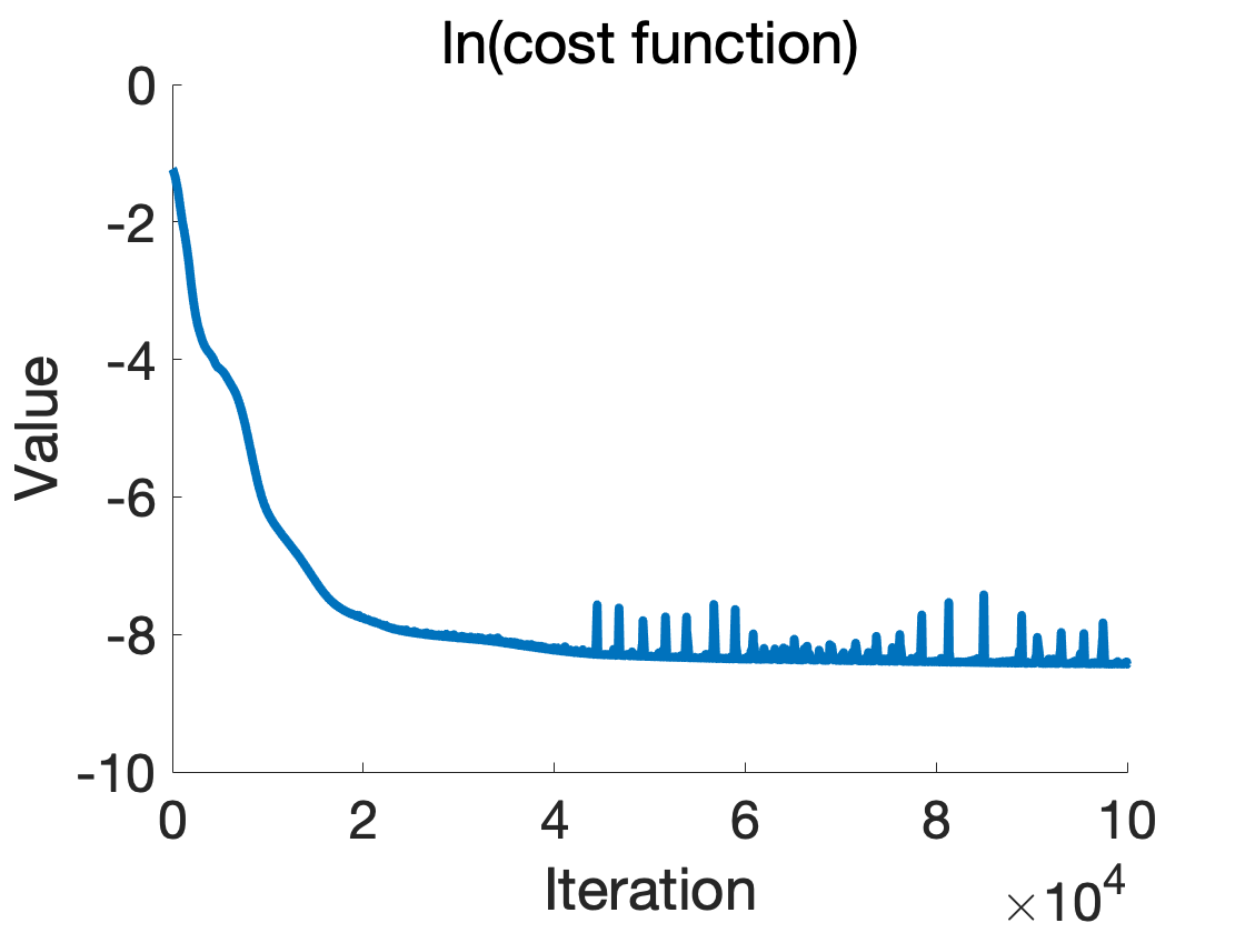
Figure 5. (Left)The design area and boundary conditions of 2d case; (Right)The convergence history of cost function during iterations where time steps = 10−410^{-4}.

There are 2000 points and 500 points randomly sampling in Ω\Omega and Γ\Gamma, respectively. The level of noise δ\delta is set to be zero at first and the discussion of influence of noise is presented in following section 4.3. Fig. 5 (right) shows the convergence history of the cost function and Fig. 6 presents ANN solution and errors between exact solution and neural network approach. To display the depression curve more clearly, we add ln\ln function to the cost function data. It can be observed that the optimization process is stable up to 30000 iteration steps, which verifies the accuracy of ANN for time-independent case in 2D.

Refer to caption
Refer to caption
Figure 6. (Left) The ANN solution to example 2; (Right) the errors between exact and computed solution.

To illustrate the universality of this method, more examples for time-independent case in 2D are given. With same parameters as example 2, we present the following example:

Example 3.

The equation of problem is given as

(4.3) {Δ​u​(𝐱)=0𝐱inΩu⁡(𝐱)=ln⁡((x1−1)2+(x2−1)2)𝐱onΓ∂u⁡(𝐱)∂𝐧=[2​(x1−1)(x1−1)2+(x2−1)2,2​(x2−1)(x1−1)2+(x2−1)2]∗𝐧𝐱onΓ\begin{cases}\Delta u(\mathbf{x})=0&\mathbf{x}\ \ $in$\ \ \Omega\\ u(\mathbf{x})=\ln\left(\sqrt{(x_{1}-1)^{2}+(x_{2}-1)^{2}}\right)&\mathbf{x}\ \ $on$\ \ \Gamma\\ \frac{\partial u(\mathbf{x})}{\partial\mathbf{n}}=[\frac{2(x_{1}-1)}{(x_{1}-1)^{2}+(x_{2}-1)^{2}},\frac{2(x_{2}-1)}{(x_{1}-1)^{2}+(x_{2}-1)^{2}}]*\mathbf{n}&\mathbf{x}\ \ $on$\ \ \Gamma\end{cases}

where domain Ω\Omega and boundary Γ\Gamma is given in Fig. 7(Left).

Refer to caption
Refer to caption
Figure 7. (Left)The design area and boundary conditions of 2d case; (Right)The convergence history of cost function during iteration where steps = 10−410^{-4}.

The level of noise δ\delta is set to be %1\%1. Fig. 7 (Right) shows the convergence history of the cost function, and errors between exact and computed solution are presented in Fig. 8. As the above results show, ANN method for Cauchy inverse problem of time-independent case is worked on 2D. Higher spatial dimensions cases are considered in the following examples.

Refer to caption
Refer to caption
Figure 8. (Left) The ANN solution to example 3; (Right) the errors between exact and computed solution.
Example 4 (3D case).

The equation of 3D case is given as

(4.4) {Δ​u​(𝐱)=0𝐱inΩu⁡(𝐱)=sinh⁡(2​x1)​sin⁡(x2)​sin⁡(x3)𝐱onΓ∂u⁡(𝐱)∂𝐧=∇(sinh(2x1)sin(x2)sin(x3))∗𝐧𝐱onΓ\begin{cases}\Delta u(\mathbf{x})=0&\mathbf{x}\ \ $in$\ \ \Omega\\ u(\mathbf{x})=\sinh(\sqrt{2}x_{1})\sin(x_{2})\sin(x_{3})&\mathbf{x}\ \ $on$\ \ \Gamma\\ \frac{\partial u(\mathbf{x})}{\partial\mathbf{n}}=\nabla\left(\sinh(\sqrt{2}x_{1})\sin(x_{2})\sin(x_{3})\right)*\mathbf{n}&\mathbf{x}\ \ $on$\ \ \Gamma\end{cases}

Let domain Ω\Omega be (x1−0.5)2+(x2−0.5)2+(x3−0.5)2<0.25(x_{1}-0.5)^{2}+(x_{2}-0.5)^{2}+(x_{3}-0.5)^{2}<0.25 and boundary Γ\Gamma be (x1−0.5)2+(x2−0.5)2+(x3−0.5)2=0.25,x3∈[0,0.25]∪[0.5,0.75](x_{1}-0.5)^{2}+(x_{2}-0.5)^{2}+(x_{3}-0.5)^{2}=0.25,x_{3}\in[0,0.25]\cup[0.5,0.75].

There are 10000 points and 2500 randomly sampling in Ω\Omega and Γ\Gamma, respectively. The structure of ANN is chosen with layers [3,120,20,14,12,10,1][3,120,20,14,12,10,1] and level of noise δ\delta is set to be %1\%1. Fig. 9(a) shows the convergence history of the cost function and errors between exact function and computed solution on edges are displayed in Fig. 9(b). We choose five sections of Ω\Omega and the results are presented in Tab. 2.

Refer to caption
(a) Cost Function
Refer to caption
(b) Edge Error
Figure 9. (a) the convergence history of example 4 and (b) the errors in the edges where step = 5×10−45\times 10^{-4}
x3=0.8536x_{3}=0.8536 x3=0.75x_{3}=0.75 x3=0.5x_{3}=0.5 x3=0.25x_{3}=0.25
exact solution [Uncaptioned image] [Uncaptioned image] [Uncaptioned image] [Uncaptioned image]
errors [Uncaptioned image] [Uncaptioned image] [Uncaptioned image] [Uncaptioned image]
Table 2. The exact solution in one section and errors between exact and computed solution
Example 5 (4-8D cases).

The equation of nD cases are given as

(4.5) {Δ​u​(𝐱)=0𝐱inΩu⁡(𝐱)=x1+x2+⋯+xn𝐱onΓ∂u⁡(𝐱)∂𝐧=∑ini𝐱onΓ\begin{cases}\Delta u(\mathbf{x})=0&\mathbf{x}\ \ $in$\ \ \Omega\\ u(\mathbf{x})=x_{1}+x_{2}+\dots+x_{n}&\mathbf{x}\ \ $on$\ \ \Gamma\\ \frac{\partial u(\mathbf{x})}{\partial\mathbf{n}}=\displaystyle\sum_{i}n_{i}&\mathbf{x}\ \ $on$\ \ \Gamma\end{cases}

Let domain Ω\Omega be x12+x22+⋯+xn2<0.25x_{1}^{2}+x_{2}^{2}+\dots+x_{n}^{2}<0.25 and boundary Γ\Gamma be x12+x22+⋯+xn2=0.25,xn∈[−0.5,−0.25]∪[0,0.25]x_{1}^{2}+x_{2}^{2}+\dots+x_{n}^{2}=0.25,x_{n}\in[-0.5,-0.25]\cup[0,0.25].

There are 10000 and 2500 points randomly sampling in Ω\Omega and Γ\Gamma, respectively. Various dimensions(4-8) are studied to verify the accuracy of ANN method for Cauchy inverse problem. The training ended after 30000 steps, where steps = 10−410^{-4}. Fig. 10 and Table 3 show the corresponding results.

Refer to caption
(a) ln(Cost function)
Refer to caption
(b) ln(Edge error)
Figure 10. The history of cost functions(Left) and edge errors(Right) in 4-8d problems with 49661 test points
4D case 5D case 6D case 7D case 8D case
Training errors 0.0257 0.0237 0.0204 0.0193 0.0142
Test errors 0.0394 0.0302 0.0237 0.0196 0.0153
Table 3. Errors in nd-case after 30000 iterations

As can be seen, there is a good agreement between the present result and the reference solution. The above results show that our method is worked for time-independent Cauchy inverse problem in high spatial dimension cases, and we discover more properties like stability about our method.

4.3. Stability with noisy data and singular domain

The key point of numerical methods for Cauchy inverse problem is to treat the ill-posedness. Numerical experiments with noise on edge data are presented to show the stability of ANN method. The parameters and input data are same as example 2 with two level of noise δ\delta(%1,%0.1\ \%1,\%0.1)., which is illustrated in Tab. 4. We write down the history of cost function after 100000 iterations with noise %1\%1. As can be seen, computed solution will always be convergent with some noise, illustrating that ANN method for Cauchy inverse problem is a good method to deal with ill-posedness.

(%0.1)(\%0.1) noise [Uncaptioned image] [Uncaptioned image] [Uncaptioned image]
(%1)(\%1) noise [Uncaptioned image] [Uncaptioned image] [Uncaptioned image]
Table 4. (Left)errors between exact and computed solution;(Middle)The convergence history of cost function;(Right)edge error between exact and computed solution during iterations

Moreover, it is well-known that some method for Cauchy inverse problem is sensitive with singular area, and the following example 6 will show the sensitivity about ANN method on a singular area.

Example 6 (domain with singularity).

The equation of such problem is given as

(4.6) {Δ​u​(𝐱)=0𝐱inΩu⁡(𝐱)=ex1​s​i​n​(x2)𝐱onΓ∂u⁡(𝐱)∂𝐧=[ex1​s​i​n​(x2),ex1​c​o​s​(x2)]∗𝐧𝐱onΓ\begin{cases}\Delta u(\mathbf{x})=0&\mathbf{x}\ \ $in$\ \ \Omega\\ u(\mathbf{x})=e^{x_{1}}sin(x_{2})&\mathbf{x}\ \ $on$\ \ \Gamma\\ \frac{\partial u(\mathbf{x})}{\partial\mathbf{n}}=[e^{x_{1}}sin(x_{2}),e^{x_{1}}cos(x_{2})]*\mathbf{n}&\mathbf{x}\ \ $on$\ \ \Gamma\end{cases}

We choose a singular domain Ω\Omega and boundary Γ\Gamma which is displayed in Fig. 11(Left).

There are 3000 and 1000 points randomly sampling in Ω\Omega and Γ\Gamma, respectivily. Let us choose the same structure of neural networks as example 2. The level of noise δ\delta is set to be %1\%1. Fig. 11(Right) shows the convergence history of the cost function and errors between exact and computed solution are presented in Fig. 12.

Refer to caption
Refer to caption
Figure 11. (Left)The design area and boundary conditions of example 6; (Right)The convergence history of cost function during iteration where steps = 5×10−45\times 10^{-4}.
Refer to caption
Refer to caption
Figure 12. (Left) The ANN solution to example 2; (Right) the errors between exact and computed solution.

Graphically, there is a good agreement between the numerical and exact solutions, showing that ANN method for Cauchy inverse problem is insensitive with singular area. Moreover, the stability of it is verified.

4.4. The influence of depth and width of networks

The influence of structures of ANN is an important issue which many researchers concern, at last we did some experiments on different hidden layers and neurons to discover it. Firstly five neural networks with different hidden layers are tested with steps =10−4=10^{-4} and 30000 iterations. Fig. 13(Right) shows the corresponding cost function during iterations and Tab. 5 shows errors(with training and testing) of five different hidden layers after 30000 iterations. As can be seen, the values of cost function decent faster with the parameters grows, and networks with more neurons and hidden layers have better approximation to the solution of PDEs, which satisfied theorems in section 3. Secondly the influence of multi and single layers with same amounts of parameters is also tested with 30000 iterations. The result is displayed in Table. 6, illustrating that approximation of multi hidden layers networks is always better than single hidden layers with same amount of parameters. It is worth to mention that when the neurons of one layer are too large(like 2968 parameters in Table 6), the method can not convergent with some initial 𝐰\mathbf{w} and 𝐛\mathbf{b} because of the value of sigmoid function will always approach to 11.

numbers of hidden layers 1 2 3 4 5
Cost Function value 0.1118 0.04897 0.02745 0.01484 0.002148
Test errors (10510^{5} points) 0.08950 0.07075 0.06495 0.06301 0.03483
Table 5. The cost function and test errors after 30000 iterations
Refer to caption
Refer to caption
Figure 13. (Left)The errors between exact and computed solution during iteration; (Right)The convergence history of cost function during iteration where steps = 10−410^{-4}.
Numbers of parameters 10 120 288 568 2968
Single hidden layer case 0.1118 0.1053 0.0947 0.0705 do not convergent
Multi hidden layer case 0.1118 0.04897 0.02745 0.01484 0.002148
Table 6. The cost function value of single and multi hidden layers after 30000 iterations

With above numerical examples, we can conclude that ANN method for Cauchy inverse problem with multi-hidden layers is a stable method on various aspects, including well-posedness with noise on boundary and insensitivity on singular area.

5. Conclusions

We have investigated an artificial neural network approximation for solving Cauchy inverse problem. The inputs of network come from physical models, including the initial and boundary datas with noise, rather than any exact or experiment solutions. Denseness and m-denseness of networks are extended to multi-hidden layers in this paper, so that we can prove the equivalence between Cauchy inverse problem and its ANN approximation. Various numerical examples show that our method is effective for both time-dependent and time-independent cases. It is worth noting that ANN methods for Cauchy inverse problem have some stable properties, such as approaching data with noise δ\delta, solving high-dimension cases with lower computational cost and being insensitive on a singular domain. Moreover, the influence about the number of layers and neurons with neural network are also discovered by numerical examples that networks with more hidden layers have better performance.

In addition, it would be of interest to extend neural network method into other inverse problem or parameter design problem. Otherwise, more novel structures and some convergence analysis of deep learning for solving PDE inverse problems is also an important question. We leave these questions for future work.

Appendix

In the appendix we introduce some computation of the derivation and back propagation based on the chain rule. Artificial neural network can be considered as an approximated function of input data. As is known that operator ℒ\mathcal{L} can be represented by nt​hn_{th}-order derivations of space Ω\Omega. At first, let us compute some derivations of ANN.

Appendix A Back propagation of nt​hn_{th}-order derivations with ANN

A.1. Back propagation with ANN

Back propagation of 0-order derivation is the original backpropagation with ANN. The back propagation with 0-order derivation(∂𝐲L+1∂𝐰1,∂𝐲L+1∂𝐛l\frac{\partial\mathbf{y}^{L+1}}{\partial\mathbf{w}^{1}},\frac{\partial\mathbf{y}^{L+1}}{\partial\mathbf{b}^{l}}) can be computed by taking derivatives of 𝐳l\mathbf{z}^{l} and yly^{l}. Following the chain rule, we know that

(A.1) ∂𝐲L+1∂𝐰l=∂𝐲L+1∂𝐳l∗∂𝐳l∂𝐰l=∂𝐲L+1∂𝐳l∗𝐲l−1,∂𝐲L+1∂𝐛l=∂𝐲L+1∂𝐳l∗∂𝐳l∂𝐛l=∂𝐲L+1∂𝐳l.\begin{split}\frac{\partial\mathbf{y}^{L+1}}{\partial\mathbf{w}^{l}}&=\frac{\partial\mathbf{y}^{L+1}}{\partial\mathbf{z}^{l}}*\frac{\partial\mathbf{z}^{l}}{\partial\mathbf{w}^{l}}=\frac{\partial\mathbf{y}^{L+1}}{\partial\mathbf{z}^{l}}*\mathbf{y}^{l-1},\\ \frac{\partial\mathbf{y}^{L+1}}{\partial\mathbf{b}^{l}}&=\frac{\partial\mathbf{y}^{L+1}}{\partial\mathbf{z}^{l}}*\frac{\partial\mathbf{z}^{l}}{\partial\mathbf{b}^{l}}=\frac{\partial\mathbf{y}^{L+1}}{\partial\mathbf{z}^{l}}.\end{split}

By defining δl:=∂𝐲L+1∂𝐳l,l=1,2,…,L+1\delta^{l}:=\frac{\partial\mathbf{y}^{L+1}}{\partial\mathbf{z}^{l}},l=1,2,\dots,L+1, equation (2) yields that

δL+1=σL+1′​(𝐳L+1),δl=(𝐰l+1)T∗δl+1⊙σl′(𝐳l),l=1,2,…,L;\begin{split}&\delta^{L+1}=\sigma_{L+1}^{\prime}(\mathbf{z}^{L+1}),\\ &\delta^{l}=\left(\mathbf{w}^{l+1}\right)^{T}*\delta^{l+1}\odot\sigma_{l}^{\prime}({\mathbf{z}^{l}}),\ \ \ l=1,2,\dots,L;\end{split}

where ⊙\odot represent multiplication by corresponding elements of two vectors.

A.2. Back propagation of 1-order derivation with ANN

Assume that input 𝐱∈Ω×𝒯⊂ℝd×ℝ1\mathbf{x}\in\Omega\times\mathcal{T}\subset\mathbb{R}^{d}\times\mathbb{R}^{1}, the back propagation of 1-order derivation (∂2𝐲L+1∂𝐰1​∂xi,∂2𝐲L+1∂𝐛l​∂xi\frac{\partial^{2}\mathbf{y}^{L+1}}{\partial\mathbf{w}^{1}\partial x_{i}},\frac{\partial^{2}\mathbf{y}^{L+1}}{\partial\mathbf{b}^{l}\partial x_{i}}) can be obtained in the following equations:

(A.2) ∂2𝐲L+1∂𝐱i​∂𝐰l\displaystyle\frac{\partial^{2}\mathbf{y}^{L+1}}{\partial\mathbf{x}_{i}\partial\mathbf{w}^{l}} =\displaystyle= ∂δl∂𝐱i∗(𝐲l−1)T+δl∗∂(𝐲l−1)T∂𝐱i\displaystyle\frac{\partial\delta^{l}}{\partial\mathbf{x}_{i}}*(\mathbf{y}^{l-1})^{T}+\delta^{l}*\frac{\partial(\mathbf{y}^{l-1})^{T}}{\partial\mathbf{x}_{i}}
(A.3) ∂2𝐲L+1∂𝐱i​∂𝐛l\displaystyle\frac{\partial^{2}\mathbf{y}^{L+1}}{\partial\mathbf{x}_{i}\partial\mathbf{b}^{l}} =\displaystyle= ∂δl∂𝐱i,\displaystyle\frac{\partial\delta^{l}}{\partial\mathbf{x}_{i}},

where ∂δl∂𝐱i\frac{\partial\delta^{l}}{\partial\mathbf{x}_{i}} can be computed as

∂δL+1∂𝐱i=σL+1′′​(𝐳L+1)⊙∂𝐳L+1∂xi∂δl∂𝐱i=(𝐰l+1)T∗∂δl+1∂xi⊙σl′​(𝐳l)+(𝐰l+1)T∗δl+1⊙σl′′​(𝐳l)⊙∂𝐳l∂xi\begin{split}\frac{\partial\delta^{L+1}}{\partial\mathbf{x}_{i}}&=\sigma_{L+1}^{\prime\prime}(\mathbf{z}^{L+1})\odot\frac{\partial\mathbf{z}^{L+1}}{\partial x_{i}}\\ \frac{\partial\delta^{l}}{\partial\mathbf{x}_{i}}&=\left(\mathbf{w}^{l+1}\right)^{T}*\frac{\partial\delta^{l+1}}{\partial x_{i}}\odot\sigma_{l}^{\prime}({\mathbf{z}^{l}})+\left(\mathbf{w}^{l+1}\right)^{T}*\delta^{l+1}\odot\sigma_{l}^{\prime\prime}({\mathbf{z}^{l}})\odot\frac{\partial\mathbf{z}^{l}}{\partial x_{i}}\end{split}

The analytic formula of ∂𝐲l∂xi\frac{\partial\mathbf{y}^{l}}{\partial x_{i}} and ∂𝐳l∂xi\frac{\partial\mathbf{z}^{l}}{\partial x_{i}} in the above equations can be represented one by one with layers as:

∂𝐳1∂xi=𝐰1∂𝐳l+1∂xi=𝐰l+1∗∂𝐳l∂xi⊙σl′​(𝐳l)∂𝐲l∂xi=∂𝐳l∂xi⊙σl′​(𝐳l)\begin{split}&\frac{\partial\mathbf{z}^{1}}{\partial x_{i}}=\mathbf{w}^{1}\\ &\frac{\partial\mathbf{z}^{l+1}}{\partial x_{i}}=\mathbf{w}^{l+1}*\frac{\partial\mathbf{z}^{l}}{\partial x_{i}}\odot\sigma_{l}^{\prime}(\mathbf{z}^{l})\\ &\frac{\partial\mathbf{y}^{l}}{\partial x_{i}}=\frac{\partial\mathbf{z}^{l}}{\partial x_{i}}\odot\sigma_{l}^{\prime}(\mathbf{z}^{l})\end{split}

Moreover, when Ω⊂ℝd,d>3\Omega\subset\mathbb{R}^{d},d>3, it’s convenient to compute with matrix form. Before that we introduce some notations at first.

For a vector 𝐟=[f1,f2,…,fm]\mathbf{f}=[f_{1},f_{2},\dots,f_{m}], the Jacobi matrix of 𝐟\mathbf{f} is defined as

G⁡(𝐟)=[∂f1∂x1∂f1∂x2…∂f1∂xd∂f1∂t∂f2∂x1∂f2∂x2…∂f2∂xd∂f2∂t⋱∂fm∂x1∂fm∂x2…∂fm∂xd∂fm∂t]G(\mathbf{f})=\begin{bmatrix}\frac{\partial f_{1}}{\partial x_{1}}&\frac{\partial f_{1}}{\partial x_{2}}&\dots&\frac{\partial f_{1}}{\partial x_{d}}&\frac{\partial f_{1}}{\partial t}\\ \frac{\partial f_{2}}{\partial x_{1}}&\frac{\partial f_{2}}{\partial x_{2}}&\dots&\frac{\partial f_{2}}{\partial x_{d}}&\frac{\partial f_{2}}{\partial t}\\ \vdots&\vdots&\ddots&\vdots\\ \frac{\partial f_{m}}{\partial x_{1}}&\frac{\partial f_{m}}{\partial x_{2}}&\dots&\frac{\partial f_{m}}{\partial x_{d}}&\frac{\partial f_{m}}{\partial t}\end{bmatrix}

and for a vector 𝐮=[u1,u2,…,un]\mathbf{u}=[u_{1},u_{2},\dots,u_{n}], let the diagonal matrices be

d​i​a​g​(𝐮)=[u10…00u2…0⋱00…un]diag(\mathbf{u})=\begin{bmatrix}u_{1}&0&\dots&0\\ 0&u_{2}&\dots&0\\ \vdots&\vdots&\ddots&\vdots\\ 0&0&\dots&u_{n}\end{bmatrix}

With the above definition there obviously establish in matrix form that

(A.4) G⁡(δL+1)=d​i​a​g​(σL+1′′​(𝐳L+1))∗G⁡(𝐳L+1),G⁡(δl)=d​i​a​g​(σl′​(𝐳l))∗(𝐰l+1)T∗G⁡(δl+1)+d​i​a​g​(σl′′​(𝐳l))∗(𝐰l+1)T∗δl+1⊙G⁡(𝐳l),∂δl∂𝐱i=G⁡(δl)​[i],\begin{split}&G(\delta^{L+1})=diag(\sigma_{L+1}^{\prime\prime}(\mathbf{z}^{L+1}))*G(\mathbf{z}^{L+1}),\\ &G(\delta^{l})=diag(\sigma_{l}^{\prime}(\mathbf{z}^{l}))*(\mathbf{w}^{l+1})^{T}*G(\delta^{l+1})+diag(\sigma_{l}^{\prime\prime}(\mathbf{z}^{l}))*(\mathbf{w}^{l+1})^{T}*\delta^{l+1}\odot G(\mathbf{z}^{l}),\\ &\frac{\partial\delta^{l}}{\partial\mathbf{x}_{i}}=G(\delta^{l})[i],\end{split}

where

G⁡(𝐳1)=𝐰1∗Id+1,G(𝐳l)=𝐰l∗diag(σl−1(𝐳l−1))∗G(𝐳l−1),l=2,3,…,L+1G(𝐲l)=diag(σl′(𝐳l))∗G(𝐳l),l=1,2,…,L+1\begin{split}&G(\mathbf{z}^{1})=\mathbf{w}^{1}*I_{d+1},\\ &G(\mathbf{z}^{l})=\mathbf{w}^{l}*diag(\sigma_{l-1}(\mathbf{z}^{l-1}))*G(\mathbf{z}^{l-1}),\ \ l=2,3,\dots,L+1\\ &G(\mathbf{y}^{l})=diag(\sigma_{l}^{\prime}(\mathbf{z}^{l}))*G(\mathbf{z}^{l}),\ \ l=1,2,\dots,L+1\end{split}

where IdI_{d} is the d×dd\times d identity matrix.

A.3. Back propagation with 2-order derivation of ANN

Assume the input 𝐱∈Ω×𝒯⊂ℝd×ℝ1\mathbf{x}\in\Omega\times\mathcal{T}\subset\mathbb{R}^{d}\times\mathbb{R}^{1}, and back propagation of 2-order derivation (∂3𝐲L+1∂𝐰1​∂2xi,∂3𝐲L+1∂𝐛l​∂2xi\frac{\partial^{3}\mathbf{y}^{L+1}}{\partial\mathbf{w}^{1}\partial^{2}x_{i}},\frac{\partial^{3}\mathbf{y}^{L+1}}{\partial\mathbf{b}^{l}\partial^{2}x_{i}}) can be obtained in the following equations:

(A.5) ∂3𝐲L+1∂𝐰1​∂2xi=∂2δl∂xi2∗(𝐲l−1)T+2​∂δl∂xi∗∂(𝐲l−1)T∂xi+δl∗∂2(𝐲l−1)T∂xi2∂3𝐲L+1∂𝐛l​∂2xi=∂2δl∂xi2,\begin{split}\frac{\partial^{3}\mathbf{y}^{L+1}}{\partial\mathbf{w}^{1}\partial^{2}x_{i}}&=\frac{\partial^{2}\delta^{l}}{\partial x_{i}^{2}}*(\mathbf{y}^{l-1})^{T}+2\frac{\partial\delta^{l}}{\partial x_{i}}*\frac{\partial(\mathbf{y}^{l-1})^{T}}{\partial x_{i}}+\delta^{l}*\frac{\partial^{2}(\mathbf{y}^{l-1})^{T}}{\partial x_{i}^{2}}\\ \frac{\partial^{3}\mathbf{y}^{L+1}}{\partial\mathbf{b}^{l}\partial^{2}x_{i}}&=\frac{\partial^{2}\delta^{l}}{\partial x_{i}^{2}},\end{split}

where ∂2δl∂xi2\frac{\partial^{2}\delta^{l}}{\partial x_{i}^{2}} can be computed as

∂2δL+1∂xi2=σL+1′′′​(𝐳L+1)⊙(∂𝐳L+1∂xi)2∂2δl∂xi2=(𝐰l+1)T∗(∂2δl+1∂xi2⊙σl′​(𝐳l)+2​∂δl+1∂xi⊙σl′′​(𝐳l)⊙∂𝐳l∂xi)+(𝐰l+1)T∗δl⊙(σl′′′(𝐳l)⊙(∂𝐳l∂xi)+σl′′(𝐳l)⊙∂2𝐳l∂xi2)\begin{split}\frac{\partial^{2}\delta^{L+1}}{\partial x_{i}^{2}}&=\sigma_{L+1}^{\prime\prime\prime}(\mathbf{z}^{L+1})\odot\left(\frac{\partial\mathbf{z}^{L+1}}{\partial x_{i}}\right)^{2}\\ \frac{\partial^{2}\delta^{l}}{\partial x_{i}^{2}}&=(\mathbf{w}^{l+1})^{T}*\left(\frac{\partial^{2}\delta^{l+1}}{\partial x_{i}^{2}}\odot\sigma_{l}^{\prime}(\mathbf{z}^{l})+2\frac{\partial\delta^{l+1}}{\partial x_{i}}\odot\sigma_{l}^{\prime\prime}(\mathbf{z}^{l})\odot\frac{\partial\mathbf{z}^{l}}{\partial x_{i}}\right)\\ &+(\mathbf{w}^{l+1})^{T}*\delta^{l}\odot\left(\sigma_{l}^{\prime\prime\prime}(\mathbf{z}^{l})\odot\left(\frac{\partial\mathbf{z}^{l}}{\partial x_{i}}\right)+\sigma_{l}^{\prime\prime}(\mathbf{z}^{l})\odot\frac{\partial^{2}\mathbf{z}^{l}}{\partial x_{i}^{2}}\right)\end{split}

The analytic formula of ∂2𝐲l∂xi2\frac{\partial^{2}\mathbf{y}^{l}}{\partial x^{2}_{i}} and ∂2𝐳l∂xi2\frac{\partial^{2}\mathbf{z}^{l}}{\partial x^{2}_{i}} in the above euqations can be represented one by one with layers:

∂2𝐳1∂xi2\displaystyle\frac{\partial^{2}\mathbf{z}^{1}}{\partial x^{2}_{i}} =\displaystyle= 0\displaystyle 0
∂2𝐳l+1∂xi2\displaystyle\frac{\partial^{2}\mathbf{z}^{l+1}}{\partial x^{2}_{i}} =\displaystyle= 𝐰l+1∗(∂2𝐳l∂xi2⊙σl′​(𝐳l)+(∂𝐳l∂xi)2⊙σl′′​(𝐳l))\displaystyle\mathbf{w}^{l+1}*\left(\frac{\partial^{2}\mathbf{z}^{l}}{\partial x_{i}^{2}}\odot\sigma_{l}^{\prime}(\mathbf{z}^{l})+\left(\frac{\partial\mathbf{z}^{l}}{\partial x_{i}}\right)^{2}\odot\sigma_{l}^{\prime\prime}(\mathbf{z}^{l})\right)
∂2𝐲l∂xi2\displaystyle\frac{\partial^{2}\mathbf{y}^{l}}{\partial x^{2}_{i}} =\displaystyle= ∂2𝐳l∂xi2⊙σl′​(𝐳l)+(∂𝐳l∂xi)2⊙σl′′​(𝐳l)\displaystyle\frac{\partial^{2}\mathbf{z}^{l}}{\partial x_{i}^{2}}\odot\sigma_{l}^{\prime}(\mathbf{z}^{l})+\left(\frac{\partial\mathbf{z}^{l}}{\partial x_{i}}\right)^{2}\odot\sigma_{l}^{\prime\prime}(\mathbf{z}^{l})

Moreover, when Ω⊂ℝd,d>3\Omega\subset\mathbb{R}^{d},d>3, it’s convenient to compute with matrix form. We introduce some notations at first.

For a vector 𝐮\mathbf{u}, G2​(𝐮)G^{2}(\mathbf{u}) is defined as:

G2​(𝐮)=[∂2u1∂x12∂2u1∂x22…,∂2u1∂xd2∂2u2∂x12∂2u2∂x22…,∂2u2∂xd2⋱∂2un∂x12∂2un∂x22…,∂2un∂xd2]G^{2}(\mathbf{u})=\begin{bmatrix}\frac{\partial^{2}u_{1}}{\partial x_{1}^{2}}&\frac{\partial^{2}u_{1}}{\partial x_{2}^{2}}&\dots,&\frac{\partial^{2}u_{1}}{\partial x_{d}^{2}}\\ \frac{\partial^{2}u_{2}}{\partial x_{1}^{2}}&\frac{\partial^{2}u_{2}}{\partial x_{2}^{2}}&\dots,&\frac{\partial^{2}u_{2}}{\partial x_{d}^{2}}\\ \vdots&\vdots&\ddots&\vdots\\ \frac{\partial^{2}u_{n}}{\partial x_{1}^{2}}&\frac{\partial^{2}u_{n}}{\partial x_{2}^{2}}&\dots,&\frac{\partial^{2}u_{n}}{\partial x_{d}^{2}}\end{bmatrix}

The matrix form of 2-order derivations are shown as

(A.6) G2​(δL+1)=d​i​a​g​(σL+1(3))∗(∇𝐳L+1⊙∇𝐳L+1)+d​i​a​g​(σL+1′′​(𝐳L+1))∗G2​(𝐳L+1)\displaystyle G^{2}(\delta^{L+1})=diag(\sigma_{L+1}^{(3)})*(\nabla\mathbf{z}^{L+1}\odot\nabla\mathbf{z}^{L+1})+diag(\sigma_{L+1}^{\prime\prime}(\mathbf{z}^{L+1}))*G^{2}(\mathbf{z}^{L+1})
(A.7) G2​(δl)=d​i​a​g​(σl′​(𝐳l))∗(𝐰l+1)T∗G2​(δl+1)+diag(σl′′(𝐳l))∗(𝐰l+1)T∗(2∇δl+1)⊙∇𝐳l+d​i​a​g​(σl(3)​(𝐳l))∗(𝐰l+1)T∗δl+1⊙(∇𝐳l⊙∇𝐳l)+d​i​a​g​(σl′′​(𝐳l))∗(𝐰l+1)T∗δl+1⊙J⁡(𝐳l),l=1,2,…,L\displaystyle\begin{split}G^{2}(\delta^{l})=&diag(\sigma_{l}^{\prime}(\mathbf{z}^{l}))*(\mathbf{w}^{l+1})^{T}*G^{2}(\delta^{l+1})+\\ &diag(\sigma_{l}^{\prime\prime}(\mathbf{z}^{l}))*(\mathbf{w}^{l+1})^{T}*(2\nabla\delta^{l+1})\odot\nabla\mathbf{z}^{l}+\\ &diag(\sigma_{l}^{(3)}(\mathbf{z}^{l}))*(\mathbf{w}^{l+1})^{T}*\delta^{l+1}\odot(\nabla\mathbf{z}^{l}\odot\nabla\mathbf{z}^{l})+\\ &diag(\sigma_{l}^{\prime\prime}(\mathbf{z}^{l}))*(\mathbf{w}^{l+1})^{T}*\delta^{l+1}\odot J(\mathbf{z}^{l}),\ \ l=1,2,\dots,L\end{split}
(A.8) ∂2δl∂xi2=G2​(δl)​[i],\displaystyle\frac{\partial^{2}\delta^{l}}{\partial x_{i}^{2}}=G^{2}(\delta^{l})[i],

There obviously establishes following equation for G2​(𝐳l)G^{2}(\mathbf{z}^{l}) and G2​(𝐳l)G^{2}(\mathbf{z}^{l}):

G2​(𝐳1)=𝐰1∗Od+1,G2​(𝐳l)=𝐰l∗(d​i​a​g​(σl−1′′​(𝐳l−1))∗(∇𝐳l−1⊙∇𝐳l−1)+d​i​a​g​(σl−1′​(𝐳l−1))∗G2​(𝐳l−1)),OPENG2​(𝐲l)=d​i​a​g​(σl′′​(𝐳l))∗(∇𝐳l⊙∇𝐳l)+d​i​a​g​(σl′​(𝐳l))∗G2​(𝐳L+1)),\begin{split}&G^{2}(\mathbf{z}^{1})=\mathbf{w}^{1}*O_{d+1},\\ &G^{2}(\mathbf{z}^{l})=\mathbf{w}^{l}*(diag(\sigma_{l-1}^{\prime\prime}(\mathbf{z}^{l-1}))*(\nabla\mathbf{z}^{l-1}\odot\nabla\mathbf{z}^{l-1})+diag(\sigma_{l-1}^{\prime}(\mathbf{z}^{l-1}))*G^{2}(\mathbf{z}^{l-1})),\\ &G^{2}(\mathbf{y}^{l})=diag(\sigma_{l}^{\prime\prime}(\mathbf{z}^{l}))*(\nabla\mathbf{z}^{l}\odot\nabla\mathbf{z}^{l})+diag(\sigma_{l}^{\prime}(\mathbf{z}^{l}))*G^{2}(\mathbf{z}^{L+1})),\end{split}

where OdO_{d} is the zero matrix of dimension d×dd\times d.

Appendix B The analytic formula of back propagation for Cauchy inverse problem

We use the result and notation in the last appendix A. Firstly, we show the analytic formula of back propagation for problem (1.2), and problem (1.1) is similar.

The back propagation for Dirichlet boundary condition and initial condition can be easily obtained in equation (A.1). Neumann boundary condition and the state equation is considered with problem (1.2).

B.1. back propagation for Neumann boundary condition

We know that for time dependent problem, there establish that

(B.1) G⁡(𝐲L+1)=[∂𝐲L+1∂x1∂𝐲L+1∂x2…∂𝐲L+1∂xd∂𝐲L+1∂t]G(\mathbf{y}^{L+1})=\begin{bmatrix}\frac{\partial\mathbf{y}^{L+1}}{\partial x_{1}}&\frac{\partial\mathbf{y}^{L+1}}{\partial x_{2}}&\dots&\frac{\partial\mathbf{y}^{L+1}}{\partial x_{d}}&\frac{\partial\mathbf{y}^{L+1}}{\partial t}\end{bmatrix}

Neumann boundary condition can be represented by

(B.2) ∂𝐲L+1∂𝐧=∇𝐲L+1∗DT(𝐱)=G(𝐲L+1)[1:d]∗DT(𝐱),\frac{\partial\mathbf{y}^{L+1}}{\partial\mathbf{n}}=\nabla\mathbf{y}^{L+1}*D^{T}(\mathbf{x})=G(\mathbf{y}^{L+1})[1:d]*D^{T}(\mathbf{x}),

where D⁡(𝐱)=(β1,β2,…,βd)D(\mathbf{x})=(\beta_{1},\beta_{2},\dots,\beta_{d}) represents the direction at points 𝐱\mathbf{x}. Similarly the back propagation of Neumann boundary condition is shown as following

(B.3) ∂2𝐲L+1∂𝐧​∂𝐰l\displaystyle\frac{\partial^{2}\mathbf{y}^{L+1}}{\partial\mathbf{n}\partial\mathbf{w}^{l}} =\displaystyle= ∂∇𝐲L+1∂𝐰l∗DT​(𝐱)=∇∂𝐲L+1∂𝐰l∗DT​(𝐱),\displaystyle\frac{\partial\nabla\mathbf{y}^{L+1}}{\partial\mathbf{w}^{l}}*D^{T}(\mathbf{x})=\nabla\frac{\partial\mathbf{y}^{L+1}}{\partial\mathbf{w}^{l}}*D^{T}(\mathbf{x}),
(B.4) ∂2𝐲L+1∂𝐧​∂𝐛l\displaystyle\frac{\partial^{2}\mathbf{y}^{L+1}}{\partial\mathbf{n}\partial\mathbf{b}^{l}} =\displaystyle= ∂∇𝐲L+1∂𝐛l∗DT​(𝐱)=∇∂𝐲L+1∂𝐛l∗DT​(𝐱),\displaystyle\frac{\partial\nabla\mathbf{y}^{L+1}}{\partial\mathbf{b}^{l}}*D^{T}(\mathbf{x})=\nabla\frac{\partial\mathbf{y}^{L+1}}{\partial\mathbf{b}^{l}}*D^{T}(\mathbf{x}),

Let s​u​m​(A)sum(A) be the vector whose corresponding element is the sum of AA’s columns, there establishes that

(B.5) ∇∂𝐲L+1∂𝐰l∗DT​(𝐱)=sum(diag(D(𝐱))∗G(δl)[1:d])∗(𝐲l−1)T+δl∗sum(diag(D(𝐱))∗G(𝐲l−1)T[1:d]),\begin{split}\nabla\frac{\partial\mathbf{y}^{L+1}}{\partial\mathbf{w}^{l}}*D^{T}(\mathbf{x})&=sum(diag(D(\mathbf{x}))*G(\delta^{l})[1:d])*(\mathbf{y}^{l-1})^{T}\\ &+\delta^{l}*sum(diag(D(\mathbf{x}))*G(\mathbf{y}^{l-1})^{T}[1:d]),\end{split}
(B.6) ∇∂𝐲L+1∂𝐛l∗DT(𝐱)=sum(diag(D(𝐱))∗G(δl)[1:d]),\nabla\frac{\partial\mathbf{y}^{L+1}}{\partial\mathbf{b}^{l}}*D^{T}(\mathbf{x})=sum(diag(D(\mathbf{x}))*G(\delta^{l})[1:d]),

So that we can compute back propagation for Neumann boundary condition with equation (B.2) to (B.6)

B.2. back propagation for state equation

It is obvious that the term of time(∂𝐲L+1∂t\frac{\partial\mathbf{y}^{L}+1}{\partial t}) in problem (1.2) can be computed directly by equation A.2 and A.3. The more important thing to compute is the back propagation for operator ℒ\mathcal{L}. There are lots of choice for ℒ\mathcal{L} and in this paper we just show the gradient operator ∇\nabla and Laplace operator Δ\Delta. More operator of high order can be computed similar as them.

We know that ∇𝐲L+1=G(𝐲L+1)[1:d]\nabla\mathbf{y}^{L+1}=G(\mathbf{y}^{L+1})[1:d], so that the back propagation can be computed directly by equation (A.2). Then let’s consider the Laplace operator. We know that

(B.7) Δ​𝐲L+1=∑i=1d∂2𝐲L+1∂xi2\Delta\mathbf{y}^{L+1}=\displaystyle\sum_{i=1}^{d}\frac{\partial^{2}\mathbf{y}^{L+1}}{\partial x_{i}^{2}}

Following equation (A.6), there establish Δ𝐮=sum(G2(𝐮)[1:d])\Delta\mathbf{u}=sum(G^{2}(\mathbf{u})[1:d]). Define Gd(𝐮):=G2(𝐮)[1:d]G_{d}(\mathbf{u}):=G^{2}(\mathbf{u})[1:d], then we have the back propagation as

(B.8) ∂Δ​𝐲L+1∂𝐰l=∑i=1d∂3𝐲L+1∂xi2​∂𝐰l=∑i=1d∂2∂xi2​(δl∗(𝐲l−1)T)=(∑i=1d∂2δl∂xi2)∗(𝐲l−1)T+2​∑i=1d∂δl∂xi∗∂(𝐲l−1)T∂xi+δl∗(∑i=1d∂2(𝐲l−1)T∂xi2)=sum(Gd(δl))∗(𝐲l−1)T+2∇δl∗∇(𝐲l−1)T+δl∗sum(GdT(𝐲l−1)))\displaystyle\begin{split}\frac{\partial\Delta\mathbf{y}^{L+1}}{\partial\mathbf{w}^{l}}&=\displaystyle\sum_{i=1}^{d}\frac{\partial^{3}\mathbf{y}^{L+1}}{\partial x_{i}^{2}\partial\mathbf{w}^{l}}\\ &=\sum_{i=1}^{d}\frac{\partial^{2}}{\partial x_{i}^{2}}\left(\delta^{l}*(\mathbf{y}^{l-1})^{T}\right)\\ &=\left(\sum_{i=1}^{d}\frac{\partial^{2}\delta^{l}}{\partial x_{i}^{2}}\right)*(\mathbf{y}^{l-1})^{T}+2\sum_{i=1}^{d}\frac{\partial\delta^{l}}{\partial x_{i}}*\frac{\partial(\mathbf{y}^{l-1})^{T}}{\partial x_{i}}+\delta^{l}*\left(\sum_{i=1}^{d}\frac{\partial^{2}(\mathbf{y}^{l-1})^{T}}{\partial x_{i}^{2}}\right)\\ &=sum(G_{d}(\delta^{l}))*(\mathbf{y}^{l-1})^{T}+2\nabla\delta^{l}*\nabla(\mathbf{y}^{l-1})^{T}+\delta^{l}*sum(G_{d}^{T}(\mathbf{y}^{l-1})))\end{split}
(B.9) ∂Δ​𝐲L+1∂𝐛l=∑i=1d∂3𝐲L+1∂xi2​∂𝐛l=s​u​m​(Gd​(δl)),\displaystyle\begin{split}\frac{\partial\Delta\mathbf{y}^{L+1}}{\partial\mathbf{b}^{l}}&=\displaystyle\sum_{i=1}^{d}\frac{\partial^{3}\mathbf{y}^{L+1}}{\partial x_{i}^{2}\partial\mathbf{b}^{l}}=sum(G_{d}(\delta^{l})),\end{split}

With all the above equation (B.7) to (B.9), we can compute the back propagation for state equation for various operator ℒ\mathcal{L}.

References

References

  • [1] L. P. Aarts and P. van der Veer. Neural network method for solving partial differential equations. Neural Processing Letters, 14(3):261–271, 2001.
  • [2] D. A. amd P. Besala. Uniqueness of solutions of the cauchy problem for parabolic equations. Journal of Mathematical Analysis and Applications, 13:516–526, 1966.
  • [3] F. Berntsson, V. Kozlov, L. Mpinganzima, and B. Turesson. An accelerated alternating procedure for the cauchy problem for the helmholtz equation. Computers and Mathematics with Applications, 68:44–60, 2014.
  • [4] F. Berntsson, V. Kozlov, L. Mpinganzima, and B. Turesson. Iterative tikhonov regularization for the cauchy problem for the helmholtz equation. Computers and Mathematics with Applications, 73:163–172, 2017.
  • [5] L. Bourgeois. A mixed formulation of quasi-reversibility to solve the cauchy problem for laplace’s equation. Inverse Problems, 21(3):1087–1104, 2005.
  • [6] J. R. Cannon and J. Douglas, Jr. The cauchy problem for the heat hquation. SIAM Journal on Numerical Analysis, 4(3):317–336, 1967.
  • [7] G. Carleo and M. Troyer. Solving the quantum many-body problem with artificial neural networks. Science, 355(6325):602–606, 2017.
  • [8] A. Chakib and A. Nachaoui. Convergence analysis for finite element approximation to an inverse cauchy problem. Inverse Problems, 22(4), 2006.
  • [9] X. Cheng, R. Gong, W. Han, and X. Zheng. A novel coupled complex boundary method for solving inverse source problems. Inverse Problems, 30(5):055002, 2014.
  • [10] A. Cimetière, F. Delvare, M. Jaoua, and F. Pons. Solution of the cauchy problem using iterated tikhonov regularization. Inverse Problems, 17(3):553–570, 2001.
  • [11] G. Cybenko. Approximation by superpositions of a sigmoidal function. Mathematics of Control, Signals, and Systems, 2:303–314, 1989.
  • [12] L. Elden. Approximations for a cauchy problem for the heat equation. Inverse Problems, 3(2):263–273, 1987.
  • [13] X. Feng and L. Eldén. Solving a cauchy problem for a 3d elliptic PDE with variable coefficients by a quasi-boundary-value method. Inverse Problems, 30(1):015005, 2013.
  • [14] Y. C. Hon and T. Wei. Backus-gilbert algorithm for the cauchy problem of the laplace equation. Inverse Problems, 17(2):261–271, 2001.
  • [15] K. Hornik. Multilayer feedforward networks are universal approximators. Neural Networks, 2:359–366, 1989.
  • [16] K. Hornik. Approximation capabilities of multilayer feedforward networks. Neural Networks, 4:251–257, 1991.
  • [17] D. N. Hào and D. Lesnic. The cauchy problem for laplace’s equation via the conjugate gradient method. IMA Journal of Applied Mathematics, 65(2):199–217, 2000.
  • [18] V. Isakov. Inverse problem for partial differential equations. Springer-Verlag, New York, 1998.
  • [19] B. Jin and J. Zou. Augmented tikhonov regularization. Inverse Problems, 25(2):025001, 2008.
  • [20] B. Jin and J. Zou. Hierarchical bayesian inference for ill-posed problems via variational method. Journal of Computational Physics, 229:7317–7343, 2010.
  • [21] M. Jourhmane and A. Nachaoui. Convergence of an alternating method to solve the cauchy problem for poisson’s equation. Applicable Analysis, 81(5):1065–1083, 2002.
  • [22] I. Kazufumi and B. Jin. Inverse problem. Tikhonov theory and algorithm. Series on Applied Mathematics, vol. 22, World Scientific, Singapore, 2014.
  • [23] M. Klibanov and F. Santosa. A computational quasi-reversibility method for cauchy problems for laplace’s equation. SIAM Journal on Applied Mathematics, 51(6):1653–1675, 1991.
  • [24] I. E. Lagaris, A. Likas, and D. I. Fotiadis. Artificial neural networks for solving ordinary and partial differential equations. IEEE Transactions on Neural Networks, 9(5):987–1000, 1998.
  • [25] I. E. Lagaris, A. C. Likas, and D. G. Papageorgiou. Neural-network methods for boundary value problems with irregular boundaries. IEEE Transactions on Neural Networks, 11(5):1041–1049, 2000.
  • [26] Q. Li, L. Chen, C. Tai, and W. E. Maximum principle based algorithms for deep learning. Journal of Machine Learning Research, 18(165):1–29, 2018.
  • [27] Z. Long, Y. Lu, and B. Dong. Pde-net 2.0: Learning pdes from data with a numeric-symbolic hybrid deep network. Journal of Computational Physics, 399:108925, 2019.
  • [28] A. Malek and R. S. Beidokhti. Numerical solution for high order differential equations using a hybrid neural network—optimization method. Applied Mathematics and Computation, 183(1):260–271, 2006.
  • [29] L. Marin, L. Elliott, P. Heggs, D. Ingham, D. Lesnic, and X. Wen. An alternating iterative algorithm for the cauchy problem associated to the helmholtz equation. Computer Methods in Applied Mechanics and Engineering, 192(5-6):709–722, 2003.
  • [30] S. Mishra. A machine learning framework for data driven acceleration of computations of differential equations. Mathematics in Engineering, 1(1):118–146, 2018.
  • [31] A. Nachaoui. Numerical linear algebra for reconstruction inverse problems. Journal of Computational and Applied Mathematics, 162(1):147–164, 2004.
  • [32] G. Pang, L. Lu, and G. E. Karniadakis. fpinns: Fractional physics-informed neural networks. SIAM Journal on Scientific Computing, 41(4):A2603–A2626, 2019.
  • [33] H. Qin and T. Wei. Two regularization methods for the cauchy problems of the helmholtz equation. Applied Mathematical Modelling, 34(4):947–967, 2010.
  • [34] T. Qin, K. Wu, and D. Xiu. Data driven governing equations approximation using deep neural networks. Journal of Computational Physics, 395:620–635, 2019.
  • [35] M. Raissia, P. Perdikarisb, and G. Karniadakis. Physics-informed neural networks: A deep learning framework for solving forward and inverse problems involving nonlinear partial differential equations. Journal of Computational Physics, 378:686–707, 2019.
  • [36] H. Reinhardt, H. Han, and D. Hào. Stability and regularization of a discrete approximation to the cauchy problem for laplace’s equation. SIAM Journal on Numerical Analysis, 36(3):890–905, 1999.
  • [37] K. Sakamoto and M. Yamamoto. Initial value/boundary value problems for fractional diffusion-wave equations and applications to some inverse problems. Journal of Mathematical Analysis and Applications, 382:426–447, 2011.
  • [38] J. Sirignano and K. Spiliopoulos. Dgm: A deep learning algorithm for solving partial differential equations. Journal of Computational Physics, 375:1339–1364, 2018.
  • [39] T. Takeuchi and M. Yamamoto. Tikhonov regularization by a reproducing kernel hilbert space for the cauchy problem for an elliptic equation. SIAM Journal on Scientific Computing, 31(1):112–142, 2008.
  • [40] T. Wei, Y. Chen, and J. Liu. A variational-type method of fundamental solutions for a cauchy problem of laplace’s equation. Applied Mathematical Modelling, 37:1039–1053, 2013.
  • [41] D. A. White, W. J. Arrighi, J. Kudo, and S. E. Watts. Multiscale topology optimization using neural network surrogate models. Computer Methods in Applied Mechanics and Engineering, 345(1):1118–1135, 2019.
  • [42] L. Yan and T. Zhou. Adaptive multi-fidelity polynomial chaos approach to bayesian inference in inverse problems. Journal of Computational Physics, 381:110–128, 2019.
  • [43] Y.S.Li and T. Wei. An inverse time-dependent source problem for a time–space fractional diffusion equation. Applied Mathematics and Computation, 336:257–271, 2018.
  • [44] D. Zhang, L. Lu, and G. E. Karniadakis. Quantifying total uncertainty in physics-informed neural networks for solving forward and inverse stochastic problems. Journal of Computational Physics, 399:108925, 2019.
  • [45] Y. Zhang, R. Gong, X. Cheng, and M. Gulliksson. A dynamical regularization algorithm for solving inverse source problems of elliptic partial differential equations. Inverse Problems, 34(6):065001, 2018.