Scalable Gradients for Stochastic Differential Equations
Xuechen Li∗ Ting-Kam Leonard Wong Ricky T. Q. Chen David Duvenaud
Google Research University of Toronto University of Toronto Vector Institute University of Toronto Vector Institute
Abstract
The adjoint sensitivity method scalably computes gradients of solutions to ordinary differential equations. We generalize this method to stochastic differential equations, allowing time-efficient and constant-memory computation of gradients with high-order adaptive solvers. Specifically, we derive a stochastic differential equation whose solution is the gradient, a memory-efficient algorithm for caching noise, and conditions under which numerical solutions converge. In addition, we combine our method with gradient-based stochastic variational inference for latent stochastic differential equations. We use our method to fit stochastic dynamics defined by neural networks, achieving competitive performance on a 50-dimensional motion capture dataset.
1 Introduction
Deterministic dynamical systems can often be modeled by ordinary differential equations (ODEs). The adjoint sensitivity method can efficiently compute gradients of ODE solutions with constant memory cost. This method was well-known in the physics, numerical analysis, and control communities for decades [60, 65, 3, 4]. Recently, it was combined with modern reverse-mode automatic differentiation packages, enabling ODEs with millions of parameters to be fit to data [12] and allowing more flexible density estimation and time series models [23, 72, 32].
Stochastic differential equations (SDEs) generalize ODEs, adding instantaneous noise to their dynamics [55, 78, 77]. They are a natural model for phenomena governed by many small and unobserved interactions, such as motion of molecules in a liquid [8], allele frequencies in a gene pool [15], or prices in a market [79]. Previous attempts on fitting SDEs mostly relied on methods with poor scaling properties. The pathwise approach [22, 89], a form of forward-mode automatic differentiation, scales poorly in time with the number of parameters and states in the model. On the other hand, simply differentiating through the operations of an SDE solver [19] scales poorly in memory.
In this work, we generalize the adjoint method to stochastic dynamics defined by SDEs. We give a simple and practical algorithm for fitting SDEs with tens of thousands of parameters, while allowing the use of high-order adaptive time-stepping SDE solvers. We call this approach the stochastic adjoint sensitivity method.
| Method | Memory | Time |
|---|---|---|
| Forward pathwise [89, 22] | ||
| Backprop through solver [19] | ||
| Stochastic adjoint (ours) |
There are two main difficulties in generalizing the adjoint formulation for ODEs to SDEs. The first is mathematical: SDEs are defined using nonstandard integrals that usually rely on Itô calculus. The adjoint method requires solving the dynamics backwards in time from the end state. However, it is not clear exactly what “running the SDE backwards” means in the context of stochastic calculus, and when it correctly reconstructs the forward trajectory. We address this problem in Section 3, deriving a backward Stratonovich SDE whose dynamics compute the necessary gradient.
The second difficulty is computational: To retrace the steps, one needs to reconstruct the noise sampled on the forward pass, ideally without storing it. In Section 4, we give an algorithm that allows querying a Brownian motion sample at any time point arbitrarily-precisely, while only storing a single random seed.
We combine our adjoint approach with a gradient-based stochastic variational inference scheme for efficiently marginalizing over latent SDE models with arbitrary differentiable likelihoods. This model family generalizes several existing families such as latent ODEs [12, 72], Gaussian state-space models [36, 81], and deep Kalman filters [40], and can naturally handle irregularly-sampled times series and missing observations. We train latent SDEs on toy and real datasets, demonstrating competitive performance compared to existing approaches for dynamics modeling.
2 Background: Stochastic Flows
2.1 Adjoint Sensitivity Method
The adjoint sensitivity method is an efficient approach to solve control problems relying on the adjoint (co-state) system [65]. Chen et al. 2018 used this method to compute the gradient with respect to parameters of a neural ODE, which is a particular model among many others inspired by the theory of dynamical systems [46, 11, 74, 26, 10, 44, 86]. The method, shown in Algorithm 1, is scalable, since the most costly computation is a vector-Jacobian product defining its backwards dynamics. In addition, since the gradient is obtained by solving another ODE, no intermediate computation is stored as in the case of regular backpropagation [73].
2.2 Stochastic Differential Equations
Consider a filtered probability space on which an -dimensional adapted Wiener process (or Brownian motion) is defined. For a fixed terminal time , we denote by the time horizon. We denote the th component of by . Due to space constraint, we refer the read to Appendix 9.1 for more on notation.
A stochastic process can be defined by an Itô SDE
| (2) |
where is the starting state, and and are the drift and diffusion functions, respectively. For ease of presentation, we let in the following unless otherwise stated. Our contributions can be easily generalized to cases where . Here, the second integral on the right hand side of (2) is the Itô stochastic integral [55]. When the coefficients are globally Lipschitz in both the state and time, there exists a unique strong solution to the SDE [55].
2.3 Neural Stochastic Differential Equations
Similar to neural ODEs, one can consider drift and diffusion functions defined by neural networks, a model known as the neural SDE [82, 83, 45, 32].
Among works on neural SDEs, none has enabled an efficient training framework. In particular, Tzen and Raginsky 2019a and Liu et al. 2019 considered computing the gradient by simulating the forward dynamics of an explicit Jacobian matrix. This Jacobian has size of either the square of the number of parameters, or the number of parameters times the number of states, building on the pathwise approach [22, 89]. In contrast, our approach only requires a small number of cheap vector-Jacobian products, independent of the dimension of the parameter and state vectors. These vector-Jacobian products have the same asymptotic time cost as evaluating the drift and diffusion functions, and can be easily computed by modern automatic differentiation libraries [49, 59, 1, 16].
2.4 Backward Stratonovich Integral
Our stochastic adjoint sensitivity method involves stochastic processes running both forward and backward in time. The Stratonovich stochastic integral, due to its symmetry, gives nice expressions for the backward dynamics and is more convenient for our purpose. Our results can also be straightforwardly applied to Itô SDEs, relying on a simple conversion rule (see e.g. [64, Sec. 2]).
Following the treatment of Kunita [41], we introduce the forward and backward Stratonovich integrals. Let be a two-sided filtration, where is the -algebra generated by for such that . For a continuous semimartingale adapted to the forward filtration , the Stratonovich stochastic integral is
| (3) |
where is a partition of the interval , denotes the size of largest segment of the partition, and the limit is to be interpreted in the sense. The Itô integral uses instead the left endpoint rather than the average. In general, the Itô and Stratonovich integrals differ by a term of finite variation.
To define the backward Stratonovich integral, we consider the backward Wiener process defined as that is adapted to the backward filtration . For a continuous semimartingale adapted to the backward filtration, the backward Stratonovich integral is
where is the partition.
2.5 Stochastic Flow of Diffeomorphisms
It is well known that an ODE defines a flow of diffeomorphisms [6]. Here we consider the stochastic analog for the Stratonovich SDE
| (52) |
Throughout the paper, we assume that both and have infinitely many bounded derivatives w.r.t. the state, and bounded first derivatives w.r.t. time, i.e. , and thus the SDE has a unique strong solution. Let be the solution at time when the process is started at at time . Given a realization of the Wiener process, this defines a collection of continuous maps from to itself.
The following theorem shows that these maps are diffeomorphisms (after choosing a suitable modification) and that they satisfy backward SDEs.
Theorem 2.1 ([41, Theorem 3.7.1]).
- (a)
With probability , the collection satisfies the flow property
(53) Moreover, each is a smooth diffeomorphism from to itself. We thus call the stochastic flow of diffeomorphisms generated by the SDE (52).
- (b)
The backward flow satisfies the backward SDE:
for all and such that .
The coefficients in (52) and ((b)) differ by only a negative sign. This symmetry is due to our use of the Stratonovich integral (see Figure 2).
3 Sensitivity via Stochastic Adjoint
We present our main contribution: a stochastic analog of the adjoint sensitivity method for SDEs. We use ((b)) to derive another backward Stratonovich SDE, which we call the stochastic adjoint process. The direct implication is a gradient computation algorithm that works by solving a set of dynamics in reverse time, and relies on cheap vector-Jacobian products without storing any intermediate quantities.
3.1 Stochastic Adjoint Process
The goal is to derive a stochastic adjoint process that can be simulated by evaluating only vector-Jacobian products, where is a scalar loss of the terminal state from the forward flow .
We first derive a backward SDE for the process , assuming that follows the inverse flow from a deterministic end state that does not depend on the realized Wiener process (Lemma 3.1). We then extend to the case where is obtained by the forward flow starting from a deterministic initial state (Theorem 3.2). This latter part is unconventional, and the resulting value cannot be interpreted as the solution to a backward SDE anymore due to loss of adaptedness. Instead, we will formulate the result with the Itô map [69]. Finally, it is straightforward to extend the state to include parameters of the drift and diffusion functions such that the desired gradient can be obtained for stochastic optimization; we comment on this step in Section 3.3.
We first present the SDE for the Jacobian matrix of the backward flow.
Lemma 3.1 (Dynamics of ).
The proof included in Appendix 9.2 relies on Itô’s lemma in the Stratonovich form [41, Theorem 2.4.1]. We stress that this lemma considers only the case where the endpoint is fixed and deterministic.
Now, we extend to the case where the endpoint is not deterministic, but rather computed from the forward flow. To achieve this, we compose the state process and the loss function. Consider . The chain rule gives . Let
Note that . Since is a constant, satisfies the augmented backward SDE system
Since the drift and diffusion functions of this augmented system are , the system has a unique strong solution. Let and . Since (3.1) admits a strong solution, we may write
where denotes the path of the Wiener process and
| (166) |
is a deterministic measurable function (the Itô map) [69, Chapter V, Definition 10.9]. Intuitively, can be thought as a black box that computes the solution to the backward SDE system (3.1) given the position at time and the realized Wiener process sample. Similarly, we let be the solution map for the forward flow (52). The next theorem follows immediately from (3.1) and the definition of .
Theorem 3.2.
For -almost all , we have
| (167) |
where .
Proof.
This is a consequence of composing and (3.1). ∎
3.2 Numerical Approximation
In practice, we compute solutions to SDEs with numerical solvers and , where denotes the mesh size of a fixed grid. The approximate algorithm thus outputs . The following theorem provides sufficient conditions for convergence.
Theorem 3.3.
Suppose the schemes and satisfy the following conditions: (i) and in probability as , and (ii) for any , we have in probability as . Then, for any starting point of the forward flow, we have
| (168) |
in probability as .
See Appendix 9.3 for the proof. Usual schemes such as the Euler-Maruyama scheme (more generally Itô-Taylor schemes) converge pathwise (i.e. almost surely) from any fixed starting point [38] and satisfies . While is strong, we note that the SDEs considered here have smooth coefficients, and thus their solutions enjoy nice regularity properties in the starting position. Therefore, it is reasonable to expect that the corresponding numerical schemes to also behave nicely as a function of both the mesh size and the starting position. To the best of our knowledge, this property is not considered at all in the literature on numerical methods for SDEs (where the initial position is fixed), but is crucial in the proof of Theorem 3.3. In Appendix 9.4, we prove that condition holds for the Euler-Maruyama scheme. Detailed analysis for other schemes is beyond the scope of this paper.
3.3 The Algorithm
So far we have derived the gradient of the loss with respect to the initial state. We can extend these results to give gradients with respect to parameters of the drift and diffusion functions by treating them as an additional part of the state whose dynamics has zero drift and diffusion. We summarize this in Algorithm 2, assuming access only to a black-box solver sdeint. All terms in the augmented dynamics, such as and can be cheaply evaluated by calling and , respectively.
Difficulties with non-diagonal diffusion.
In principle, we can simulate the forward and backward adjoint dynamics with any high-order solver of choice. However, for general matrix-valued diffusion functions , to obtain a numerical solution with strong order11 1 A numerical scheme is of strong order if for all , where and are respectively the coupled true solution and numerical solution, and are respectively the iteration index and step size such that , and is independent of . beyond , we need to simulate multiple integrals of the Wiener process such as , . These random variables are difficult to simulate and costly to approximate [87].
Fortunately, if we restrict our SDE to have diagonal noise, then even though the backward SDE for the stochastic adjoint will not in general have diagonal noise, it will satisfy a commutativity property [70]. In that case, we can safely adopt certain numerical schemes of strong order 1.0 (e.g. Milstein [52] and stochastic Runge-Kutta [71]) without approximating multiple integrals or the Lévy area during simulation. We formally show this in Appendix 9.5.
One may also consider numerical schemes with high weak order [39]. However, analysis of this scenario is beyond the current scope.
3.4 Software and Implementation
We have implemented several common SDE solvers in PyTorch [59] with adaptive time-stepping using a PI controller [9, 30]. Following torchdiffeq [12], we have created a user-friendly subclass of torch.autograd.Function that facilitates gradient computation using our stochastic adjoint framework for SDEs that are subclasses of torch.nn.Module. We include a short code snippet covering the main idea of the stochastic adjoint in Appendix 9.13. The complete codebase can be found at https://github.com/google-research/torchsde.
4 Virtual Brownian Tree
Our formulation of the adjoint can be numerically integrated efficiently, since simulating its dynamics only requires evaluating cheap vector-Jacobian products, as opposed to whole Jacobians. However, the backward-in-time nature introduces a new difficulty: The same Wiener process sample path used in the forward pass must be queried again during the backward pass. Naïvely storing Brownian motion increments implies a large memory consumption and complicates the usage of adaptive time-stepping integrators, where the evaluation times in the backward pass may be different from those in the forward pass.
To overcome this issue, we combine Brownian trees with splittable pseudorandom number generators (PRNGs) to give an algorithm that can query values of a Wiener process sample path at arbitrary times. This algorithm, which we call the virtual Brownian tree, has memory cost, and time cost logarithmic with respect to the inverse error tolerance.

4.1 Brownian Bridges and Brownian Trees
Lévy’s Brownian bridge [67] states that given a start time and end time along with their respective Wiener process values and , the marginal of the process at time is a normal distribution:
| (169) |
We can recursively apply this formula to evaluate the process at the midpoint of any two distinct timestamps where the values are already known. Constructing the whole sample path of a Wiener process in this manner results in what is known as the Brownian tree [17]. Storing this tree would be memory-intensive, but we show how to reconstruct any node in this tree as desired.
4.2 Brownian Trees using Splittable Seeds
We assume access to a splittable PRNG [14], which has an operation split that deterministically generates two keys from an existing key. Given a key, the function BrownianBridge samples deterministically from (169). To obtain the Wiener process value at a specific time, we must first know or sample the values at the initial and terminal times. Then, the virtual Brownian tree recursively samples from the midpoint of Brownian bridges, each sample using a key split from that of its parent node. The algorithm terminates when the most recently sampled time is close enough to the desired time. We outline the full procedure in Algorithm 3.
This algorithm has constant memory cost. For a fixed-step-size solver taking steps, the tolerance that the tree will need to be queried at scales as . Thus the per-step time complexity scales as . Our implementation uses an efficient count-based PRNG [76] which avoids passing large random states, and instead simply passes integers. Table 1 compares the asymptotic time complexity of this approach against existing alternatives.
5 Latent Stochastic Differential Equations
The algorithms presented in Sections 3 and 4 allow us to efficiently compute gradients of scalar objectives with respect to SDE parameters, letting us fit SDEs to data. This raises the question: Which loss to optimize?
Simply fitting SDE parameters to maximize likelihood will in general cause overfitting, and will result in the diffusion function going to zero. In this section, we show how to do efficient variational inference in SDE models, and optimize the marginal log-likelihood to fit both prior (hyper-)parameters and the parameters of a tractable approximate posterior over functions.
(a) Generation
(b) Recognition
In particular, we can parameterize both a prior over functions and an approximate posterior using SDEs:
| (prior) | ||||
| (approx. post.) |
where , and are Lipschitz in both arguments, and both processes have the same starting value: .
If both processes share the same diffusion function , then the KL divergence between them is finite (under additional mild regularity conditions; see Appendix 9.7), and can be estimated by sampling paths from the approximate posterior process. Then, the evidence lower bound (ELBO) can be written as:
| (170) | |||
where satisfies
| (171) |
and the expectation is taken over the approximate posterior process defined by (approx. post.). The likelihoods of observations at times depend only on latent states at corresponding times.
To compute the gradient with respect to prior parameters and variational parameters , we need only augment the forward SDE with an extra scalar variable whose drift is and diffusion is zero. The backward dynamics can be derived analogously using (3.1). We include a detailed derivation in Appendix 9.7. Thus, a stochastic estimate of the gradients of the loss w.r.t. all parameters can be computed in a single pair of forward and backward SDE solves.
The variational parameters can either be optimized individually for each sequence, or if multiple time series are sharing parameters, then an encoder network can be trained to input the observations and output . This architecture, shown in Figure 4, can be viewed as an infinite-dimensional Variational AutoEncoder (VAE) [35, 68], whose latent is an SDE-induced stochastic process. We may generalize the above to cases where the diffusion is parameterized, which is then analogous to learning the prior of the latent code in VAEs.
(a) Fixed Step Size vs Error

(b) Forward NFE vs Error
(c) Efficiency Comparison
6 Related Work
Sensitivity Analysis for SDEs.
Gradient computation is closely related to sensitivity analysis. Computing gradients with respect to parameters of vector fields of an SDE has been extensively studied in the stochastic control literature [42]. In particular, for low dimensional problems, this is done effectively using dynamic programming [7] and finite differences [20, 43]. However, both approaches scale poorly with the dimensionality of the parameter vector.
Analogous to REINFORCE (or the score-function estimator) [88, 37, 21], Yang and Kushner 1991 considered deriving the gradient as for some random variable . However, usually depends on the density of with respect to the Lebesgue measure which can be difficult to compute. Gobet and Munos 2005 extended this approach by weakening a non-degeneracy condition using Mallianvin calculus [53].
Closely related to the current approach is the pathwise method [89], which is also a continuous-time analog of the reparameterization trick [35, 68]. Existing methods in this regime [82, 22, 45] all require simulating a (forward) SDE where each step requires computing entire Jacobian matrices. This computational cost is prohibitive for high-dimensional systems with a large number of parameters.
Based on the Euler discretization, Giles and Glasserman 2006 considered simply performing reverse-mode automatic differentiation through all intermediate steps. They named this method the adjoint approach, which, by modern standards, is a form of “backpropagation through the operations of a numerical solver”. This approach, widely adopted in the field of finance for calibrating market models [19], has high memory cost, and relies on a fixed Euler-Maruyama discretization. Recently, this approach was also used by Hegde et al. 2019 to learn parameterized drift and diffusion functions of an SDE. In scientific computing, Innes et al. 2019 considered backpropagating through high-order implicit SDE solvers.
Ryder et al. 2018 perform variational inference over the state and parameters for Euler-discretized latent SDEs and optimize the model with backpropagation. This approach should not be confused with the formulation of variational inference for non-discretized SDEs presented in previous works [57, 25, 82] and our work, as it is unclear whether the limit of their discretization corresponds to that obtained by operating with continuous-time SDEs using Girsanov’s theorem.
Backward SDEs.
Our stochastic adjoint process relies on the notion of backward SDEs devised by Kunita 2019, which is based on two-sided filtrations. This is different from the more traditional notion of backward SDEs where only a single filtration is defined [62, 58]. Based on the latter notion, forward-backward SDEs (FBSDEs) have been proposed to solve stochastic optimal control problems [63]. However, simulating FBSDEs is costly due to the need to estimate conditional expectations in the backward pass [58].
Bayesian Learning of SDEs.
Recent works considered the problem of inferring an approximate posterior SDE given observed data under a prior SDE with the same diffusion coefficient [25, 82, 57]. The special case with constant diffusion coefficients was considered more than a decade ago [5]. Notably, computing the KL divergence between two SDEs over a finite time horizon was well-explored in the control literature [33, 80]. We include background on this topic in Appendix 9.6.
7 Experiments
The aim of this section is threefold. We first empirically verify our theory by comparing the gradients obtained by our stochastic adjoint framework against analytically derived gradients for problems having closed-form solutions. We then fit latent SDE models with our framework on two synthetic datasets, verifying that the variational inference framework allows learning a generative model of time series. Finally, we learn dynamics parameterized by neural networks with a latent SDE from a motion capture dataset, demonstrating competitive performance compared to existing approaches.
We report results based on an implementation of Brownian motion that stores all intermediate queries. The virtual Brownian tree allowed training with much larger batch sizes on GPUs, but was not necessary for our small-scale experiments. Notably, our adjoint approach, even when combined with the Brownian motion implementation that stores noise, was able to reduce the memory usage by - compared to directly backpropagating through solver operations on the tasks we considered.
7.1 Numerical Studies
We consider three test problems (examples 1-3 from [66]; details in Appendix 9.8), all of which have closed-form solutions. We compare the gradient computed from simulating our stochastic adjoint process using the Milstein scheme against the exact gradient. Figure 5(a) shows that for test example 2, the error between the adjoint gradient and analytical gradient decreases with step size.
For all three test problems, the mean squared error across dimensions tends to be smaller as the absolute tolerance of the adaptive solver is reduced (e.g. see Fig. 5 (b)). However, the Number of Function Evaluations (NFEs) tends to be much larger than that in the ODE case [12].
Additionally, for two out of three test problems, we found that our adjoint approach with the Milstein scheme and fixed step size can be much more time-efficient than regular backpropagation through operations of the Milstein and Euler schemes (see e.g. Fig. 5(c)). Backpropagating through the Euler scheme gives gradients of higher error compared to the Milstein method. On the other hand, directly backpropagating through the Milstein solve requires evaluating high-order derivatives and can be costly.
Results for examples 1 and 3 are in Appendix 9.9.
7.2 Synthetic Datasets
We trained latent SDEs with our adjoint framework to recover (1) a 1D Geometric Brownian motion, and (2) a 3D stochastic Lorenz attractor process. The main objective is to verify that the learned posterior can reconstruct the training data, and that the learned priors are not deterministic. We jointly optimize the evidence lower bound (170) with respect to parameters of the prior and posterior distributions at the initial latent state , the prior and posterior drift, the diffusion function, the encoder, and the decoder. We include the details of datasets and architectures in Appendix 9.10.
For the stochastic Lorenz attractor, not only is the model able to reconstruct the data well, but also the learned prior process can produce bimodal samples in both data and latent space. This is showcased in the last row of Figure 6 where the latent and data space samples cluster around two modes. This is hard to achieve using a latent ODE with a unimodal Gaussian initial approximate posterior. We include additional visualizations in Appendix 9.11.
7.3 Motion Capture Dataset
To demonstrate that latent SDEs can learn complex dynamics from real-world datasets, we evaluated their predictive performance on a 50-dimensional motion capture dataset. The dataset, from Gan et al. 2015, consists of 23 walking sequences of subject 35 partitioned into 16 training, 3 validation, and 4 test sequences. We follow the preprocessing of Wang et al. 2007.
In designing the recognition network, we follow Yıldız et al. 2019 and use a fully connected network to encode the first three observations of each sequence and thereafter predicted the remaining sequence. This encoder is chosen for fair comparison to existing models, and could be extended to a recurrent or attention model [84]. The overall architecture is described in Appendix 9.12 and is similar to that of ODE2VAE [90], with a similar number of parameters. We also use a fixed step size of smallest interval between any two observations [90].
We train latent ODE and latent SDE models with the Adam optimizer [34] and its default hyperparameter settings, with an initial learning rate of that is exponentially decayed with rate during each iteration. We perform validation over the number of training iterations, KL penalty [29], and KL annealing schedule. All models were trained for at most iterations, where we start to observe severe overfitting for most model instances. We report the test MSE on future observations following Yıldız et al. 2019. We believe that the improved performance is due to the strong regularization in path space, as removing the KL penalty improve training error but caused validation error to deteriorate.
8 Discussion
We presented a generalization of the adjoint sensitivity method to compute gradients through solutions of SDEs. In contrast to existing approaches, this method has nearly the same time and memory complexity as simply solving the SDE. We showed how our stochastic adjoint framework can be combined with a gradient-based stochastic variational inference scheme for training latent SDEs.
It is worthwhile to mention that SDEs and the commonly used GP models define two distinct classes of stochastic processes, albeit having a nonempty intersection (e.g. Ornstein-Uhlenbeck processes fall under both). Computationally, the cost of fitting GPs lies in the matrix inversion, whereas the computational bottleneck of training SDEs is the sequential numerical solve. Empirically, another avenue of research is to reduce the variance of gradient estimates. In the future, we may adopt techniques such as control variates or antithetic paths.
On the application side, our method opens up a broad set of opportunities for fitting any differentiable SDE model, such as Wright-Fisher models with selection and mutation parameters [15], derivative pricing models in finance, or infinitely-deep Bayesian neural networks [61]. In addition, the latent SDE model enabled by our framework can be extended to include domain knowledge and structural or stationarity constraints [48] in the prior process for specific applications.
On the theory side, there remain fundamental questions to be answered. Convergence rates of numerical gradients estimated with general schemes are unknown. Additionally, since our analyses are based on strong orders of schemes, it is natural to question whether convergence results still hold when we consider weak errors, and moreover if the method could be reformulated more coherently with rough paths theory [47].
Acknowledgements
We thank Yulia Rubanova, Danijar Hafner, Mufan Li, Shengyang Sun, Kenneth R. Jackson, Simo Särkkä, Daniel Lacker, and Philippe Casgrain for helpful discussions. We thank Çağatay Yıldız for helpful discussions regarding evaluation settings of the mocap task. We also thank Guodong Zhang, Kevin Swersky, Chris Rackauckas, and members of the Vector Institute for helpful comments on an early draft of this paper.
References
- Abadi et al. [2016] Martín Abadi, Paul Barham, Jianmin Chen, Zhifeng Chen, Andy Davis, Jeffrey Dean, Matthieu Devin, Sanjay Ghemawat, Geoffrey Irving, Michael Isard, et al. Tensorflow: A system for large-scale machine learning. In 12th Symposium on Operating Systems Design and Implementation, pages 265–283, 2016.
- Adams [1975] R Adams. Sobolev Spaces. Academic Press, 1975.
- Andersson [2013] Joel Andersson. A general-purpose software framework for dynamic optimization. PhD thesis, Arenberg Doctoral School, KU Leuven, 2013.
- Andersson et al. [2019] Joel Andersson, Joris Gillis, Greg Horn, James B Rawlings, and Moritz Diehl. CasADi: a software framework for nonlinear optimization and optimal control. Mathematical Programming Computation, 11(1):1–36, 2019.
- Archambeau et al. [2008] Cédric Archambeau, Manfred Opper, Yuan Shen, Dan Cornford, and John S Shawe-Taylor. Variational inference for diffusion processes. In Advances in Neural Information Processing Systems, pages 17–24, 2008.
- Arnold [1978] VI Arnold. Ordinary Differential Equations. The MIT Press, 1978.
- Baxter and Bartlett [2001] Jonathan Baxter and Peter L Bartlett. Infinite-horizon gradient-based policy search. 2001.
- Brown [1828] Robert Brown. … microscopical observations … on the particles contained in the pollen of plants. The Philosophical Magazine, 4(21):161–173, 1828.
- Burrage et al. [2004] Pamela M Burrage, R Herdiana, and Kevin Burrage. Adaptive stepsize based on control theory for stochastic differential equations. Journal of Computational and Applied Mathematics, 170(2):317–336, 2004.
- Chang et al. [2017] Bo Chang, Lili Meng, Eldad Haber, Frederick Tung, and David Begert. Multi-level residual networks from dynamical systems view. arXiv preprint arXiv:1710.10348, 2017.
- Chang et al. [2018] Bo Chang, Lili Meng, Eldad Haber, Lars Ruthotto, David Begert, and Elliot Holtham. Reversible architectures for arbitrarily deep residual neural networks. In Thirty-Second AAAI Conference on Artificial Intelligence, 2018.
- Chen et al. [2018] Ricky Tian Qi Chen, Yulia Rubanova, Jesse Bettencourt, and David K Duvenaud. Neural ordinary differential equations. In Advances in neural information processing systems, pages 6571–6583, 2018.
- Cho et al. [2014] Kyunghyun Cho, Bart Van Merriënboer, Caglar Gulcehre, Dzmitry Bahdanau, Fethi Bougares, Holger Schwenk, and Yoshua Bengio. Learning phrase representations using rnn encoder-decoder for statistical machine translation. arXiv preprint arXiv:1406.1078, 2014.
- Claessen and Pałka [2013] Koen Claessen and Michał H Pałka. Splittable pseudorandom number generators using cryptographic hashing. In ACM SIGPLAN Notices, volume 48, pages 47–58. ACM, 2013.
- Ewens [2012] Warren J Ewens. Mathematical population genetics 1: theoretical introduction, volume 27. Springer Science & Business Media, 2012.
- Frostig et al. [2018] Roy Frostig, Matthew James Johnson, and Chris Leary. Compiling machine learning programs via high-level tracing, 2018.
- Gaines and Lyons [1997] Jessica G Gaines and Terry J Lyons. Variable step size control in the numerical solution of stochastic differential equations. SIAM Journal on Applied Mathematics, 57(5):1455–1484, 1997.
- Gan et al. [2015] Zhe Gan, Chunyuan Li, Ricardo Henao, David E Carlson, and Lawrence Carin. Deep temporal sigmoid belief networks for sequence modeling. In Advances in Neural Information Processing Systems, pages 2467–2475, 2015.
- Giles and Glasserman [2006] Mike Giles and Paul Glasserman. Smoking adjoints: Fast Monte Carlo greeks. Risk, 19(1):88–92, 2006.
- Glasserman and Yao [1992] Paul Glasserman and David D Yao. Some guidelines and guarantees for common random numbers. Management Science, 38(6):884–908, 1992.
- Glynn [1990] Peter W Glynn. Likelihood ratio gradient estimation for stochastic systems. Communications of the ACM, 33(10):75–84, 1990.
- Gobet and Munos [2005] Emmanuel Gobet and Rémi Munos. Sensitivity analysis using Itô–Malliavin calculus and martingales, and application to stochastic optimal control. SIAM Journal on control and optimization, 43(5):1676–1713, 2005.
- Grathwohl et al. [2019] Will Grathwohl, Ricky T. Q. Chen, Jesse Bettencourt, Ilya Sutskever, and David Duvenaud. FFJORD: Free-form continuous dynamics for scalable reversible generative models. International Conference on Learning Representations, 2019.
- Gupta and Mehra [1974] Narendra Gupta and Raman Mehra. Computational aspects of maximum likelihood estimation and reduction in sensitivity function calculations. IEEE transactions on automatic control, 19(6):774–783, 1974.
- Ha et al. [2018] Jung-Su Ha, Young-Jin Park, Hyeok-Joo Chae, Soon-Seo Park, and Han-Lim Choi. Adaptive path-integral autoencoders: Representation learning and planning for dynamical systems. In Advances in Neural Information Processing Systems, pages 8927–8938, 2018.
- Haber and Ruthotto [2017] Eldad Haber and Lars Ruthotto. Stable architectures for deep neural networks. Inverse Problems, 34(1):014004, 2017.
- Hegde et al. [2019] Pashupati Hegde, Markus Heinonen, Harri Lähdesmäki, and Samuel Kaski. Deep learning with differential gaussian process flows. In The 22nd International Conference on Artificial Intelligence and Statistics, pages 1812–1821, 2019.
- Heinonen et al. [2018] Markus Heinonen, Cagatay Yildiz, Henrik Mannerström, Jukka Intosalmi, and Harri Lähdesmäki. Learning unknown ode models with gaussian processes. arXiv preprint arXiv:1803.04303, 2018.
- Higgins et al. [2017] Irina Higgins, Loic Matthey, Arka Pal, Christopher Burgess, Xavier Glorot, Matthew Botvinick, Shakir Mohamed, and Alexander Lerchner. beta-vae: Learning basic visual concepts with a constrained variational framework. ICLR, 2(5):6, 2017.
- Ilie et al. [2015] Silvana Ilie, Kenneth R Jackson, and Wayne H Enright. Adaptive time-stepping for the strong numerical solution of stochastic differential equations. Numerical Algorithms, 68(4):791–812, 2015.
- Innes et al. [2019] Mike Innes, Alan Edelman, Keno Fischer, Chris Rackauckus, Elliot Saba, Viral B Shah, and Will Tebbutt. Zygote: A differentiable programming system to bridge machine learning and scientific computing. arXiv preprint arXiv:1907.07587, 2019.
- Jia and Benson [2019] Junteng Jia and Austin R. Benson. Neural Jump Stochastic Differential Equations. arXiv e-prints, art. arXiv:1905.10403, May 2019.
- Kappen and Ruiz [2016] Hilbert Johan Kappen and Hans Christian Ruiz. Adaptive importance sampling for control and inference. Journal of Statistical Physics, 162(5):1244–1266, 2016.
- Kingma and Ba [2014] Diederik P Kingma and Jimmy Ba. Adam: A method for stochastic optimization. arXiv preprint arXiv:1412.6980, 2014.
- Kingma and Welling [2013] Diederik P Kingma and Max Welling. Auto-encoding variational bayes. arXiv preprint arXiv:1312.6114, 2013.
- Kitagawa and Gersch [1996] Genshiro Kitagawa and Will Gersch. Linear gaussian state space modeling. In Smoothness Priors Analysis of Time Series, pages 55–65. Springer, 1996.
- Kleijnen and Rubinstein [1996] Jack PC Kleijnen and Reuven Y Rubinstein. Optimization and sensitivity analysis of computer simulation models by the score function method. European Journal of Operational Research, 88(3):413–427, 1996.
- Kloeden and Neuenkirch [2007] Peter E Kloeden and Andreas Neuenkirch. The pathwise convergence of approximation schemes for stochastic differential equations. LMS journal of Computation and Mathematics, 10:235–253, 2007.
- Kloeden and Platen [2013] Peter E Kloeden and Eckhard Platen. Numerical solution of stochastic differential equations, volume 23. Springer Science & Business Media, 2013.
- Krishnan et al. [2017] Rahul G Krishnan, Uri Shalit, and David Sontag. Structured inference networks for nonlinear state space models. In Thirty-First AAAI Conference on Artificial Intelligence, 2017.
- Kunita [2019] Hiroshi Kunita. Stochastic Flows and Jump-Diffusions. Springer, 2019.
- Kushner and Dupuis [2013] Harold Kushner and Paul G Dupuis. Numerical methods for stochastic control problems in continuous time, volume 24. Springer Science & Business Media, 2013.
- L’Ecuyer and Perron [1994] Pierre L’Ecuyer and Gaétan Perron. On the convergence rates of ipa and fdc derivative estimators. Operations Research, 42(4):643–656, 1994.
- Li et al. [2017] Qianxiao Li, Long Chen, Cheng Tai, and E Weinan. Maximum principle based algorithms for deep learning. The Journal of Machine Learning Research, 18(1):5998–6026, 2017.
- Liu et al. [2019] Xuanqing Liu, Si Si, Qin Cao, Sanjiv Kumar, and Cho-Jui Hsieh. Neural sde: Stabilizing neural ode networks with stochastic noise. arXiv preprint arXiv:1906.02355, 2019.
- Lu et al. [2017] Yiping Lu, Aoxiao Zhong, Quanzheng Li, and Bin Dong. Beyond finite layer neural networks: Bridging deep architectures and numerical differential equations. arXiv preprint arXiv:1710.10121, 2017.
- Lyons [1998] Terry J Lyons. Differential equations driven by rough signals. Revista Matemática Iberoamericana, 14(2):215–310, 1998.
- Ma et al. [2015] Yi-An Ma, Tianqi Chen, and Emily Fox. A complete recipe for stochastic gradient mcmc. In Advances in Neural Information Processing Systems, pages 2917–2925, 2015.
- Maclaurin et al. [2015] Dougal Maclaurin, David Duvenaud, M Johnson, and RP Adams. Autograd: Reverse-mode differentiation of native python. In ICML workshop on Automatic Machine Learning, 2015.
- Mbalawata et al. [2013] Isambi S Mbalawata, Simo Särkkä, and Heikki Haario. Parameter estimation in stochastic differential equations with markov chain monte carlo and non-linear kalman filtering. Computational Statistics, 28(3):1195–1223, 2013.
- Milstein and Tretyakov [2013] Grigori Noah Milstein and Michael V Tretyakov. Stochastic Numerics for Mathematical Physics. Springer Science & Business Media, 2013.
- Milstein [1994] Grigorii Noikhovich Milstein. Numerical integration of stochastic differential equations, volume 313. Springer Science & Business Media, 1994.
- Nourdin and Peccati [2012] Ivan Nourdin and Giovanni Peccati. Normal approximations with Malliavin calculus: from Stein’s method to universality, volume 192. Cambridge University Press, 2012.
- Ocone and Pardoux [1989] Daniel Ocone and Étienne Pardoux. A generalized itô-ventzell formula. application to a class of anticipating stochastic differential equations. 25(1):39–71, 1989.
- Øksendal [2003] Bernt Øksendal. Stochastic Differential Equations. Springer, 2003.
- Oksendal [2013] Bernt Oksendal. Stochastic differential equations: an introduction with applications. Springer Science & Business Media, 2013.
- Opper [2019] Manfred Opper. Variational inference for stochastic differential equations. Annalen der Physik, 531(3):1800233, 2019.
- Pardoux and Peng [1992] Etienne Pardoux and Shige Peng. Backward stochastic differential equations and quasilinear parabolic partial differential equations. In Stochastic Partial Differential Equations and Their Applications, pages 200–217. Springer, 1992.
- Paszke et al. [2017] Adam Paszke, Sam Gross, Soumith Chintala, Gregory Chanan, Edward Yang, Zachary DeVito, Zeming Lin, Alban Desmaison, Luca Antiga, and Adam Lerer. Automatic differentiation in pytorch. 2017.
- Pearlmutter [1995] Barak A Pearlmutter. Gradient calculations for dynamic recurrent neural networks: A survey. IEEE Transactions on Neural networks, 6(5):1212–1228, 1995.
- Peluchetti and Favaro [2019] Stefano Peluchetti and Stefano Favaro. Neural stochastic differential equations. arXiv preprint arXiv:1904.01681, 2019.
- Peng [1990] Shige Peng. A general stochastic maximum principle for optimal control problems. SIAM Journal on Control and Optimization, 28(4):966–979, 1990.
- Peng and Wu [1999] Shige Peng and Zhen Wu. Fully coupled forward-backward stochastic differential equations and applications to optimal control. SIAM Journal on Control and Optimization, 37(3):825–843, 1999.
- Platen [1999] Eckhard Platen. An introduction to numerical methods for stochastic differential equations. Acta numerica, 8:197–246, 1999.
- Pontryagin [2018] Lev Semenovich Pontryagin. Mathematical Theory of Optimal Processes. Routledge, 2018.
- Rackauckas and Nie [2017] Christopher Rackauckas and Qing Nie. Adaptive methods for stochastic differential equations via natural embeddings and rejection sampling with memory. Discrete and Continuous Dynamical Systems. Series B, 22(7):2731, 2017.
- Revuz and Yor [2013] Daniel Revuz and Marc Yor. Continuous martingales and Brownian motion, volume 293. Springer Science & Business Media, 2013.
- Rezende et al. [2014] Danilo Jimenez Rezende, Shakir Mohamed, and Daan Wierstra. Stochastic backpropagation and approximate inference in deep generative models. arXiv preprint arXiv:1401.4082, 2014.
- Rogers and Williams [2000] L Chris G Rogers and David Williams. Diffusions, Markov Processes and Martingales: Volume 2, Itô Calculus, volume 2. Cambridge University Press, 2000.
- Rößler [2004] Andreas Rößler. Runge–Kutta methods for stratonovich stochastic differential equation systems with commutative noise. Journal of Computational and Applied mathematics, 164:613–627, 2004.
- Rößler [2010] Andreas Rößler. Runge–Kutta methods for the strong approximation of solutions of stochastic differential equations. SIAM Journal on Numerical Analysis, 48(3):922–952, 2010.
- Rubanova et al. [2019] Yulia Rubanova, Ricky TQ Chen, and David Duvenaud. Latent odes for irregularly-sampled time series. Neural Information Processing Systems, 2019.
- Rumelhart et al. [1988] David E Rumelhart, Geoffrey E Hinton, Ronald J Williams, et al. Learning representations by back-propagating errors. Cognitive Modeling, 5(3):1, 1988.
- Ruthotto and Haber [2018] Lars Ruthotto and Eldad Haber. Deep neural networks motivated by partial differential equations. arXiv preprint arXiv:1804.04272, 2018.
- Ryder et al. [2018] Thomas Ryder, Andrew Golightly, A Stephen McGough, and Dennis Prangle. Black-box variational inference for stochastic differential equations. arXiv preprint arXiv:1802.03335, 2018.
- Salmon et al. [2011] John K Salmon, Mark A Moraes, Ron O Dror, and David E Shaw. Parallel random numbers: as easy as 1, 2, 3. In Proceedings of 2011 International Conference for High Performance Computing, Networking, Storage and Analysis, page 16. ACM, 2011.
- Särkkä [2013] Simo Särkkä. Bayesian filtering and smoothing, volume 3. Cambridge University Press, 2013.
- Särkkä and Solin [2019] Simo Särkkä and Arno Solin. Applied stochastic differential equations, volume 10. Cambridge University Press, 2019.
- Shreve [2004] Steven E Shreve. Stochastic calculus for finance II: Continuous-time models, volume 11. Springer Science & Business Media, 2004.
- Theodorou [2015] Evangelos Theodorou. Nonlinear stochastic control and information theoretic dualities: Connections, interdependencies and thermodynamic interpretations. Entropy, 17(5):3352–3375, 2015.
- Turner et al. [2010] Ryan Turner, Marc Deisenroth, and Carl Rasmussen. State-space inference and learning with gaussian processes. In Proceedings of the Thirteenth International Conference on Artificial Intelligence and Statistics, pages 868–875, 2010.
- Tzen and Raginsky [2019a] Belinda Tzen and Maxim Raginsky. Neural stochastic differential equations: Deep latent gaussian models in the diffusion limit. arXiv preprint arXiv:1905.09883, 2019a.
- Tzen and Raginsky [2019b] Belinda Tzen and Maxim Raginsky. Theoretical guarantees for sampling and inference in generative models with latent diffusions. Proceeings of the Conference on Learning Theory, 2019b.
- Vaswani et al. [2017] Ashish Vaswani, Noam Shazeer, Niki Parmar, Jakob Uszkoreit, Llion Jones, Aidan N Gomez, Łukasz Kaiser, and Illia Polosukhin. Attention is all you need. In Advances in neural information processing systems, pages 5998–6008, 2017.
- Wang et al. [2007] Jack M Wang, David J Fleet, and Aaron Hertzmann. Gaussian process dynamical models for human motion. IEEE Transactions on Pattern Analysis and Machine Intelligence, 30(2):283–298, 2007.
- Weinan [2017] E Weinan. A proposal on machine learning via dynamical systems. Communications in Mathematics and Statistics, 5(1):1–11, 2017.
- Wiktorsson et al. [2001] Magnus Wiktorsson et al. Joint characteristic function and simultaneous simulation of iterated itô integrals for multiple independent brownian motions. The Annals of Applied Probability, 11(2):470–487, 2001.
- Williams [1992] Ronald J Williams. Simple statistical gradient-following algorithms for connectionist reinforcement learning. Machine Learning, 8(3-4):229–256, 1992.
- Yang and Kushner [1991] Jichuan Yang and Harold J Kushner. A monte carlo method for sensitivity analysis and parametric optimization of nonlinear stochastic systems. SIAM Journal on Control and Optimization, 29(5):1216–1249, 1991.
- Yıldız et al. [2019] Çağatay Yıldız, Markus Heinonen, and Harri Lähdesmäki. Ode2vae: Deep generative second order odes with bayesian neural networks. arXiv preprint arXiv:1905.10994, 2019.
9 Appendix
9.1 Notation
For a fixed terminal time , we denote by the time horizon. Let be the class of infinitely differentiable functions from to itself. Let be the class of functions from to that are and times continuously differentiable in the first and second input, respectively. Let be the subclass with bounded derivatives of all possible orders. For a positive integer , we adopt the shorthand . We denote the Euclidean norm of a vector by . For , we denote its Jacobian with respect to the first input by . We denote the concatenation of two vectors and by the simplified notation , as opposed to the slightly lengthy notation .
9.2 Proof of Theorem 3.1
Proof of Theorem 3.1.
We have , where is defined in ((b)). Now we take the gradient with respect to on both sides. The solution is differentiable with respect to and we may differentiate under the stochastic integral [41, Proposition 2.4.3]. Theorem 3.4.3 [41] is sufficient for the regularity conditions required. Since , applying the Stratonovich version of Itô’s formula to (3.1), we have (3.1). ∎
9.3 Proof of Theorem 3.3
Proof of Theorem 3.3.
By the triangle inequality,
We show that both and converge to in probability as . For simplicity, we suppress and .
Bounding . Let be given. Since in probability, there exist and such that
| (172) |
By Lemma 2.1 (iv) of Ocone and Pardoux 1989, which can be easily adapted to our context, there exists a positive random variable , finite almost surely, such that , and there exists such that . Given , there exists such that
| (173) |
Now, suppose . Then, by the union bound, with probability at least , we have
| (174) |
On this event, we have
| (175) |
Thus, we have shown that converges to in probability as .
Bounding . The idea is similar. By condition (ii), we have
| (176) |
in probability. Using this and condition (i), for given , there exist and such that for all , we have
| (177) |
with probability at least . On this event, we have
| (178) |
Thus also converges to in probability as . ∎
9.4 Euler-Maruyama Scheme Satisfies Local Uniform Convergence
Here we verify that the Euler-Maruyama scheme satisfies condition when . Our proof can be extended to the case where assuming an estimate of the error; see the discussion after the proof of Proposition 9.1.
Proposition 9.1.
Let be the Euler-Maruyama discretization of a -dimensional SDE with mesh size of . Then, for any compact , we have
| (179) |
Usual convergence results in stochastic numerics only control the error for a single fixed starting point. Here, we strengthen the result to local uniform convergence. Our main idea is to apply a Sobolev inequality argument [54, Part II]. To do so, we need some preliminary results about the Euler-Maruyama discretization of the original SDE and its derivative. We first recall a theorem characterizing the expected squared error for general schemes.
Theorem 9.2 (Mean-square order of convergence [51, Theorem 1.1]).
Let be the solution to an Itô SDE, and be a numerical discretization with fixed step size , both of which are started at and defined on the same probability space. Let the coefficients of the SDE be . Furthermore, suppose that the numerical scheme has order of accuracy for the expectation of deviation and order of accuracy for the mean-square deviation. If and , then, for any , , and
| (180) |
for a constant that does not depend on or .
We refer the reader to [51] for the precise definitions of orders of accuracy and the proof. Given this theorem, we establish an estimate regarding errors of the discretization and its derivative with respect to the initial position.
Lemma 9.3.
We have
| (181) |
where is a constant independent of and .
Proof of Lemma 9.3.
Since the coefficients of the SDE are of class , we may differentiate the SDE in to get the SDE for the derivative [41]. Specifically, letting , we have
| (182) |
Note that the augmented process satisfies an SDE with coefficients. By the chain rule, one can easily show that the derivative of the Euler-Maruyama discretization is the discretization of the derivative process . Thus, is simply the discretization of .
We also recall a variant of the Sobolev inequality which we will apply for .
Theorem 9.4 (Sobolev inequality [2, Theorem 5.4.1.c]).
For any , there exists a universal constant such that
| (184) |
where
| (185) |
for all continuously differentiable .
Proof of Proposition 9.1.
Define , regarded as a random function , by
| (186) |
where is a fixed constant. Since is continuously differentiable a.s., by Theorem 9.4,
| (187) |
Without loss of generality, we may let the compact set be where . Then,
| (188) |
It remains to estimate . Starting from the definition of , a standard estimation yields
| (189) |
where is a deterministic constant depending only on (but not and ).
Now we take expectation on both sides. By Lemma 9.3, we have
| (190) | ||||
| (191) |
where the last integral is finite since .
We have shown that . Thus in , and hence also in probability, as . From equation 188, we have that converges to in probability as . ∎
It is clear from the above proof that we may generalize to the case where and other numerical schemes if we can bound the expected -norm of in terms of and , for , where here denotes the Sobolev space consisting of all real-valued functions on whose weak derivatives are functions in . For the Euler scheme and , we need only bound the norm of the discretization error in terms of and for general . To achieve this, we would need to make explicit the dependence on for existing estimates (see e.g. [39, Chapter 10]).
Generically extending the argument to other numerical schemes, however, is technically non-trivial. We plan to address this question in future research.
9.5 Stochastic Adjoint has Commutative Noise when Original SDE has Diagonal Noise
Recall the Stratonovich SDE (52) with drift and diffusion functions being governed by a set of parameters . Consider the augmented state composed of the state and parameters . The augmented state satisfies a Stratonovich SDE with the drift function and diffusion functions for . We have omitted the dependence on parameter to reduce notational clutter. By (3.1) and (3.1), the adjoint process of the augmented state follows the backward Stratonovich SDE:
By definitions of and , the Jacobian matrices and have the forms
| (248) |
Thus, the backward Stratonovich SDEs for the adjoint processes of the state and parameters have the forms
Now assume the original SDE has diagonal noise. Then, and Jacobian matrix has the form
| (361) |
Consider the adjoint process for the augmented state along with the backward flow of the backward Stratonovich SDE ((b)), whose overall state we denote by . By (9.5) and (361), satisfies a backward Stratonovich SDE with a diffusion of the form
where , and the subscript indexes the dimension. Recall, for an SDE with diffusion function , it is said to satisfy the commutativity property [70] if
| (371) |
for all and . When an SDE has commutative noise, the computationally intensive double Itô integrals (and the Lévy areas) need not be simulated by having the numerical scheme take advantage of the following property of iterated integrals [30]:
| (372) |
where the Brownian motion increment for can be easily sampled.
We show the diffusion function (9.5) satisfies the commutativity condition (371) with a proof by exhaustion:
- Case 1: .
-
Both LHS and RHS are zero unless , since for to be non-zero, .
- Case 2: .
-
Similar to the case above.
- Case 3: .
-
Write , where . Both LHS and RHS are zero unless , since for to be non-zero or and .
This concludes that the commutativity condition holds. Finally, we comment that the Milstein scheme for the stochastic adjoint of diagonal noise SDEs can be implemented such that during each iteration of the backward solve, vjp is only called a number of times independent of the dimensionality of the original SDE.
9.6 Background on Latent SDE
Consider a filtered probability space , where is a finite time horizon.
Recall the approximate posterior process that we intend to learn is governed by the SDE:
| (373) |
Suppose there exists a measurable function such that
- •
, and
- •
satisfies Novikov’s condition, i.e. .
Novikov’s condition ensures that the process
| (374) |
is a -martingale. By Girsanov Theorem II [56, Theorem 8.6.4], the process , is a Wiener process under the probability measure defined by
| (375) |
Moreover, since a simple rewrite shows that
| (376) |
we conclude that the -law of (376) (or equivalently (373)) is the same as the -law of the prior process.
9.6.1 Deriving the Variational Bound
Let be observed data at times , whose conditionals only depend on the respective latent states . Since the -law of the approximate posterior is the same as the -law of the prior,
| (377) | ||||
| (378) | ||||
| (379) | ||||
| (380) | ||||
| (381) |
where the second line follows from the definition of and third line follows from Jensen’s inequality. In the last equality we used the fact that the Itô integral is a martingale.
9.7 Stochastic Adjoint for Latent SDE
To simulate the variational lower bound (170) with Monte Carlo in the forward pass along with the original dynamics, we need only extend the original augmented state with an extra variable such that the new drift and diffusion functions for the new augmented state are
| (382) |
By (3.1), the backward SDEs of the adjoint processes become
| (383) | ||||
In this case, neither does one need to simulate the backward SDE of the extra variable nor does one need to simulate its adjoint. Moreover, when considered as a single system for the augmented adjoint state, the diffusion function of the backward SDE (383) satisfies the commutativity property (371).
9.8 Test Problems
In the following, , and are parameters of SDEs, and is a fixed initial value.
Example 1.
| (384) |
Analytical solution:
| (385) |
Example 2.
| (386) |
Analytical solution:
| (387) |
Example 3.
| (388) |
Analytical solution:
| (389) |
In each numerical experiment, we duplicate the equation 10 times to obtain a system of SDEs where each dimension had their own parameter values sampled from the standard Gaussian distribution and then passed through a sigmoid to ensure positivity. Moreover, we also sample the initial value for each dimension from a Gaussian distribution.
9.9 Results for Example 1 and 3
(a) Fixed Step Size vs Error

(b) Total NFE vs Error
(c) Efficiency Comparison
(d) Fixed Step Size vs Error

(e) Total NFE vs Error
(f) Efficiency Comparison
9.10 Toy Datasets Configuration
9.10.1 Geometric Brownian Motion
Consider a geometric Brownian motion SDE:
| (390) |
We use , , and as the ground-truth model, where . We sample time series, each of which is observed at intervals of 0.02 from time 0 to time 1. We corrupt this data using Gaussian noise with mean zero and standard deviation .
To recover the dynamics, we use a GRU-based [13] latent SDE model where the GRU has 1 layer and 100 hidden units, the prior and posterior drift functions are MLPs with 1 hidden layer of 100 units, and the diffusion function is an MLP with 1 hidden layer of 100 hidden units and the sigmoid activation applied at the end. The drift function in the posterior is time-inhomogenous in the sense that it takes in a context vector of size 1 at each observation that is output by the GRU from running backwards after processing all future observations. The decoder is a linear mapping from a 4 dimensional latent space to observation space. For all nonlinearities, we use the softplus function. We fix the observation model to be Gaussian with noise standard deviation .
We optimize the model jointly with respect to the parameters of a Gaussian distribution for initial latent state distribution, the prior and posterior drift functions, the diffusion function, the GRU encoder, and the decoder. We use a fixed discretization with step size of in both the forward and backward pass. We use the Adam optimizer [34] with an initial learning rate of that is decay by a factor of after each iteration. We use a linear KL annealing schedule over the first 50 iterations.
9.10.2 Stochastic Lorenz Attractor
Consider a stochastic Lorenz attractor SDE with diagonal noise:
| (391) | ||||
| (392) | ||||
| (393) |
We use , , , , and sampled from the standard Gaussian distribution as the ground-truth model. We sample time series, each of which is observed at intervals of from time 0 to time 1. We normalize these samples by their mean and standard deviation across each dimension and corrupt this data by Gaussian noise with mean zero and standard deviation .
We use the same architecture and training procedure for the latent SDE model as in the geometric Brownian motion section, except that the diffusion function consists of four small neural networks, each for a single dimension of the latent SDE.
9.11 Additional Visualization

See Figure 8 for additional visualization on the synthetic Lorenz attractor dataset. See Figure 9 for visualization on the synthetic geometric Brownian motion dataset. We comment that for the second example, the posterior reconstructs the data well, and the prior process exhibit behavior of the data. However, from the third row, we can observe that the prior process is learned such that most of the uncertainty is account for in the initial latent state. We leave the investigation of more interpretable prior process for future work.

9.12 Model Architecture for Learning from Motion Capture Dataset
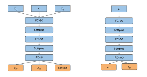
We use a latent SDE model with an MLP encoder which takes in the first three frames and outputs the mean and log-variance of the variational distribution of the initial latent state and a context vector. The decoder has a similar architecture as that for the ODE2VAE model [90] and projects the -dimensional latent state into the -dimensional observation space. The posterior drift function takes in a -dimensional context vector output by the encoder and the current state and time, whereas the prior drift only takes in the current state and time. The diffusion function is composed of multiple small neural nets, each producing a scalar for the corresponding dimension such that the posterior SDE has diagonal noise. We use the same observation likelihood as that of the ODE2VAE model [90]. We comment that the overall parameter count of our model (11605) is smaller than that of ODE2VAE for the same task (12157).
The latent ODE baseline was implemented with a similar architecture, except is does not have the diffusion and prior drift components, and its vector field defining the ODE does not take in a context vector. Therefore, the model has slightly fewer parameters (10573) than the latent SDE model. See Figure 10 for overall details of the architecture.
The main hyperparameter we tuned was the coefficient for reweighting the KL. For both the latent ODE and SDE, we considered training the model with a reweighting coefficient in , either with or without a linear KL annealing schedule that increased from to the prescribed value over the first iterations of training.
9.13 Stochastic Adjoint Implementation
We include the core implementation of the stochastic adjoint, assuming access to a callable Brownian motion bm, an Euler-Maruyama integrator ito_int_diag for diagonal noise SDEs, and several helper functions whose purposes can be inferred from their names.