The spreading of viruses by airborne aerosols: lessons from a first-passage-time problem for tracers in turbulent flows
Abstract
We study the spreading of viruses, such as SARS-CoV-2, by airborne aerosols, via a new first-passage-time problem for Lagrangian tracers that are advected by a turbulent flow: By direct numerical simulations of the three-dimensional (3D) incompressible, Navier-Stokes equation, we obtain the time at which a tracer, initially at the origin of a sphere of radius , crosses the surface of the sphere for the first time. We obtain the probability distribution function and show that it displays two qualitatively different behaviors: (a) for , has a power-law tail , with the exponent and the integral scale of the turbulent flow; (b) for , the tail of decays exponentially. We develop models that allow us to obtain these asymptotic behaviors analytically. We show how to use to develop social-distancing guidelines for the mitigation of the spreading of airborne aerosols with viruses such as SARS-CoV-2.
Keywords:
airborne aerosols; first-passage time; turbulenceI Introduction
By 1 June 2020 (14:31 GMT) the COVID-19 coronavirus pandemic had affected countries and territories and international conveyances; the numbers of cases and deaths were, respectively, and worldometer. Social distancing has played an important role in mitigation strategies that have been used in several countries to arrest the spread of COVID-19 socialdistancing. To optimise social-distancing guidelines we must ask: How far, and how fast, do small respiratory droplets or virus-bearing aerosols spread in turbulent flows? Given the ongoing COVID-19 pandemic, it is important and extremely urgent to have at least a semi-quantitative answer to this question. SARS-CoV-2, the virus that causes COVID-19, spreads, principally, in two different ways: (1) First: Respiratory droplets, ejected by the sneeze or cough of a patient, fall on nearby surfaces or persons; in this case, approximate estimates of the distance, over which droplets are likely to travel, are available NYTarticle; bourouiba2014; bourouiba2020. (2) Second: Transmission of this virus can occur because of airborne aerosols, such as, (a) a cloud of fine droplets, with diameters smaller than 5 micrometers, emitted by an infected person while speaking loudly laserlink or (b) the SARS-CoV-2 RNA on fine, suspended particulate matter Setti2020. These aerosols may remain suspended in the air for a long time. Indeed, they have been reported in two hospitals in Wuhan Liu2020; and there is growing evidence that the SARS-CoV-2 virus could also spread via airborne aerosols laserlink; Setti2020; Liu2020; Prather2020; Somsen2020, typically indoors Indoor2020. Other diseases can also spread because of airborne aerosols; examples include measles Riley1978, chickenpox Leclair1980, tuberculosis Escombe2007, and avian flu Zhao2019.
The typical sedimentation speed for such aerosols is comparable to their thermal speed. Therefore, at the simplest level, it is natural to model these aerosol particles as neutrally-buoyant Lagrangian tracers, which are advected by the flow, but are passive, in the sense that they do not affect the flow velocity. We can then study the spread of viruses, such as SARS-CoV-2, via the airborne-aerosol route, by considering the advection of such tracers by turbulent fluid flows. There have been extensive studies of such tracers in the fluid-dynamics literature Falkovich2001; Toschi2009; and models for such tracers have been used, inter alia, to model the dispersion of pheromones by lepidoptera Celani2014.
We would like to determine the time that an aerosol particle (one of the red particles in the schematic diagram of Fig. 1) takes to travel a distance from its source (the man at the centre of Fig. 1). In a turbulent flow, this time is random; furthermore, a tracer particle can go past the distance , turn back, and reach again. It is important, therefore, to calculate the time it takes for an aerosol particle to reach the distance for the first time and to calculate the probability distribution function (PDF) of the first-passage time of a tracer in a turbulent flow. We carry out this calculation below.
Specifically, we consider Lagrangian tracer particles that emanate from a point source in a turbulent fluid. If is the time at which a tracer, initially at the origin of a sphere of radius , crosses the surface of the sphere for the first time, what is the probability distribution function (PDF) )? The answer to this question is of central importance in both fundamental nonequilibrium statistical mechanics bray2013persistence; chandrasekhar1943stochastic; redner2001guide; balakrishnan2008elements; ralf2014first and in understanding the dispersal of tracers by a turbulent flow, a problem whose significance cannot be overemphasized, for it is of relevance to the advection of (a) airborne viruses, as we have noted above, and (b) pollutants in the atmosphere. First-passage-time problems have been studied extensively chandrasekhar1943stochastic; redner2001guide; balakrishnan2008elements; ralf2014first and they have found applications in a variety of areas in physics and astronomy, chemistry weiss1967first, biology ricciardi1999outline, and finance chicheportiche2014some. In the fluid-turbulence context, different groups have studied zero crossings of velocity fluctuations kailasnath1993zero or various statistical measures of two-particle dispersion, including exit-time statistics for such dispersion in two- and three-dimensional (2D and 3D) turbulent flows boffetta2002statistics; vulpiani2001exit. In contrast to these earlier studies (e.g., Refs. boffetta2002statistics; vulpiani2001exit; lalescu2018tracer), the first-passage-time problem we pose considers one tracer in a turbulent flow that is statistically homogeneous and isotropic. To the best of our knowledge, this first-passage problem has not been studied hitherto. For such a particle we show, via extensive direct numerical simulations (DNSs), that displays a crossover between two qualitatively different behaviors: (a) for , , with the integral scale of the turbulent flow and the exponent ; (b) for , has an exponentially decaying tail (Fig. 2). We develop models that allow us to obtain these two asymptotic behaviors analytically. Most important, we show how to use to obtain estimates of social-distancing guidelines for the mitigation of the spreading of airborne aerosols with viruses such as SARS-CoV-2.

II Models, Methods, and Results

The 3D incompressible, Navier-Stokes equation is
| (1a) | |||
| and | |||
| (1b) | |||
Here, is the Eulerian velocity at position at time , is the pressure field, and is the kinematic viscosity of the fluid; the constant density is chosen to be unity. Our direct numerical simulation (DNS) uses the pseudo-spectral method canuto1988spectral, with the rule for dealiasing, in a triply periodic cubical domain with collocation points; we employ the second-order, exponential, Adams-Bashforth scheme for time stepping bhatnagar2016long. We obtain a nonequilibrium, statistically stationary turbulent state via a forcing term , which imposes a constant rate of energy injection lamorgese2005direct; sahoo2011systematics, in wave-number shells and in Fourier space; this turbulent state is statistically homogeneous and isotropic.
To obtain the statistical properties of Lagrangian tracers, which are advected by this turbulent flow, we seed the flow with independent, identical, tracer particles. If the Lagrangian displacement of a tracer, which was at position at time , is , then its temporal evolution is given by
| (2) |
where is its Lagrangian velocity. In Eq. (2), we need the Eulerian flow velocity at off-grid points; we obtain this by tri-linear interpolation; and we use the first-order Euler method for time marching (see, e.g., Ref. bhatnagar2016long). We give important parameters for our DNS runs in Table 1. These include the time step , the energy dissipation rate , where is the energy spectrum, the Taylor-microscale , where the total energy , the Taylor-microscale Reynolds number , where is the root-mean-square velocity of the flow; is the integral length scale and is the integral-scale eddy-turnover time; and are, respectively, the Kolmogorov dissipation length and time scale; and is the maximum wave number that we use in our DNS.
Clearly, is the first time at which becomes equal to . Instead of computing the PDF (or histogram) of numerically, we calculate the complementary cumulative probability distribution function (CPDF) , by using the rank-order method mit+bec+pan+fri05, to circumvent binning errors. In Fig. 2, we present log-log and semi-log plots of versus , for several values of . From Fig. 2 (a) we conclude that, for , , for large , with ; note that, in this power-law scaling regime, the complementary CPDFs for different values of collapse onto a universal scaling form, if we plot . In contrast, Fig. 2 (b) shows that, for , the tail of decays exponentially. For the first-passage-time PDF, these results imply that
| (3) |
We now develop models that allow us to understand these two asymptotic behaviors analytically.
For the power-law behavior of , in the range , we construct the following, natural, ballistic model: Tracer particles emanate from the origin with (a) a velocity whose magnitude is a random variable with a PDF ; and (b) when it starts out from the origin, the tracer’s velocity vector points in a random direction. Tracers move ballistically, for short times. Therefore, for , the first-passage time ; and the first-passage PDF is
| (4) |
In statistically homogeneous and isotropic and incompressible-fluid turbulence, each component of the Eulerian velocity has a PDF that is very close to Gaussian pramanareview, so has the Maxwellian gotoh2002velocity form
| (5) |
where depends on the spatial dimension , and for , and . We substitute Eq. (5) in Eq. (4); then, by integrating over , we obtain
| (6) |
Therefore, in the limit of small and large , the first-passage-time probability is
| (7) |
this power-law exponent is the same as the one we have obtained from our DNSs above (Table 1 and Fig. 2).
We can obtain the tail for as follows. At times that are larger than the typical auto-correlation time of velocities in the Lagrangian description, we follow Taylor tay22 and assume that the motion of a tracer particle is diffusive. Therefore, we consider a Brownian particle in three dimensions (3D). To calculate the first-passage-time PDF, we must first obtain the survival probability , i.e., the probability that the particle has not reached the surface of the sphere of radius up to time , if it has started from the origin of this sphere. We start with the forward Fokker-Planck equation balakrishnan2008elements; Risken for the PDF of finding the particle at a distance from the origin at time :
| (8) |
where is the diffusion constant; this PDF satisfies the initial condition, and the absorbing boundary condition , for all at . We obtain the following solution:
| (9) |
whence we get
| (10) |
where, in the last step, we have used Eq. (9). The first-passage-time probability is
| (11) |
At large times, the first term () is the dominant one; therefore,
| (12) |
the exponential form that we have obtained from our DNS (Fig. 2 (b)); the pre-factor cannot be extracted reliably from our DNS data, because this requires much longer runs than are possible with our computational resources.
We now show that both the small- and large- behaviors of in Eq. (3) can be obtained from one stochastic model for the motion of a particle. The simplest such model uses a particle that obeys the following Ornstein-Uhlenbeck (OU) model:
| (13a) | ||||
| (13b) | ||||
Here, and are positive constants; and are the Cartesian components of the position and velocity of the particle; in three dimensions, , and ; is a zero-mean Gaussian white noise with and ; this noise is such that the fluctuations-dissipation theorem (FDT) holds. Note that there is no FDT for turbulence. However, for the one-particle statistics that we consider, the simple OU model is adequate. We use particles; for each particle, the initial-position components are distributed randomly and uniformly on the interval ; and the velocity components are chosen from a Gaussian distribution. For each particle, we obtain, numerically, the time at which it reaches a distance from the origin for the first time. We then obtain the first-passage-time complementary CPDF , which we plot in Fig. 3, for and , where , the natural length scale for Eq. (13), plays the role of in our DNSs above (Table 1 and Fig. 2). We find
| (14) |
these are the OU-model analogs of our DNS results Eq. (3). We have carried out two OU-model simulations: (a) we have designed the first, with , to explore the form of in the ballistic regime ; (b) the second, with , allows us to uncover the form of in the diffusive regime . (From a numerical perspective, it is expensive to obtain the precise form of in both ballistic and diffusive regimes, with one value of .) We now explore in detail the forms of in these two regimes. In Fig. 3(a), we present log-log plots of the complementary CPDFs of the scaled first-passage time , for and . The complementary CPDFs of , for , , and , collapse onto one curve; i.e., in this regime, scales as , which is a clear manifestation of ballistic motion. In Fig. 3(b), we present semi-log plots of the complementary CPDFs of the scaled first-passage time , for and . The complementary CPDFs of , for , , , and , collapse onto one curve; from this we conclude that, in this regime, scales as , which is a clear signature of diffusive motion.

III Conclusions and Discussion
We have defined and studied a new first-passage-time problem for Lagrangian tracers that are advected by a 3D turbulent flow that is statistically steady, homogeneous and isotropic. Our work shows that the first-passage-time PDF has tails that cross over from a power-law form to an exponentially decaying form as we move from the regime to (Eq. (3)). We develop ballistic-transport and diffusive models, for which we can obtain these limiting asymptotic behaviors of analytically. We also demonstrate that an OU model, with Gaussian white noise, which mimics the effects of turbulence, suffices to obtain the crossover between these limiting forms. Of course, such a simple stochastic model cannot be used for more complicated multifractal properties of turbulent flows vulpiani2001exit; pramanareview; arneodo.
Earlier studies have concentrated on two-particle relative dispersion by using doubling-time statistics, in 2D fluid turbulence; in particular, they have shown that the PDF of this doubling time has an exponential tail boffetta2002statistics. Studies of velocity zero crossings kailasnath1993zero, in a turbulent boundary layer, have shown that PDFs of the zero-crossing times have exponential tails.
The single-particle first-passage-time statistics that we study have not been explored so far. Furthermore, can be used to to develop social-distancing guidelines for the mitigation of the spreading of airborne aerosols with viruses such as SARS-CoV-2 as we show below.
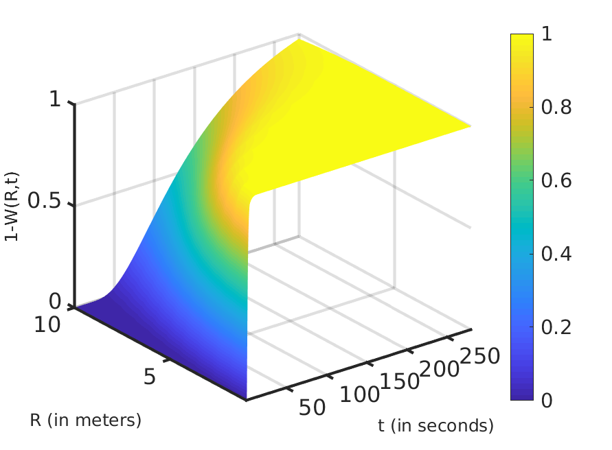
Given a pseudospectral DNS, of the type we have carried out, we can obtain the integral scale and from the energy spectrum , as we have noted above. A recent study of COVID-19 in municipalities in China suggests that a very large fraction of COVID-19 infections occur because of indoor transmission of the SARS-CoV-2 virus Indoor2020. Therefore, it is important to study such transmission in rooms and offices; a comprehensive DNS study of the Navier-Stokes equation, with the correct boundary conditions enforced at every wall and surface in the room and accurate forcing functions (dictated, e.g., by fans and vents), is a considerable challenge. Furthermore, it is not possible to carry out such a DNS for every room with a different arrangement of the furniture in it. Hence, it is important to come up with semi-quantitative criteria that help us to understand, and mitigate, the indoor transmission of such virues. Turbulence models have been used to study the flow of air in rooms and offices li2005multi; zhang2007evaluation; from these models and related experiments we obtain the estimate m/s in a typical office. We must also estimate , for it is an important crossover length scale in our analysis of . In our DNS is , where is the linear size of our simulation domain. In a typical office or a train, with fixed forcing, via fans or vents, we use to be approximately a few meters; of course, must depend on the degree of crowding on a train or the number of cubicles in a large office room. Now consider one infected person who is at a distance from another person. The probability of virus-laden aerosol particles not reaching the second person, up until time is related to as follows:
| (15) |
which we calculate, by using Eq. (11), and depict in Fig. 4(a) and Fig. 4(b), in the diffusive regime; Fig. 4(a) is a surface plot of versus and , for the representative values m and m/s; Fig. 4(b) gives a surface plot of versus the dimensionless parameters and , where . (We give similar plots for the ballistic regime in the Supplemental Material.) In Table 2 we give the values of for different values of and . These figures and Table 2 lead to three clear observations:
- 1.
If the separation , i.e., we have to consider the ballistic regime (see the Supplementary Material), then goes very rapidly to (i.e., the aerosol particle reaches the second person), even if is very small.
- 2.
The smaller the separation , between two persons, the shorter the time in which becomes very small, i.e., the aerosol particles reach from one person to the other.
- 3.
Our calculation leads to quantitative predictions; e.g., if the separation , i.e., we have to consider the diffusive regime, then goes to in tens of seconds, if m, and in hundreds of seconds, m, for the representative parameters that we use to obtain Table 2. A recent study vancovid has suggested that the SARS-CoV-2 virus remains viable in aerosols for nearly hours. Therefore, if the concentration of virus-laden aerosols is high in a poorly ventilated room, then we must employ more stringent social-distancing norms than are in place now, even if people spend only tens of minutes together in such a room.
| s | s | s | s | s | s | s | s | |
|---|---|---|---|---|---|---|---|---|
| m | ||||||||
| m | ||||||||
| m | ||||||||
| m | ||||||||
| m | ||||||||
| m | ||||||||
| m | ||||||||
| m | ||||||||
| m |

The methods that we have developed can be applied, mutatis mutandis, (a) in sophisticated models for virus particles or droplets, e.g., those that use inertial particles Cencini2006; Salazar2009 or multi-phase flows Balachandar2010; Pal2016 and (b) in turbulent flows that are not statistically homogeneous and isotropic. We will examine these in future work. At the moment, it is important to use our minimal model to obtain semi-quantitative for social-distancing guidelines, as we have done above.
Acknowledgements.
D.M. and A.B. thank John Wettlaufer for useful discussions. A.K.V. and R.P. thank Jaya Kumar Alageshan for discussions and for help with Fig. 1, and CSIR (IN) and DST (IN) for financial support. A.B. and D.M. are supported by the grant Bottlenecks for Particle Growth in Turbulent Aerosols from the Knut and Alice Wallenberg Foundation (Dnr. KAW 2014.0048); the computations were performed on resources provided by the Swedish National Infrastructure for Computing (SNIC) at PDC and SERC (at IISc).References
- (1) These data are updated in real time at https://www.worldometers.info/coronavirus/ .
- (2) See, e.g., https://www.cdc.gov/coronavirus/2019-ncov/prevent-getting-sick/social-distancing.html .
- (3) https://www.nytimes.com/interactive/2020/04/14/science/coronavirus-transmission-cough-6-feet-ar-ul.html?campaign_id=57&emc=edit_ne_20200414&instance_id=17644&nl=evening-briefing®i_id=75908386&segment_id=25175&te=1&user_id=fb4f001a71c3b41abab178e84896d909 and reference therein.
- (4) Bourouiba, L., Dehandschoewercker, E., and Bush, J.W.M., Violent respiratory events: on coughing and sneezing, J. Fluid. Mech. 745, 537-563, (2014)
- (5) Bourouiba, L., Turbulent Gas Clouds and Respiratory Pathogen Emissions Potential Implications for Reducing Transmission of COVID-19, Journal of the American Medical Association (JAMA); published online March 26, 2020. doi:10.1001/jama.2020.4756.
- (6) https://www.electrooptics.com/news/laserimaging-tech-shows-how-covid-19-spread-talking .
- (7) Setti, L., Passarini, F., De Gennaro,i G., Baribieri, P., Perrone, M.G., Borelli, M., Palmisani, J., Di Gilio, A., Torboli, V., Pallavicini, A., et al., SARS-Cov-2 RNA Found on Particulate Matter of Bergamo in Northern Italy: First Preliminary Evidence:https://www.medrxiv.org/content/10.1101/2020.04.15.20065995v1 (article submitted for peer-review publication).
- (8) Liu, Y., Ning, Z., Chen, Y., et al., Aerodynamic analysis of SARS-CoV- in two Wuhan hospitals, Nature (2020)
- (9) Prather, K.A., Wang, C.C., and Schooley R.T., Reducing transmission of SARS-CoV-2, Science 10.1126/science.abc6197 (2020).
- (10) Somsen, G.A., van Rijn, C., Kooij, S., Bem, R.A., Bonn, D., Small droplet aerosols in poorly ventilated spaces and SARS-CoV-2 transmission, Lancet Respir Med 2020; Published Online May 27, 2020 https://doi.org/10.1016/S2213-2600(20)30245-9 .
- (11) Hua, Q., Te, M., Li, L., Xiaohong, Z., Danting, L., and Yuguo, L, Indoor transmission of SARS-CoV-2 , medRxiv preprint doi: https://doi.org/10.1101/2020.04.04.20053058 ; this version posted April 7, 2020.
- (12) Riley, E.C., Murphy, G., Riley, R.L., Airborne spread of measles in a suburban elementary school, Am J Epidemiol. 1978 May;107(5):421-32. PMID: 665658 DOI: 10.1093/oxfordjournals.aje.a112560.
- (13) Leclair, J.M., Zaia, J.A., Levin, M.J., Congdon, R.G., and Goldmann, D.A., Airborne transmission of chickenpox in a hospital, N. Engl. J. Med. 302, 450–453 (1980). https://doi.org/10.1056/NEJM198002213020807.
- (14) Escombe, A.R., et al., The detection of airborne transmission of tuberculosis from HIV-infected patients, using an in vivo air sampling model, Clin. Infect. Dis. 44, 1349–1357 (2007). https://doi.org/10.1086/515397.
- (15) Zhao, Y., Richardson, B., Takle, E., Cahi, L., Schmitt, D., and Xin, H., Airborne transmission may have played a role in the spread of 2015 highly pathogenic avian influenza outbreaks in the United States, Scientific Reports, (2019) 9:11755; https://doi.org/10.1038/s41598-019-47788-z .
- (16) Falkovich, G., Gawȩdzki, K., and Vergassola, M., Particles and fields in fluid turbulence, Rev. Mod. Phys. 73, 913 (2001).
- (17) Toschi, F., and Bodenschatz, E., Lagrangian properties of particles in turbulence, Annu. Rev. Fluid Mech. 41, 375 (2009).
- (18) Celani, A., Villermaux, E., and Vergassola, M., Odor Landscapes in Turbulent Environments, Phys. Rev. X 4, 041015 (2014).
- (19) Bray, A.J., Majumdar, S., and Scher, G., Adv. Phys. 62, 3, (2013).
- (20) Chandrasekhar, S., Rev. Mod. Phys. 15, 1 (1943).
- (21) Redner, S., A guide to first-passage processes (Cambridge University Press, 2001).
- (22) Balakrishnan, V., Elements of Nonequilibrium Statistical Mechanics (Ane Books, 2008).
- (23) Ralf, M., Sidney, R., and Gleb, O., First-passage phenomena and their applications (World Scientific, 2014).
- (24) Weiss, G.H., Adv. Chem. Phys. 13, 1 (1967).
- (25) Ricciardi, L., Crescenzo, A., Giorno, V., and Nobile, A., Math. Japonica 50, 247 (1999).
- (26) Chicheportiche, R., and Bouchaud, J.-P. First-Passage Phenomena and Their Applications (World Scientific, 2014).
- (27) Kailasnath, P. and Sreenivasan, K., Phys. Fluids A 5, 2879 (1993).
- (28) Boffetta, G. and Sokolov, I.M., Phys. Fluids 14, 3224 (2002).
- (29) Vulpiani, A., et al., Intermittency in Turbulent Flows, eds. J. C. Vassilicos, (Cambridage University Press 2001), 223.
- (30) Lalescu, C.C. and Wilczek, M., New J. Phys. 20, 013001 (2018).
- (31) Canuto, C., Hussaini, M., Quarteroni, A., and Zang, T., Spectral methods in fluid dynamics Springer, Berlin, 1988.
- (32) Bhatnagar, A., Gupta, A., Mitra, D., Pandit, R., and Perlekar, P., Phys. Rev. E 94, 053119, (2016).
- (33) Lamorgese, A., Caughey, D., and Pope, S., Phys. Fluids 17, 015106 (2005).
- (34) Sahoo, G., Perlekar, P., and Pandit, R., New J. Phys. 13, 013036 (2011).
- (35) Mitra, D., Bec, J., Pandit, R., and Frisch, U., Phys. Rev. Lett 94, 194501 (2005).
- (36) Pandit, R., Perlekar, P., and Ray, S.S., Pramana 73, 179 (2009).
- (37) Gotoh, T., Fukayama, D., and Nakano, T., Phys. Fluids 14, 1065 (2002).
- (38) Taylor, G.I., Proc. London. Math. Soc. 20, 196 (1922).
- (39) Risken, H.Z., The Fokker-Planck Equation (Springer, Berlin, 1989).
- (40) Arneodo, A., Benzi, R., Berg, J., Biferale, L., Bodenschatz, E., Busse, A., et al., Phys. Rev. Lett. 100, 254504, (2008).
- (41) Li, Y., S. Duan, I.T. Yu, and T.W. Wong, Multi-zone modeling of probable SARS virus transmission by airflow between flats in Block E, Amoy Gardens, Indoor Air 15:96-111 (2005).
- (42) Zhang, Z., Zhang, W., Zhai, Z.J., and Chen, Q.Y., HVAC R Research, 13, 6:871–86, (2007).
- (43) Cencini, M., Bec, J., Biferale, L., Boffetta, G., Celani, A., Lanotte, A., Musacchio, S., and Toschi, F., Dynamics and statistics of heavy particles in turbulent flows, J. Turbul. 7, N36 (2006).
- (44) Salazar, J.P.L.C. and Collins, L.R., Two-particle dispersion in isotropic turbulent flows, Annu. Rev. Fluid Mech. 41, 405 (2009).
- (45) Balachandar, S. and Eaton, J.K., Turbulent dispersed multiphase flow, Annu. Rev. Fluid Mech. 42, 111–133 (2010).
- (46) Pal, N., Perlekar, P., Gupta, A., and Pandit, R., Binary-fluid turbulence: Signatures of multifractal droplet dynamics and dissipation reduction, Phys. Rev. E 93, 063115 (2016).
- (47) van Doremalen, N., Bushmaker, T., Morris, D.H., et al. Aerosol and Sur face Stab ility of SARS-CoV-2 as Compared with SARS-CoV-1. N Engl J Med (2020) published online March 17. https://www.nejm.org/doi/full/10.1056/NEJMc2004973?query=featured_home
Supplemental Materials:The spreading of viruses by airborne aerosols: lessons from a first-passage-time problem for tracers in turbulent flows Akhilesh Kumar Verma Akshay Bhatnagar Dhrubaditya Mitra Rahul Pandit
In this Supplemental Material, we provide the following:
(a) Consider one infected person, who is at a distance from another person. We give surface plots of the probability of a virus-laden aerosol particle not reaching the second person, up until time , in the ballistic regime (Fig. S1). We also give surface plots of , the probability that a virus-laden aerosol particle reaches the second person, at time , for the first time for ballistic (Fig. S2) and diffusive (Fig. S3) cases.
(b) The energy spectrum from our direct numerical simulation of the three-dimensional Navier-Stokes equation (see the main paper). A log-log plot of this spectrum (red curve) is given in Fig. S4; for comparison, we show the Kolmogorov scaling form (black line).