Throughput Maximization of Mixed FSO/RF UAV-aided Mobile Relaying with a Buffer

In beyond fifth-generation (B5G) with a presence of ultra-dense heterogeneous small cells, wireless backhaul/fronthaul networks requires to comply with ultra-high network throughput. In this regard, several industry project [9] and academe [10, 11, 12, 13] have paid attention to this challenge and researched a free space optical communication (FSO) on the mobile relaying system as a promising solution. Particularly, by taking some advantage of FSO (e.g., unlicensed broad spectrum, immunity to electromagnetic interference, and security), Facebook had launched project Aquila which employs FSO communication for the source to UAV-assisted relay link and UAV-to-UAV link, to support the high throughput in the air-to-ground (A2G) and air-to-air channel. Motivated by the potential of FSO-assisted mobile relaying, our previous works of [12, 13] investigated the point-to-point (PtP) FSO link for UAV-to-ground user terminal (i.e., single-hop communication).

Besides, extensive works in academia have developed to exploit the benefits of FSO-based communication and also have accordingly adopted a mixed FSO/RF system to utilize both RF and FSO links. Particularly, to consider the dual-hop system (e.g., relaying system), the mixed FSO/RF communication has been investigated [14, 15, 16, 17]. In [14], the dual-hop mixed FSO/RF backhauling scenario using networked flying platforms (NFPs) has been proposed. The efficacy of the network scenario has been shown in terms of link budget and achievable data rate for only the single FSO link under different weather conditions. Furthermore, in [15, 16], the performance analysis of mixed FSO/RF systems following the general turbulent fading model has been provided. As identified in these works, the attenuation condition is a major challenge in dual-hop mixed FSO/RF communication, especially for A2G link. In addition, the rate imbalance problem, which caused by using other types of links, is another major concern.

To address the practical issues in the asymmetric dual-hop relay system (e.g., dual-hop relay transmission with mixed FSO/RF link), the conventional works [17, 18, 19] have focused on the buffer-assisted relaying. Note that it is practical to consider the buffering in relaying, since the actual relay system includes a buffer. In particular, [17] demonstrated that buffering can enhance system performance under various mixed FSO/RF link conditions. In addition, the authors in [19] suggested the design of FSO-based buffer-aided cooperative protocols and showed that the buffering on FSO-assisted relay constitutes an additional DoF at the expense of increased delay. Not only just buffer-related conditions, but also average delay in the buffer-aided relaying system, have been addressed [20, 21, 22, 23]. In [20], the two buffer-aided relaying protocols are proposed, and the throughput-delay tradeoff and average delay for the buffer-aided relaying system are further analyzed. Moreover, to consider the practical delay-constrained application, [21] studied two transmission schemes for buffer-aided relaying; delay-limited transmission (e.g., real-time) and delay-tolerant transmission. Delay-limited traffic, for example, supports delay-sensitive services which include voice over internet protocol, video conferencing, and monitoring of critical processes (e.g., medical packet) [24]. On the other hand, delay-tolerant traffic does not carry an urgency and can be served when the reliable reception is essential, e.g., email, instant messages, or sensor data in periodic sensing [25]. For both delay-limited and delay-tolerant transmission, authors in [21] analyzed a hybrid FSO/RF backhauling policy to satisfy a certain delay requirements.

By taking into consideration the aforementioned features, e.g., mobility, buffering, and delay consideration in relaying system, we focus on the scenario of dual-hop mixed FSO/RF backhauling with the help of buffer, which can be a promising solution to the emerging wireless backbone network as discussed in [14, 13, 12]. In such a scenario, we study on the end-to-end optimization of a mixed FSO/RF-based mobile relaying system. In order to deal with the transmission rate imbalance between FSO and RF links¹¹ 1 Since FSO communication utilizes license-free narrow beams with a wide frequency spectrum (more bandwidth can be provided for FSO link than RF link, i.e., $B_{\mathrm{FSO}}\geq B_{\mathrm{RF}}$), it can offer data rates higher than the baseline alternatives (e.g., RF communication). according to the relay’s location, we further regard both buffer and average delay constraints on the UAV relay node. We have summarized the main contributions of this work as follows:

• •

  Unlike [14, 12], which have investigated the only single hop scenario in mixed FSO/RF backhaul links, we deeply look into the scenario depicted in Fig. 1, in which dual-hop mixed FSO/RF backhauling is operated on the UAV-assisted relaying under a limited buffer constraint. Especially, we solve the trajectory optimization for the throughput maximization in this system. To the best of our knowledge, there is no open literature to tackle the optimization of the buffer-constrained mobile relaying system in dual-hop mixed FSO/RF links.

• •

  Furthermore, we consider buffer constraints to account for practical relaying scenarios and the transmission rate imbalance in a mixed FSO/RF system, which is induced by using a different type of links (i.e., FSO link for source-to-relay and RF link for relay-to-destination). In other words, the UAV relay node is equipped with a buffer of finite queue size and can control throughput delay and UAV mobility.

• •

  Moreover, we design the system by classifying two relay transmission schemes (i.e., i) delay-tolerant transmission and ii) delay-limited transmission) according to the average delay requirements of the network data throughput. Specifically, we design the system where the data should be transmitted at the relay node below the average delay.

• •

  To tackle these non-convex trajectory optimization problems, we propose an iterative algorithm by utilizing the successive optimization method to find the locally optimal solution. Then, the trajectories can be established by applying quadratically constrained programming (QCP).

• •

  Under different conditions, e.g., visibility, buffer size, and delay limit, the simulation results for throughput maximized trajectories are drawn. Based on the buffer and delay constraints, the throughput-delay and the throughput-buffer tradeoff are presented. Consequently, we validate the supremacy of the proposed scheme compared to conventional schemes (e.g., static relaying [3] and data-ferrying relaying [26, 5]) according to the simulation and numerical results.

The remainder of this paper is organized as follows: In Section II, the system model for the FSO and RF links and the metrics for the buffer constraint of dual-hop mixed FSO/RF network are presented. The throughput maximization problem for buffer-aided mobile relaying is formulated and optimized by two delay-considered transmission schemes (e.g., delay-limited transmission and delay-tolerant transmission) in Section III. In Section IV, numerical results are presented, and concluding remarks are drawn in Section V.

Notation: Throughout this paper, we use the normal-face font to denote scalars, and boldface font to denote vectors. We use $\mathbb{R}^{D\times 1}$ to represent the $D$-dimensional space of real-valued vectors. We also use $\|\cdot\|$ to denote the $L^{2}$-norm (i.e., an Euclidean norm) and $\mathrm{log}(\cdot)$ to represent a natural logarithm. The expression $O(\cdot)$ stands for describing the Big O notation.

For an FSO link, the channel gain at a link distance $l_{\mathrm{FSO}}$, based on the Beer-Lambert Law³³ 3 Note that, if other attenuation factors, e.g., rain, snow, and haze, need to be considered, the optimization framework can be solved by adjusting only some parameters, e.g., $\beta$ or $k_{2}$., can be expressed as

where $\beta_{\mathrm{dB}}=\frac{3.91}{V}\left(\frac{\lambda_{0}}{550\ \mathrm{[nm]}}\right)^{-p}\ \mathrm{[dB/km]}$ depends on the wavelength $\lambda_{0}$ assumed to be 1550 [nm] as an example in this paper, $V$ is the visibility in [km], and the size distribution coefficient $p$ is determined by Kim model [28]. Note that $\beta=\frac{\beta_{\mathrm{dB}}\cdot\log{10}}{10^{4}}\ \mathrm{[m^{-1}]}$.

While the capacity of the FSO channel has not been known in a closed-form, the capacity bounds of FSO have been proposed in several papers. To describe the data rate of an FSO link between source and relay, we use the lower bound of FSO capacity in intensity channel introduced in [29]. The average electrical SNR (ASNR) is given by $\gamma_{\mathrm{FSO}}^{2}=\frac{\varepsilon^{2}}{\sigma_{\mathrm{FSO}}^{2}}$, where $\varepsilon$ and $\sigma_{\mathrm{FSO}}^{2}$ are the average optical power and noise variance for FSO, respectively. The parameter, $k_{1}$, related to ASNR and parameter, $k_{2}$, related to attenuation condition are formulated, respectively, as

Note that $\mu$ is the free parameter that indicates the solution to the equation $\alpha_{0}=\frac{1}{\mu^{*}}-\frac{e^{-\mu^{*}}}{(1-e^{-\mu^{*}})}$ in which the average-to-peak ratio (APR) is set to $\alpha_{0}=\frac{\varepsilon}{\lambda_{0}}$ where $\lambda_{0}$ is the peak optical power.

The FSO link achievable rate for the time slot $n$ in bits/second (bps) is given by the channel gain for FSO link in (1), the $k_{1}$ and $k_{2}$ in (2) and (3), the bandwidth in hertz (Hz) for FSO link $B_{\mathrm{FSO}}$, and the received ASNR $\bar{\gamma}_{\mathrm{FSO}}^{2}=h_{\mathrm{FSO}}^{2}\cdot\gamma_{\mathrm{FSO}}^{2}$ as follows:

Note that we assume that precise pointing, acquisition, and tracking (PAT) algorithm may compensate for the pointing error.

For an RF link between the UAV-aided relay and the user terminal, the channel gain $h_{\mathrm{RF}}$ can be expressed as

where $\tau_{\mathrm{RF}}[n]$ and $\tilde{h}_{\mathrm{RF}}[n]$ account for the effect of large-scale fading (e.g., path loss and shadowing) and the effect of small-scale fading with $\mathbb{E}\{|\tilde{h}_{\mathrm{RF}}[n]|^{2}\}=1$, respectively. Furthermore, for UAV-ground RF link, the large-scale attenuation is usually modeled with the probabilities of LoS and non-LoS (NLoS) links⁴⁴ 4 Note that, due to the shadowing effect and the reflection of signals from obstacles, different large-scale attenuation models need to be considered for LoS and NLoS links. . As in [30], $\tau_{\mathrm{RF}}[n]$ is expressed as

where $\beta_{0}$ represents the received power at the reference distance $d_{0}=1$ [m], $l_{\mathrm{RF}}$ denotes a link distance between $\mathcal{R}$ and $\mathcal{D}$, $\tilde{\alpha}$ is the path loss exponent⁵⁵ 5 $\tilde{\alpha}$ represents the more general path loss exponent $\tilde{\alpha}\geq 2$, rather than the special case of $\tilde{\alpha}=2$ which only considers free-space condition., and $\kappa$ is an additional attenuation factor due to the NLoS link. As a result, $h_{\mathrm{RF}}[n]$ is a random variable with the random occurrence of LoS and NLoS as well as the random small-scale fading. Accordingly, the expected channel gain by averaging over both randomness is given by [31],

where $\hat{P}_{\mathrm{LoS}}[n]=P_{\mathrm{LoS}}[n]+(1-P_{\mathrm{LoS}}[n])\kappa$, and $P_{\mathrm{LoS}}[n]=\frac{1}{1+C\cdot\mathrm{exp}(-D[\theta[n]-C])}$ is the LoS probability between UAV and the user terminal in which $C$ and $D$ are the parameters depending on the propagation condition, and $\theta[n]=\frac{180}{\pi}\mathrm{sin}^{-1}(\nicefrac{{H}}{{l_{\mathrm{RF}}[n]}})$ is the elevation angle in degree.

The achievable rate in bps between UAV and the user terminal with the constant transmission power $P$ at time slot $n$ is expressed as

where $B_{\mathrm{RF}}$ represents the RF bandwidth in Hz, and $\sigma_{\mathrm{RF}}^{2}$ is the noise variance for RF. Note that, as the channel gain $h_{\mathrm{RF}}[n]$ is the random variable, $\hat{R}_{\mathrm{RF}}[n]$ is also a random variable. Using the concavity of (8) and Jensen’s inequality, we have

where $\tilde{\gamma}_{0}\triangleq\frac{\beta_{0}\cdot P}{\sigma_{\mathrm{RF}}^{2}}$ and $\alpha\triangleq\tilde{\alpha}/2$. It is found that () depends on the UAV location $\mathbf{q}_{\mathcal{R}}[n]$ not only over $l_{\mathrm{RF}}[n]$, but also over $\hat{P}_{\mathrm{LoS}}[n]$. For this reason, it is challenging to handle () directly. To resolve this issue, we use the homogeneous approximation of the LoS probability, i.e., $\hat{P}_{\mathrm{LoS}}[n]\simeq\bar{P}_{\mathrm{LoS}},\forall n$, as in [31]. Note that $\bar{P}_{\mathrm{LoS}}$ could be the value corresponding to the most likely elevation angle or the average value based on a certain heuristic UAV trajectory. Accordingly, () can be rewritten as $\bar{R}_{\mathrm{RF}}=\displaystyle\sum_{n=1}^{N}\frac{B_{\mathrm{RF}}}{N\log 2}\cdot\log\left(1+\dfrac{\gamma_{0}}{(\|\mathbf{q}_{\mathcal{D}}-\mathbf{q}_{\mathcal{R}}[n]\|^{2})^{\alpha}}\right)$ where $\gamma_{0}\triangleq\tilde{\gamma}_{0}\bar{P}_{\mathrm{LoS}}$. Thus, the achievable rate of RF link for the time slot $n$ is expressed as [32, 31]

It is worth noting that $\bar{R}_{\mathrm{RF}}$ is the approximation of $\mathbb{E}\{\hat{R}_{\mathrm{RF}}[n]\}$, and $R_{\mathrm{RF}}[n]$ is the corresponding average rate expression between $\mathcal{R}$ and $\mathcal{D}$ at any time slot $n$.

As shown in Fig. 2, we consider a dual-hop mixed FSO/RF network communicating between a source $\mathcal{S}$ and a destination $\mathcal{D}$ via a single UAV-enabled mobile relay node $\mathcal{R}$. Throughout the system, it is assumed that the source transmits the message in packets via an FSO link at the rate of $\mathit{C}_{\mathcal{SR}}[n]$. For ease of exposition, an amount of data rate instead of a packet rate is considered. Note that analysis based on the packet rate can also be performed by dividing the bit rate with the number of bits per packet, if necessary. For the scheduling policy at queuing node, we consider first-in-first-out (FIFO), which implies that packets are en-queued in turn, and the packets which wait longest in a buffer are de-queued first. Thanks to the independent operation of the mixed FSO/RF transmission in parallel [19], we leverage a full-duplex relaying (FDR), which works in the decode-and-forward (DF) protocol in this system. Note that the error-free condition in transmission, relaying, and detection is assumed for explaining the transmission rate, in which we deal with the buffer-aided mobile relaying based on the optimization perspective instead of the performance analysis perspective. In the following, we discuss the queuing dynamics in which source and relay transmit data as in [33, 34].

The throughput maximization problem for this transmission scheme should consider a delay in a queue; hence, we use the average delay $L$ in (17) for the delay requirement.

Since the average throughput $\Phi$ can be expressed equivalently with a sum of throughput received by the destination, we set the objective function with $\sum_{n=2}^{N}\mathit{C}_{\mathcal{RD}}[n]$. Note that we adopt the following notations to better understand the continuous variables in the optimization problems: the position of UAV $\mathcal{Q}=\{\mathbf{q}_{\mathcal{R}}[n],\ \forall n\}$, the velocity of UAV $\mathcal{V}=\{\mathbf{v}_{\mathcal{R}}[n],\ \forall n\}$, and the acceleration of UAV $\mathcal{A}=\{\mathbf{a}_{\mathcal{R}}[n],\ \forall n\}$. Thus, we formulate the throughput maximization for delay-limited transmission as the following (P1):

The constraint in (20) describes the discrete time model of UAV’s position and velocity related to the position $\mathbf{q}_{\mathcal{R}}[n]$, the velocity $\mathbf{v}_{\mathcal{R}}[n]$, as well as the acceleration $\mathbf{a}_{\mathcal{R}}[n]$. Moreover, considering practical constraints of UAV’s flight, UAV is constrained with the maximum acceleration in (21), and the maximum velocity in (22). In addition, we establish (24) to hold the buffer constraint, which limits the queue length to $L_{\mathrm{Q}}$. Note that (24) satisfies the information-causality by $\mathit{Q}[n]\geq 0$⁷⁷ 7 $\mathcal{R}$ can only forward the information which has already been received from $\mathcal{S}$, at each slot $n$. . Furthermore, delay-considered transmission yields the average delay constraint of (25), which includes the requirement value of the average delay $L^{\mathrm{req}}$. Depending on a certain delay-requirement, the delay-time limit can be flexibly managed by adjusting $L^{\mathrm{req}}$.

We note that, in some applications (e.g., sensing and border surveillance), UAV should be constrained with pre-determined initial and final positions/velocities. If necessary, the initial and final position/velocity constraints can be further considered in this framework (P1) as follows

In (26) and (27), we denote $\mathbf{q}_{\mathrm{I}}$, $\mathbf{q}_{\mathrm{F}}$, $\mathbf{v}_{\mathrm{I}}$, and $\mathbf{v}_{\mathrm{F}}$ as the initial/final positions and velocities, respectively. In this system, we do not consider these constraints to solely focus on the mobile relaying system, especially for mixed FSO/RF-enabled backhaul networks.

Despite of the convex constraints (20)-(22), the non-concave objective function $\mathit{C}_{\mathcal{RD}}[n]$ and non-convex constraints (24)-(25) cause (P1) to be a non-convex optimization problem, which therefore is quite challenging to solve with the standard convex optimization method. To address such a challenge, we first use the first-order Taylor approximation to $R_{\mathrm{RF}}[n]$ with any given local value $\mathbf{q}^{k}_{\mathcal{R}}[n]$ at the iteration $k$. Then, we lower-bound the throughput of RF as

Note that, as in [39], $\mathcal{A}^{k}$ and $\mathcal{B}^{k}$ are expressed as

Secondly, the lower bounded throughput of FSO is given by high-SNR approximation⁸⁸ 8 Since $k_{1}\cdot e^{-k_{2}\cdot\|\mathbf{q}_{\mathcal{R}}[n]-\mathbf{q}_{\mathcal{S}}\|}\gg 1$ even under the worst atmospheric conditions (e.g., heavy-fog condition), the high-SNR approximation can be applied to the achievable rate of FSO link. as

Note that $R^{k}_{\mathrm{RF}}[n]$ and $R^{k}_{\mathrm{FSO}}[n]$ are concave functions with respect to $\mathbf{q}_{\mathcal{R}}[n]$.

Now, we introduce slack variables $\mathcal{T_{S}}=\{t_{\mathcal{S}}[n]=\mathit{C}_{\mathcal{SR}}[n],\ n=1,\cdots,N\}$, $\mathcal{T_{D}}=\{t_{\mathcal{D}}[n]=\mathit{C}_{\mathcal{RD}}[n],\ n=2,\cdots,N\}$ for the non-concave objective function and replace the non-convex constraints (24)-(25) to convex constraints with $\{t_{\mathcal{S}}[n]\}_{n=1}^{N}$ and $\{t_{\mathcal{D}}[n]\}_{n=2}^{N}$. Hence, we can reformulate (P1) into the following optimization problem for any given local value $\{\mathbf{q}^{k}_{\mathcal{R}}[n]\}_{n=1}^{N}$ at the $k$-th iteration as following

where we note that, plugging (24) into (13), we can recursively rewrite the queue state as

in which $\mathit{Q}^{{}^{\prime}}[1]=t_{\mathcal{S}}[1]$. We also point out that the average delay is rewritten as $L^{{}^{\prime}}=\frac{\sum_{n=1}^{N}\mathit{Q}^{{}^{\prime}}[n]}{\sum_{n=1}^{N}t_{\mathcal{S}}[n]}$ yielding the constraint in (40).

$(\mathrm{P1}^{\star})$ is the type of convex quadratically constrained program (QCP). The convex QCP can be tackled within a polynomial complexity, by interior-point methods with a standard convex optimization solver (e.g., CVX). Therefore, we suboptimally solve (P1) via the successive convex approximation (SCA) method to (P1^⋆) by iteratively updating the local values $\{\mathbf{q}^{k}_{\mathcal{R}}[n]\}_{n=1}^{N}$ [40]. It has been proved that the SCA method converges to at least a locally optimal point [5]. We further show the convergence through the numerical results in Section IV.

In closing this subsection, we summarize the proposed successive optimization steps for the delay-limited transmission (P1) in Algorithm 1.

Previously, we have dealt with the delay-limited transmission scheme, and have studied throughput optimization on UAV-assisted mobile relaying under a limited buffer constraint. Clearly, most applications focus on the throughput and delay, which have a trade-off between them (see, e.g., [33, 35]). In contrast, some applications, such as periodic sensing, do not concern the delay as sensitively as the delay-limited application does. Hence, we address the delay-tolerant transmission scheme as a case study of (P1).

For delay-tolerant transmission scheme, the relay is allowed to store the received data in its buffer and forward it to the destination without any limit of delay. Accordingly, we can assume that the delay requirement is very loose, e.g., $L^{\mathrm{req}}$ is very large in the delay-tolerant transmission. Then, we can omit (25) since it does not affect the throughput optimization. In particular, we deal with the delay-tolerant transmission scheme by simply changing the constraint in $(\mathrm{P1}^{\star})$ as follows:

Like the problem $(\mathrm{P1}^{\star})$, the problem $(\mathrm{P2}^{\star})$ in (45) is also QCP. Then, we suboptimally solve (P2^⋆) via the successive convex optimization by iteratively updating the local points $\{\mathbf{q}^{k}_{\mathcal{R}}[n]\}_{n=1}^{N}$, which ensure to converge. Note that we can also apply Algorithm 1 to the throughput maximization of delay-tolerant transmission by replacing $(\mathrm{P1}^{\star})$ to $(\mathrm{P2}^{\star})$ and (40) to (45).

We here provide the complexity of our algorithm. In order to determine the complexity of Algorithm 1, we need to decide the complexity of subproblem (P1^⋆) described in Section III-A.

According to the complexity analysis in [41, 42], to solve the convex optimization problem especially with the interior-point methods, (ignoring any structure in the problem, such as sparsity) each step requires on the order of

operations. Note that $\zeta$ and $\xi$ denote the number of variables and constraints, respectively, and $F$ denotes the cost of evaluating the first and second derivatives of the objective and constraint functions.

For (P1^⋆), it can be easily found that $\zeta=8N+1$. Also, we can compute the number of constraints $\xi$, according to Table I at the top of next page, as $\xi=11N+4$. Therefore, comparing the order of $\zeta^{3}$, $\zeta^{2}\xi$, and $F$, it can be found that $\zeta^{2}\xi$ is greater than $\zeta^{3}$ and $F$. Note that $F$ follows $O(N)$ in the problems, whereas, $\zeta^{3}$ and $\zeta^{2}\xi$ follow $O(N^{3})$.

As a result, considering the interior point method, the computational complexity for Algorithm 1 is derived as

Note that $\vartheta$ denotes the number of iterations for steps 3 - 5 in Algorithm 1. Then, the complexity of Algorithm 1 can be reduced to the order of $O(\vartheta N^{3})$.

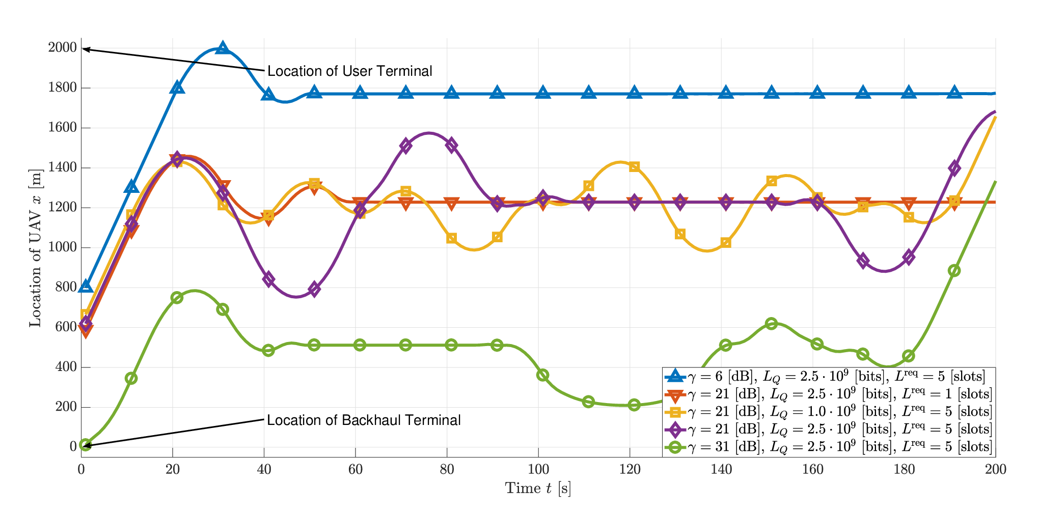
Considering the average delay requirement $L^{\mathrm{req}}$, we present the simulation results of the throughput maximization problem for delay-limited transmission (P1). In Fig. 3, the optimized trajectories in $x$-coordinate⁹⁹ 9 The backhaul terminal and user terminal are positioned horizontally on the $x$-axis. Intuitively, we can see that flying between backhaul and user terminals only on the $x$-axis is optimal, i.e., any UAV movement on the y-axis is not beneficial. Thus, we provide only the result of the $x$-axis, not the trajectory of $xy$-axis or $xyz$-axis. for the mobile relay are drawn over the different reference received SNR $\gamma$, buffer size $L_{Q}$, and delay requirement $L^{\mathrm{req}}$. It can be found that the UAV circulates (or stays) between $\mathcal{S}$ and $\mathcal{D}$, to deliver the data by efficiently balancing storing and forwarding data in the buffer when the FSO and RF links are comparable. For example, under “$\gamma=21$ [dB], $L_{Q}=2.5\cdot 10^{9}$ [bits], $L^{\mathrm{req}}=5$ [slots]” in Fig. 3, the UAV circulates about seven times around $x=1219$ [m]. On the other hands, by limiting to less buffer size or tightening the delay requirement, optimal trajectory is drawn in the different pattern as seen from the comparison of “$\gamma=21$ [dB], $L_{Q}=2.5\cdot 10^{9}$ [bits], $L^{\mathrm{req}}=5$ [slots]” with “$\gamma=21$ [dB], $L_{Q}=1.0\cdot 10^{9}$ [bits], $L^{\mathrm{req}}=5$ [slots]” and “$\gamma=21$ [dB], $L_{Q}=2.5\cdot 10^{9}$ [bits], $L^{\mathrm{req}}=1$ [slots]”, respectively. As the smaller buffer size or tighter delay requirement is given, UAV tends to stay at a certain position, since data in the buffer needs to be de-queued faster.

Furthermore, Figs. 3 and 4 show that, as $\gamma$ increases, the optimal UAV trajectory moves from the users terminal toward the backhaul terminal with the given buffer size $L_{\mathrm{Q}}=2.5\cdot 10^{9}$ [bits] (which is the optimal buffer size [bits]¹⁰¹⁰ 10 The optimal buffer size and the optimal delay requirement depend on the set of parameters related to communication conditions of each link. verified in Fig. 8) and delay requirement $L^{\mathrm{req}}=5$ [slots] (which is the optimal delay requirement [slots]10 verified in Fig. 5). For instance, in Fig. 4 which presents the probability mass function (PMF) based on $300$ [m] interval for the different $\gamma$, the UAV mainly stays near the user terminal ($1450$ [m] $\sim 1750$ [m]) about 84% of the total flight time with $\gamma=11$ [dB], while staying near the backhaul terminal ($250$ [m] $\sim 550$ [m]) about 61% of the total flight time with $\gamma=31$ [dB]. One can observe that how long UAV stays in a certain interval between the backhaul terminal and the user terminal from the result of PMF.

Fig. 5 presents the optimal average throughput of delay-limited transmission (P1) over the average delay limit. We can see that as $L^{\mathrm{req}}$ increases, the average throughput increases. Since larger $L^{\mathrm{req}}$ given, the path for UAV can be designed more flexibly to maximize the average throughput of mobile relays (i.e., less constrained by (40)). It is also observed that the average throughput results are close enough to the upper bound of (P1) given an average delay requirement larger than $L^{\mathrm{req}}=5$ [slots]. Note that the result of “Delay-Tolerant Transmission with $L_{\mathrm{Q}}=2.5\cdot 10^{9}$ [bits] ($L^{\mathrm{req}}=\infty$)” in Fig. 5, which considers no delay limit, can be used as the upper bound of (P1). Thus, we can confirm that $L^{\mathrm{req}}=5$ [slots] is the optimal average delay limit size in terms of throughput. It is worth noting that Fig. 5 also shows the throughput-delay tradeoff which indicates that throughput and delay are two conflict metrics, and thus, it is necessary to balance them effectively. As a result, we obtain the optimal buffer size $L_{\mathrm{Q}}=2.5\cdot 10^{9}$ [bits] (which verified for the optimal buffer size [bits] in Fig. 8) and the optimal delay requirement $L^{\mathrm{req}}=5$ [bits] for the throughput maximization. We note that the obtained optimal buffer size and optimal delay requirement depend on the given system and channel parameters (e.g., weather condition, conditions of FSO link $\gamma_{\mathrm{FSO}}$ and $B_{\mathrm{FSO}}$, and conditions of RF link $\gamma$ and $B_{\mathrm{RF}}$). In addition to the throughput result of (P1) in Fig. 5, we also present the delay result of (P1) in Fig. 6. As in [43], we consider that transmission delay is the packet delay between source $\mathcal{S}$ and destination $\mathcal{D}$ in which the packet size is $10^{6}$ [bits], and the queuing delay is the time when a job waits in a queue in relay $\mathcal{R}$ until it can be executed. It is observed that the transmission delay decreases and then converges as larger delay requirements are given.

Fig. 7 shows the convergence of Algorithm 1. Especially, this figure shows how much the slack variable $t_{\mathcal{D}}$, which is introduced for non-convexity of (P1), approaches to the throughput for RF link $R_{\mathrm{RF}}[n]$ and the lower-bounded throughput for RF link $R_{\mathrm{RF}}^{k}[n]$ according to the number of iterations in Algorithm 1. Note that the result of Fig. 7 yields from (P1) with $L_{\mathrm{Q}}=2.5\cdot 10^{9}$ [bits] and $L^{\mathrm{req}}=5$ [slots]. As shown in this figure, $t_{D}$ and $R_{\mathrm{RF}}^{k}[n]$ are close enough to $R_{\mathrm{RF}}[n]$ after five iterations, and the local optimal solution of $(\mathrm{P1}^{\star})$ in Algorithm 1 converges by the iteration.

Accounting for the case study in Section III-C, we present the numerical result for the buffer size constraint.

Fig. 8 shows the optimal average throughput of delay-tolerant transmission (P2) over the buffer size. It is shown that the optimal average throughput is proportional to the given buffer size $L_{\mathrm{Q}}$. With a larger buffer size given (i.e., being less constrained by the buffer constraint), the trajectory design of the UAV can be more flexibly optimized to maximize the average throughput of the mobile relay. Note that the result of “Delay-Tolerant Transmission with $L_{\mathrm{Q}}=\infty$” in Fig. 8, which considers the infinite buffer size, can be used as the upper bound of (P1). As shown in Fig. 8, the average throughput results with $L_{\mathrm{Q}}\geq 2.5\cdot 10^{9}$ [bits] are close to the upper bound result. Thus, we can verify that $L_{\mathrm{Q}}=2.5\cdot 10^{9}$ [bits] is the optimal buffer size for this system. Furthermore, it demonstrates that buffer size should be efficiently balanced to achieve better throughput performance.

To show the relevance of delay and buffer size in the mobile relaying, we present transmission delay result in Fig. 9. This figure shows that transmission delay can be reduced with larger buffer size, and the transmission delay result converges when a sufficient buffer size (e.g., $L_{\mathrm{Q}}\geq 2.5\cdot 10^{9}$ [bits]) is given. Based on Figs 8 and 9, we highlight that the large buffer size is beneficial for throughput performance as well as transmission delay.

To consider the atmospheric condition which is a crucial factor in mixed FSO/RF communication, we present the numerical result for different weather conditions.

Figs. 10 and 11 show the result of the delay-tolerant transmission case with infinite buffer size (i.e., $L_{\mathrm{Q}}=\infty$). Fig. 10 represents the throughput maximized trajectories¹¹¹¹ 11 Since the position $\mathbf{q}_{\mathcal{R}}[n]$, the velocity $\mathbf{v}_{\mathcal{R}}[n]$ and acceleration $\mathbf{a}_{\mathcal{R}}[n]$ of UAV are correlated by (20), we present the optimized trajectory $\mathbf{q}_{\mathcal{R}}[n]$ rather than $\mathbf{v}_{\mathcal{R}}[n]$ and $\mathbf{a}_{\mathcal{R}}[n]$. in $x$-axis over different atmospheric conditions. For thin fog condition (i.e., best atmospheric condition among the four weather conditions for FSO link), the UAV hovers near on the user terminal (e.g., $x=1955$ [m]) during whole time slots. Whereas, for heavy fog condition, the UAV relay hovers near the backhaul terminal (e.g., $x=619$ [m]) to forward data. As the weather condition becomes worse, UAV tends to stay closer to the backhaul terminal to receive data without difficulty. Note that we consider the infinite buffer size to show the effect of weather conditions on the optimized trajectory of mobile UAV relaying. Also, note that UAV transmits data to the user terminal via RF link even near the backhaul terminal. Fig. 11 shows PMF of each optimized trajectory in Fig. 10 based on $300$ [m] interval. As shown in Fig. 11, UAV hovers at a time of 96.5% of the total flight time from $850$ [m] to $1150$ [m] in the moderate fog condition (e.g., $V=0.5$ [km]), while it hovers at a time of 87% from $1750$ [m] to $2050$ [m] in the light fog condition (e.g., $V=0.8$ [km]). It can be observed in Figs. 10 and 11 that the better weather condition, the mobile relay hovers closer to the user terminal while easily receiving the data from the backhaul terminal. It is worth noting that, even in heavy fog condition (i.e., worst atmospheric condition among the weather conditions for FSO link), FSO can be considered as a valid option as a backhaul link. In addition, better weather conditions, such as clear condition, can yield the same result of trajectory and PMF of “Thin Fog Condition $V=0.2$ [km]”, while higher transmission rate of FSO link can be supported.

As a final remark, Table II shows the performance comparison of the conventional and proposed schemes. This table compares the proposed schemes (e.g., (P1) and (P2)) with the baseline schemes (e.g., static relaying scheme and data-ferrying scheme [3, 5, 26, 44]). Static relaying (which is referred to as the fixed relaying system in [3]) is a scheme where the UAV relay system stays in one position and transfers data. Particularly, we consider that UAV (as a fixed relay) hovers at $x_{s}=1568$ [m] where the FSO and RF links have the nearly identical rates to maximize the achievable rate of the decode-and-forward relaying scheme (i.e., $R_{\mathrm{FSO}}\simeq R_{\mathrm{RF}}$) on the altitude of UAV $H=100$ [m], with a infinite buffer size $L_{\mathrm{Q}}=\infty$. We also consider another benchmark scheme called data-ferrying [26, 5]. In this scheme, UAV first loads the data from $\mathcal{S}$ within some predetermined range $d_{1}$ from $\mathcal{S}$, flies towards $\mathcal{D}$ without any data reception or transmission and then de-queued the data to $\mathcal{D}$ when it is within the range $d_{2}$ from $\mathcal{D}$. Specifically, the numerical results of the data-ferrying scheme yields from $d_{1}=d_{2}=300$ [m] and $L_{\mathrm{Q}}=\infty$.

In Table II, it can be found that the result of (P1) with the optimal buffer size $L_{Q}=2.5\cdot 10^{9}$ [bits] and optimal delay limit $L^{\mathrm{req}}=5$ [slots] is tight enough to the result of (P2) which is the upper bound of the proposed delay-limited mobile relaying schemes. In other words, even in delay-limited transmission, if appropriate $L^{\mathrm{req}}$ found, the optimal throughput for the system still can be achieved. Note that the tighter delay requirement can be achieved at the expense of reduced average throughput. Even though there are additional buffer constraints and delay limit constraints, the proposed schemes achieve better throughput performance compared to the two baseline schemes, as shown in Table II. Specifically, the resulting solution of (P1) with $L_{Q}=2.5\cdot 10^{9}$ [bits] and $L^{\mathrm{req}}=5$ [slots] obtains about 223.33% and 16.28% gain compared to the static relaying scheme and the data-ferrying scheme, respectively.

References

- [1] P. Zhan, K. Yu, and A. L. Swindlehurst, “Wireless relay communications with unmanned aerial vehicles: Performance and optimization,” IEEE Trans. Aerosp. Electron. Syst., vol. 47, no. 3, pp. 2068–2085, Jul. 2011.
- [2] M. Mozaffari, W. Saad, M. Bennis, Y. Nam, and M. Debbah, “A tutorial on UAVs for wireless networks: Applications, challenges, and open problems,” IEEE Commun. Surveys Tuts., vol. 21, no. 3, pp. 2334–2360, 2019.
- [3] Y. Zeng, R. Zhang, and T. J. Lim, “Wireless communications with unmanned aerial vehicles: Opportunities and challenges,” IEEE Commun. Mag., vol. 54, no. 5, pp. 36–42, Jul. 2018.
- [4] A. A. Khuwaja, Y. Chen, N. Zhao, M.-S. Alouini, and P. Dobbins, “A survey of channel modeling for UAV communications,” IEEE Commun. Surveys Tuts., vol. 20, no. 4, pp. 2804 – 2821, Jul 2018.
- [5] Y. Zeng, R. Zhang, and T. J. Lim, “Throughput maximization for UAV-enabled mobile relaying systems,” IEEE Trans. Commun., vol. 64, no. 12, pp. 4983–4996, Dec. 2016.
- [6] A. Otto, N. Agatz, J. Campbell, B. Golden, and E. Pesch, “Optimization approaches for civil applications of unmanned aerial vehicles (UAVs) or aerial drones: A survey,” Networks, vol. 72, no. 4, pp. 411–458, 2018.
- [7] S. Jeong, O. Simeone, and J. Kang, “Mobile edge computing via a UAV-mounted cloudlet: Optimization of bit allocation and path planning,” IEEE Trans. Veh. Technol., vol. 67, no. 3, pp. 2049–2063, Mar. 2018.
- [8] J. Zhang, Y. Zeng, and R. Zhang, “Spectrum and energy efficiency maximization in UAV-enabled mobile relaying,” in Proc. IEEE International Conf. on Commun. (ICC), Paris, France, May 2017, pp. 1–6.
- [9] B. Newton, J. Aikat, and K. Jeffay, “Explicit topology management for continental-scale airborne networks,” in Proc. Int. Conf. on Computer Communication (INFOCOM), Atlanta, GA, USA, May 2017, pp. 72–77.
- [10] H. Ajam, M. Najafi, V. Jamali, and R. Schober, “Ergodic sum rate analysis of UAV-based relay networks with mixed RF-FSO channels,” IEEE Open Journal of the Commun. Society, vol. 1, pp. 164–178, Jan. 2020.
- [11] W. Fawaz, C. Abou-Rjeily, and C. Assi, “UAV-aided cooperation for FSO communication systems,” IEEE Commun. Mag., vol. 56, no. 1, pp. 70–75, Jan. 2018.
- [12] J.-H. Lee, K.-H. Park, M.-S. Alouini, and Y.-C. Ko, “A UAV-mounted free space optical communication: Trajectory optimization for flight time,” to appear in IEEE Trans. on Wireless Commun., Dec. 2019.
- [13] ——, “Free space optical communication on UAV-assisted backhaul networks: Optimization for service time,” in Proc. IEEE Global Commun. Conf. (GLOBECOM), Waikoloa, HI, USA, Dec. 2019, pp. 1–6.
- [14] M. Alzenad, M. Z. Shakir, H. Yanikomeroglu, and M.-S. Alouini, “FSO-based vertical backhaul/fronthaul framework for 5G+ wireless networks,” IEEE Commun. Mag., vol. 56, no. 1, pp. 218–224, Jan. 2018.
- [15] H. Samimi and M. Uysal, “End-to-end performance of mixed RF/FSO transmission systems,” J. Opt. Commun. Netw., vol. 5, no. 11, pp. 1139–1144, Nov. 2013.
- [16] E. S.-Nasab and M. Uysal, “Generalized performance analysis of mixed RF/FSO cooperative systems,” IEEE Trans. Wireless Commun., vol. 15, no. 1, pp. 714–727, Jan. 2016.
- [17] Y. F. A.-Eryani, A. M. Salhab, S. A. Zummo, and M.-S. Alouini, “Protocol design and performance analysis of multiuser mixed RF and hybrid FSO/RF relaying with buffers,” J. Opt. Commun. Netw., vol. 5, no. 11, pp. 1139–1144, Nov. 2013.
- [18] R. Wang, V. K. N. Lau, and H. Huang, “Opportunistic buffered decode-wait-and-forward (OBDWF) protocol for mobile wireless relay networks,” IEEE Trans. Wireless Commun., vol. 10, no. 4, pp. 1224–1231, Apr. 2011.
- [19] C. A.-Rjeily and W. Fawaz, “Buffer-aided relaying protocols for cooperative FSO communications,” IEEE Trans. Wireless Commun., vol. 16, no. 12, pp. 8205–8219, Dec. 2017.
- [20] J. Zhan, Y. Liu, X. Tang, and Q. Chen, “Relaying protocols for buffer-aided energy harvesting wireless cooperative networks,” IET Networks, vol. 7, no. 3, pp. 109–118, 2018.
- [21] V. Jamali, D. S. Michalopoulos, M. Uysal, and R. Schober, “Link allocation for multiuser systems with hybrid RF/FSO backhaul: Delay-limited and delay-tolerant designs,” IEEE Trans. Wireless Commun., vol. 15, no. 5, pp. 3281–3295, May 2016.
- [22] A. E. Gamal, J. Mammen, B. Prabhakar, and D. Shah, “Throughput-delay trade-off in wireless networks,” in Proc. IEEE Conf. on Computer Commun. (INFOCOM), vol. 1, Hong Kong, China, Mar 2004, pp. 464–475.
- [23] R. Wang and V. Lau, “A new scaling law on throughput and delay performance of wireless mobile relay networks over parallel fading channels,” in Proc. IEEE International Symp. on Inf. Theory, Seoul, South Korea, Jun. 2009, pp. 784–788.
- [24] C. Yi and J. Cai, “Transmission management of delay-sensitive medical packets in beyond wireless body area networks: A queueing game approach,” IEEE Trans. on Mobile Computing, vol. 17, no. 9, pp. 2209–2222, Sep. 2018.
- [25] L. Gupta, R. Jain, and G. Vaszkun, “Survey of important issues in UAV communication networks,” IEEE Commun. Surveys Tuts., vol. 18, no. 2, pp. 1123–1152, 2016.
- [26] W. Zhao, M. Ammar, and E. Zegura, “A message ferrying approach for data delivery in sparse mobile ad hoc networks,” in Proc. ACM MobiHoc., New York, NY, USA, 2004, pp. 187–198.
- [27] J.-H. Lee, K.-H. Park, M.-S. Alouini, and Y.-C. Ko, “Optimal resource allocation and placement for terrestrial and aerial base stations in mixed RF/FSO backhaul networks,” to be presented in IEEE Vehicular Technology Conf. (VTC), Antwerp, Belgium, May 2020, pp. 1-5.
- [28] M. A. Esmail, H. Fathallah, and M.-S. Alouini, “Outdoor FSO communications under fog: Attenuation modeling and performance evaluation,” IEEE Photon. J., vol. 8, no. 4, p. 7905622, Aug. 2016.
- [29] A. Lapidoth, S. M. Moser, and M. A. Wigger, “On the capacity of free-space optical intensity channels,” IEEE Trans. Inf. Theory., vol. 55, no. 10, pp. 4449–4461, Oct. 2009.
- [30] M. Mozaffari, W. Saad, M. Bennis, and M. Debbah, “Unmanned aerial vehicle with underlaid device-to-device communications: Performance and tradeoffs,” IEEE Trans. Wireless Commun., vol. 15, no. 6, pp. 3949–3963, June 2016.
- [31] Y. Zeng, J. Xu, and R. Zhang, “Energy minimization for wireless communication with rotary-wing uav,” IEEE Trans. Wireless Commun., vol. 18, no. 4, pp. 2329–2345, April 2019.
- [32] C. Zhan and H. Lai, “Energy minimization in internet-of-things system based on rotary-wing UAV,” IEEE Wireless Commun. Lett., vol. 8, no. 5, pp. 1341–1344, Oct 2019.
- [33] N. Zlatanov, R. Schober, and P. Popovski, “Buffer-aided relaying with adaptive link selection,” IEEE J. Sel. Areas Commun., vol. 31, no. 8, pp. 1530–1541, Aug. 2013.
- [34] C. Chen, X. Ji, J. Wang, T. Wang, Y. Li, and W. Wang, “Full duplex with buffer-aided relay,” in Proc. IEEE International Conference on Computational Science and Engineering, Chengdu, China, 2014, pp. 1424–1429.
- [35] Y. Li, M. Sheng, C.-X. Wang, X. Wang, Y. Shi, and J. Li, “Throughput-delay tradeoff in interference-free wireless networks with guaranteed energy efficiency,” IEEE Trans. Wireless Commun., vol. 14, no. 3, pp. 1608–1621, Mar. 2015.
- [36] C. Chen, A. Grier, M. Malfa, E. Booen et al., “High-speed optical links for UAV applications,” in Proc. SPIE, vol. 1009615, San Francisco, California, United States, 2017.
- [37] J. D. C. Little, “A proof for the queuing formula: L = w,” Oper. Res., vol. 9, no. 3, pp. 383–387, Jun. 1961.
- [38] J.-H. Lee, K.-H. Park, M.-S. Alouini, and Y.-C. Ko, “On the throughput of mixed FSO/RF UAV-enabled mobile relaying systems with a buffer constraint,” in Proc. IEEE International Conf. on Commun. (ICC), Shanghai, China, May 2019, pp. 1–6.
- [39] Y. Zeng and R. Zhang, “Energy-efficient UAV communication with trajectory optimization,” IEEE Trans. Wireless Commun., vol. 16, no. 6, pp. 3747–3760, Jun. 2017.
- [40] Y. Sun, P. Babu, and D. P. Palomar, “Majorization-minimization algorithms in signal processing, communications, and machine learning,” IEEE Trans. Wireless Commun., vol. 65, no. 3, pp. 794–816, Feb. 2017.
- [41] S. Boyd and L. Vandenberghe, Convex Optimization. Cambridge, U.K.: Cambridge Univ. Press, 2004.
- [42] A. Bejaoui, K.-H. Park, and M.-S. Alouini, “A QoS-oriented trajectory optimization in swarming unmanned-aerial-vehicles communications,” arXiv:1904.07988v4 [cs.CE], Dec. 2019.
- [43] M. Mozaffari, A. Taleb Zadeh Kasgari, W. Saad, M. Bennis, and M. Debbah, “Beyond 5G with UAVs: Foundations of a 3D wireless cellular network,” IEEE Transa. on Wireless Commun., vol. 18, no. 1, pp. 357–372, 2019.
- [44] D. Henkel and T. X. Brown, “On controlled node mobility in delay tolerant networks of unmanned aerial vehicles,” in Proc. International Symp. Adv. Radio Technol., Boulder, Colorado, 2008, pp. 7–16.