Persistent currents and spin torque caused by percolated quantum spin Hall state

To properly address the percolation of the edge state, we employ a tight-binding model approach similar to that used for 3D TIsGhosh and Manchon 2018. For concreteness, we consider a strip of 2D Bernevig-Hughes-Zhang (BHZ) modelBernevig et al. 2006 of width $N_{y,TI}$ in conjunction with a strip of 2D FMM of width $N_{y,FM}$, as indicated in Fig. 1 (a). Periodic boundary condition (PBC) in the longitudinal ${\bf{\hat{x}}}$ direction and open boundary condition (OBC) in the transverse direction ${\hat{\bf y}}$ are imposed, i.e., a closed BHZ/FMM ribbon. The BHZ region is composed of the spinful $s$ and $p$ orbitals $\psi=\left(s\uparrow,p\uparrow,s\downarrow,p\downarrow\right)^{T}$, with the Dirac matrices $\gamma_{i}=\left\{\sigma^{z}\otimes s^{x},I\otimes s^{y},I\otimes s^{z},\sigma^{x}\otimes s^{x},\sigma^{y}\otimes s^{x}\right\}$ and the TR operator $T=-i\sigma^{y}\otimes IK$, where $\sigma^{b}$ and $s^{b}$ are Pauli matrices in the spin and orbital spaces, respectively. The model in momentum space readsBernevig and Hughes 2013

where $h({\bf k})=\sum_{i=1}^{3}d_{i}({\bf k})\sigma^{i}$, $A$ and $B$ are kinetic parameters, and $M<0$ is the topologically nontrivial phase that hosts the edge state.

We now detail the lattice model of the BHZ/FMM ribbon. Due to the proximity to the TI, the conduction band of the FMM is assumed to be split into $s$-like and $p$-like orbitals, both are subject to the magnetization ${\bf S}$ of the FMM through an exchange coupling. The model is described by

Here $c_{iI\sigma}$ and $c_{iI\sigma}^{{\dagger}}$ are electron annihilation and creation operators, $I=\left\{s,p\right\}$ is the orbital index, $\delta=\left\{a,b\right\}$ denotes the lattice constant along the two planar directions, $\sigma=\left\{\uparrow,\downarrow\right\}$ is the spin index, $i=\left\{x,y\right\}$ denotes the planar position, and $TI$, $FM$, $BD$ denote the TI region, the FMM region, and the interface sites, respectively. In addition, due to the Schottky-Mott ruleCowley and Sze 1965; Tung 2014, i.e., the difference in work functions causes an adjustment of the chemical potentials, the FMM on-site energy $\mu_{F}$ becomes a material-dependent parameter that shifts the FMM bands. The magnetization of the FMM is denoted by the classical vector ${\bf S}=S\left(\sin\theta\cos\varphi,\sin\theta\sin\varphi,\cos\theta\right)$.

To make connection with the real HgTe quantum well parameters, the hopping parameters are chosen as

We will treat the hopping $t=A/2=-1.7{\rm eV}\equiv-1$ as the energy unit throughout the article (that is, we take 1.7eV as energy unit). However, we find that in the lattice model, if we take the value $t^{\prime}=-10t=10$, then the energy spectrum does not clearly show a gap. This is obviously because the higher order term in the $d_{3}$ component. If we simulate it with $4t^{\prime}-2t^{\prime}\cos k_{x}a-2t^{\prime}\cos k_{y}a$ with a large hopping amplitude $t^{\prime}$, then this term will wash out the bulk gap. This is obviously an artifact of using a lattice model to simulate the continuous HgTe quantum well. For this reason we reduce the $t^{\prime}=-10t=10$ to $t^{\prime}\approx-t=1$ in our lattice model in order to maintain the bulk gap and demonstrate the edge state.

The other approximation we will use is about the mass term $M$. In reality, $A/M=2t/M$ gives the decay length of the edge state. Because we will simulate the system on a lattice size of the order of $10\times 10$ sites, this means the decay length cannot exceed few lattice sites, otherwise the edge states on the two opposite edges overlap. Therefore for our simulation we choose the mass term to be $M=-1$, which is quite different from real HgTe quantum wells. The calculations of persistent currents and the magnetoelectric susceptibility (see below) are performed at a scale of the order of room temperature $k_{B}T=0.03$. Finally, the interface hopping, assumed to be between the same orbital and spin species, is fixed at $t_{B}=0.8$ for concreteness. In summary, we use the parameters (in units of $|t|=1.7$eV)

We emphasize that the statements made in the present work are fairly robust against changing these parameters.

The band structure $E(n,k_{x})$ can be obtained from Eq. (4) by a partial Fourier transform $c_{iI\sigma}=c_{xyI\sigma}=\sum_{k_{x}}e^{ik_{x}x}c_{k_{x}yI\sigma}$, where $c_{iI\eta}$ is the electron annihilation operator of orbital $I=\left\{s,p\right\}$ and spin $\sigma=\left\{\uparrow,\downarrow\right\}$ at site $i=\left\{x,y\right\}$. For comparison, in Fig. 1 (b) we show the band structure when the BHZ and the FMM are uncoupled $t_{B}=0$, in which the edge state Dirac cone and the quadratic FMM bands are clearly distinguishable. The FMM wave functions are confined quantum well states since the FMM is sandwiched between the TI and the vacuum. Figure  1 (c) shows what we call the pristine type of band structure for the coupled BHZ/FMM strip simulated by $\mu_{F}=0.5$ and interface hopping $t_{B}=0.8$, and the corresponding percolations of the edge state, with magnetization ${\bf S}\parallel{\hat{\bf z}}$ pointing along the spin polarization of the edge state. The Dirac cone remains gapless, and at larger momenta gradually merges with the FMM subbands of the same spin polarization. Going from small to large momentum, the edge state wave function $|\psi|^{2}=\sum_{I\sigma}|\psi_{I\sigma}|^{2}$ gradually evolves from that highly localized at the edge to a profile that merges with the FMM quantum well state of the first harmonic. Because the edge state Dirac cone is still identifiable, and the feature of wave function merging between the edge state and the FMM quantum well state, we call this state the percolated QSH state.

The other type of band structure simulated by $\mu_{F}=-0.5$ is what we call the submerged type where the Dirac point overlaps with the FMM subbands, as shown in Fig. 1 (d). In this case the Dirac cone at the BHZ/FMM interface is very much distorted and becomes highly intertwined with FMM subbands. Tracking the states originating from the Dirac cone shows that the Dirac cone splits into different branches, each branch hybridizes with the FMM quantum well state of a different harmonic, such as the second harmonic shown by the $|\psi|^{2}$ in Fig. 1 (d). The percolation in both situations also increase with the interface hopping $t_{B}$, as expected (not shown). Although the highly intertwined Dirac cone and FMM subbands make it rather ambiguous to identify edge states at the BHZ/FMM interface, one should keep in mind that the edge states at the other edge $y=1$ remains unaltered, and hence we still regard this submerged situation a QSH state. Finally, whether the Dirac point submerges into the FMM subbands also depends on the number of the FMM subbands, which is given by the width $N_{y,FM}$ of the FMM. For either the pristine or submerged situation, the edge state at the vacuum/BHZ interface at $y=1$ is unaffected by the contact to the FMM at $y=N_{y,TI}$ interface, and the Dirac cone therein remains undistorted.

The simulations for the two other magnetization directions ${\bf S}\parallel{\hat{\bf x}}$ and ${\bf S}\parallel{\hat{\bf y}}$ that are orthogonal to the spin polarization of the edge state are shown in Fig. 2. The results reveal that the merger between edge states and quantum well states induces a small spin polarization along ${\bf S}$ for the edge states in the BHZ region near the interface (a small $\langle\sigma^{x}\rangle$ near $y\apprle 10$ in Fig. 2). This indicates that the spin polarization in the BHZ region is no longer perfectly along ${\hat{\bf z}}$, hence the spin-momentum locking is altered by the presence of the magnetization. Likewisely, the percolated edge state in the FMM region is polarized in the plane spanned by ${\bf S}$ and ${\hat{\bf z}}$, instead of entirely along ${\bf S}$, indicating the spin polarization is also distorted in this region. For instance, for either the pristine or the submerged type of band structure, the spin polarization in the ${\bf S}\parallel{\hat{\bf x}}$ case entirely lies in the $xz$-plane. As we shall see in Sec. II.4, such a peculiar spin texture eventually yields a current-induced spin torque that is entirely field-like.

The dispersion for either the pristine or submerged situation becomes asymmetric between $+k_{x}$ and $-k_{x}$ when the magnetization has a component along the spin polarization of the edge state $S_{z}$, as shown in Fig. 1 (b). This is because such a component makes one branch of the Dirac cone more energetically favorable than the other, similar to what occurs in 2D magnetized Rashba systemsGambardella and Miron 2011. Although this asymmetry motivates us to speculate the existence of a persistent charge currentChen and Schnyder 2015, one should keep in mind that an asymmetric dispersion does not yield a nonzero net current. This can be seen by noticing that the expectation value of the velocity operator $v_{x}$ for the eigenstate $|u_{n,k_{x}}\rangle$ is simply the group velocityNagaosa 2008

The expectation value of the current operator integrated over momentum vanishes identically

where $f(E(n,k_{x}))=1/\left(e^{E(n,k_{x})/k_{B}T}+1\right)$ is the Fermi function, and hence there is no net current.

However, the local current is nonzero. This can be seen by evaluating the charge and spin currents directly from the lattice model according to the following procedure. Firstly, the BHZ model does not commute with $\sigma^{x}$ and $\sigma^{y}$, so we only investigate the longitudinal charge current and the spin current polarized along $\sigma^{z}$, and consider the charge/spin polarization operator

where $x_{i}$ is the longitudinal coordinate of site $i$, and $\sigma^{a}=\left\{\sigma^{0},\sigma^{z}\right\}=\left\{I,\sigma^{z}\right\}$. The current operators are then $J^{a}={\dot{P}^{a}}=\frac{i}{\hbar}\left[H,P^{a}\right]$, as calculated explicitly in Appendix A. The ground state expectation value of the current operator gives the local current

where $|n\rangle$ is the eigenstate with eigenenergy $E_{n}$ of the BHZ/FMM lattice model, and one may separate $\langle J^{a}\rangle$ into contributions from each bond connecting site $i$ and $i+a$ to investigate the local current.

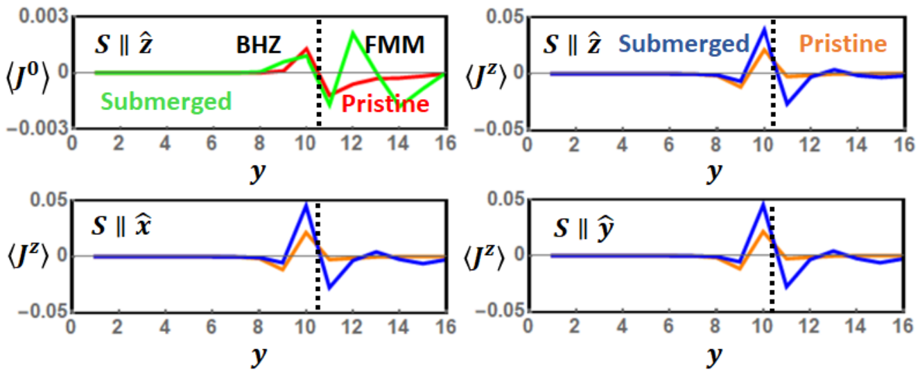
The longitudinal charge current as a function of transverse coordinate $\langle J^{0}(y)\rangle$ is shown in Fig. 3, which features a laminar current whose direction of flow depends on $y$. The net current vanishes up to numerical precision, in accordance with Eq. (8). The local charge current is finite only when the magnetization has an out-of-plane component $S_{z}$, a feature inherited from the asymmetric band structure. Moreover, the current is nonzero only when the BHZ and FMM are coupled $t_{B}\neq 0$, so it is entirely proximity induced. A close inspection reveals that both the charge and spin currents arise from contributions not only from the edge states, but from all the subbands. This makes the currents easily persist up to room temperature, which is an advantage over that induced at the topological superconductor/FMM interfaceBrydon et al. 2013; Schnyder et al. 2013. For our choice of parameters, the magnitude of the current is of the order of $\langle J^{0}(y)\rangle\sim 10^{-3}et/\hbar\sim 10^{-7}$A, and the flow direction alternates between $+{\hat{\bf x}}$ and $-{\hat{\bf x}}$ at the length scale of lattice constant $\sim$nm. The Ampere’s circuital law $B=\mu_{0}\langle J^{0}(y)\rangle/2\pi r$ then indicates that at a distance $r\sim$nm above the surface, the laminar current produces a magnetic field $\sim 1$Oe that points along ${\hat{\bf y}}$ and alternates at the length scale of nm. Thus although the laminar current is not expected to manifest in the transport properties, the alternating magnetic field it produces should in principle be measurable.

Concerning the spin current, we first remark that the BHZ model alone does not produce a net edge spin current if the Dirac point locates at the chemical potential. This is because the spin current caused by the edge state is canceled out by the contribution from the BHZ valence bands that are also spin polarized. To elaborate this statement, in Fig. 4 (a) we show the dispersion of the BHZ ribbon, with the red and blue colors indicating the spin polarization of the eigenstates $|k_{x},n_{y}\rangle$ near the $y=1$ edge

The Dirac cone has the spin up propagating with positive group velocity and spin down with negative group velocity at the $y=1$ edge, as expected. In addition to this, one sees that the valence bands are also spin polarized (so are the conduction bands, but they are not important due to the Fermi distribution). Moreover, at least some parts of the valence bands have spin up but negative group velocity (red color and negative slope in Fig. 4 (a)), meaning that these states produce a spin current against that produced by the edge states. The same mechanism also happens at the other edge $y=10$.

To quantify the contribution to the edge current from the Dirac cone and that from the valence bands, we calculate the spin current in the lattice model by summing the states within an energy window $E_{cut}$ around the chemical potential

where $\theta(E_{cut}-|E_{n}|)$ is the step function. As shown in Fig. 4 (b), the $E_{cut}=1$ case that includes only the Dirac cone contribution has a finite spin current, but the $E_{cut}=8$ case that sums over the entire band structure gives a zero spin current. In other words, the contribution from the bulk bands cancels out that from the edge state Dirac cone to yield a zero spin current. A finite spin current occurs only when the Dirac point is shifted away from the chemical potential, or in a certain experiment that can measure the equilibrium spin current contributed only within an energy window near the chemical potentialChen 2020a.

On the other hand, when the BHZ model is made in conjunction with an FMM, a persistent spin current is produced for both the pristine and the submerged cases, and is a laminar flow that percolates into the FMM, as shown in Fig. 3. Such a laminar spin current appears regardless of the direction of the magnetization and the energy of the Dirac point. The magnitude of the profile of the spin current only differ by about $20\%$ at different magnetization directions, as can be seen by comparing the $\langle J^{z}\rangle$ as a function of $y$ at ${\bf S}\parallel{\hat{\bf x}}$, ${\bf S}\parallel{\hat{\bf y}}$, and ${\bf S}\parallel{\hat{\bf z}}$ in Fig. 3.

The components $b=\left\{x,y,z\right\}$ of the spin polarization induced by a longitudinal electric field $E(i,t){\hat{\bf x}}$

in our lattice model can be formulated within a linear response theory, where the real part of the DC magnetoelectric susceptibility is calculated byChen et al. 2009; Takigawa et al.

as detailed in Appendix B. The function $\tilde{F}(E_{n},E_{m})$ is highly peaked at $E_{n}\approx E_{m}\approx 0$, meaning that the states at the Fermi surface contribute the most to the response, as expected, which include both the Dirac cone-like bands and the FMM-like subbands according to Fig. 1 (c) and (d). We focus on the DC magnetoelectric susceptibility $\lim_{\omega\rightarrow 0}{\rm Re}\chi^{b}(i,\omega)\equiv\chi^{b}(y)$ as a function of transverse coordinate $y$. We also remark that a recent work in magnetized BHZ model suggests that a damping-like spin torque can be induced by impuritiesGhosh and Manchon 2017. This feature is analogous to the spin mixing enhanced by disorder-induced spin-dependent scattering originally uncovered in metallic spin valves and domain wallsZhang et al. 2002; Zhang and Li 2004. Motivated by these earlier works, and also for the sake of removing the numerical ambiguities detailed in Appendix B, we add random impurities into the BHZ/FMM junction

where $i\in imp$ denotes the impurity sites. We choose a relatively large impurity potential $U_{imp}=4$ and density $n_{imp}=10\%$ in an attempt to draw relevance to TMD-based 2D TIs, where a significant amount of defects, such as missing sulfur atoms, are known to be a realistic issueLiu et al. 2013; Hong et al. 2015; Lin et al. 2016; Vancsó et al. 2016. The magnetoelectric susceptibility $\chi^{b}$ is then calculated by Eq. (14) using the lattice eigenstates $|n\rangle$.

The result for the magnetization directions ${\bf S}\parallel{\hat{\bf z}}$ and ${\bf S}\parallel{\hat{\bf x}}$ is shown in Fig. 5, where the magnetoelectric susceptibility averaged over the longitudinal direction $\chi^{z}(y)\equiv\sum_{x=1}^{N_{x}}\chi^{z}(x,y)/N_{x}$ for a specific impurity configuration is presented. The nonzero $\chi^{z}(y)$ near the free edge $y=1$ delineates the Edelstein effect of the BHZ model alone, i.e., current induced spin polarization caused by the edge state, analogous to that occurs in 3D TIsTian et al. 2015; Kondou et al. 2016; Liu et al. 2018; Dankert et al. 2018; Chen 2020b. At mean free time $\tau\sim 10^{-14}$s and a typical experimental electric field strength $E\sim 10^{4}$kgm/Cs², the induced spin polarization at the free edge is of the order of $10^{-7}$ (in units of $\mu_{B}$). In contrast, at the $y=10$ edge where the BHZ model is made in contact with the FMM, the magnitude of $\chi^{z}(y)$ is enhanced at small interface hopping $t_{B}=0.2$ but decreases at larger $t_{B}$. The spatial profile of $\chi^{z}(y)$ extends into the FMM for both the pristine and the submerged situations, and changes with $t_{B}$ in a rather complicated manner. The band structures in Fig. 1 (c) and (d) naturally explain this enhancement of $\chi^{z}(y)$ due to interface hopping: Compared to an isolated BHZ model, the BHZ/FMM junction has many additional FMM states at the chemical potential ($|n\rangle$ and $|m\rangle$ in Eq. (14)) that participate in the particle-hole excitation process of the magnetoelectric response. Moreover, the FMM wave functions and the edge state wave functions have a significant overlap due to percolation of the edge state, yielding nonzero matrix elements $\langle n|{\hat{O}}|m\rangle$ in Eq. (14). Notice that an isolated FMM does not exhibit Edelstein effect, so the nonzero $\chi^{z}(y)$ in the FMM region $y\in FM$ entirely originates from the proximity to the BHZ model.

The average magnetoelectric susceptibility in the FMM region $\chi^{b}_{F}\equiv\sum_{y\in FM}\chi^{b}(y)/N_{y,FM}$ is what yields the spin torque on the magnetization ${\bf S}$. Since the current-induced spin polarization is polarized along ${\hat{\bf z}}$ for an isolated BHZ model, it is customary to define the field-like torque in the FMM to be along ${\hat{\bf S}}\times{\hat{\bf z}}$ and the damping-like torque to be along ${\hat{\bf S}}\times({\hat{\bf S}}\times{\hat{\bf z}})$, as in the usual metallic thin film spin-transfer torque (STT) devices. We find that if the magnetization lies in the $xy$-plane or entirely points along ${\hat{\bf z}}$, then out of the three components ${\chi}_{F}^{b}=\left\{\chi_{F}^{x},\chi_{F}^{y},\chi_{F}^{z}\right\}$ only $\chi_{F}^{z}$ is nonzero. This indicates that the spin torque is entirely field-like if the magnetization lies in the $xy$-plane, and there is no torque if the magnetization points out-of-plane ${\bf S}\parallel{\hat{\bf z}}$. For magnetization along other directions, a small damping-like component develops (note that our calculation neglects other complications such as spin-orbit torqueManchon and Zhang 2008; Manchon and Zhang 2009 and spin relaxation). This is very different from the STT in usual metallic heterostructuresBerger 1996; Slonczewski 1996 or that induced by the spin Hall effectChen et al. 2015; Sakanashi et al. 2018, where the plane wave states usually contribute to both field-like and damping-like torque at any magnetization direction.

Figure 6 shows the result for the magnetization direction ${\bf S}\parallel{\hat{\bf x}}+{\hat{\bf z}}$, which has both the field-like $\chi^{z}$ and damping-like $\chi^{y}$ components. We find that the damping-like component is generally one order of magnitude smaller than the field-like component. A closer investigation shows that near the two edges of the BHZ region, both $\chi^{z}$ and $\chi^{y}$ are locally enhanced by the impurities, as can be seen from the local $\left\{\chi^{y},\chi^{z}\right\}$ map in Fig. 6. On the other hand, in the FMM region, the magnitude of both components does not seem to correlate with impurity positions. These features are true for both the pristine and the submerged types of band structures. At a typical external electric current $j_{c}\sim 10^{11}$A/m², the spin polarization obtained from Eq. (13) yields a spin torque according to the Landau-Lifshitz dynamics

which is basically the numerical values of $\chi^{b}_{F}$ multiplied by GHz, as demonstrated in Appendix B. The absolute magnitude of the spin torque is fairly consistent with that uncovered experimentallyShao et al. 2016; Zhang et al. 2016; Mendes et al. 2018; Bansal et al. 2019; Wu et al. 2020; Fan et al. 2020, although one should keep in mind that our BHZ/FMM side junction is different from the experimental setup where the TMD is usually deposit on top of the FMM thin film.

References

- Kane and Mele (2005) C. L. Kane and E. J. Mele, Phys. Rev. Lett. 95, 226801 (2005).
- Bernevig et al. (2006) B. A. Bernevig, T. L. Hughes, and S.-C. Zhang, Science 314, 1757 (2006).
- Bernevig and Zhang (2006) B. A. Bernevig and S.-C. Zhang, Phys. Rev. Lett. 96, 106802 (2006).
- König et al. (2007) M. König, S. Wiedmann, C. Brüne, A. Roth, H. Buhmann, L. W. Molenkamp, X.-L. Qi, and S.-C. Zhang, Science 318, 766 (2007).
- König et al. (2008) M. König, H. Buhmann, L. W. Molenkamp, T. Hughes, C.-X. Liu, X.-L. Qi, and S.-C. Zhang, J. Phys. Soc. Jpn. 77, 031007 (2008).
- Mellnik et al. (2014) A. R. Mellnik, J. S. Lee, A. Richardella, J. L. Grab, P. J. Mintun, M. H. Fischer, A. Vaezi, A. Manchon, E.-A. Kim, N. Samarth, and D. C. Ralph, Nature 511, 449 (2014).
- Mahendra et al. (2018) D. C. Mahendra, R. Grassi, J.-Y. Chen, M. Jamali, D. Reifsnyder Hickey, D. Zhang, Z. Zhao, H. Li, P. Quarterman, Y. Lv, M. Li, A. Manchon, K. A. Mkhoyan, T. Low, and J.-P. Wang, Nat. Mater. 17, 800 (2018).
- Shiomi et al. (2014) Y. Shiomi, K. Nomura, Y. Kajiwara, K. Eto, M. Novak, K. Segawa, Y. Ando, and E. Saitoh, Phys. Rev. Lett. 113, 196601 (2014).
- Rojas-Sánchez et al. (2016) J.-C. Rojas-Sánchez, S. Oyarzún, Y. Fu, A. Marty, C. Vergnaud, S. Gambarelli, L. Vila, M. Jamet, Y. Ohtsubo, A. Taleb-Ibrahimi, P. Le Fèvre, F. Bertran, N. Reyren, J.-M. George, and A. Fert, Phys. Rev. Lett. 116, 096602 (2016).
- Mendes et al. (2017) J. B. S. Mendes, O. Alves Santos, J. Holanda, R. P. Loreto, C. I. L. de Araujo, C.-Z. Chang, J. S. Moodera, A. Azevedo, and S. M. Rezende, Phys. Rev. B 96, 180415 (2017).
- Yokoyama et al. (2010) T. Yokoyama, J. Zang, and N. Nagaosa, Phys. Rev. B 81, 241410 (2010).
- Sakai and Kohno (2014) A. Sakai and H. Kohno, Phys. Rev. B 89, 165307 (2014).
- Fischer et al. (2016) M. H. Fischer, A. Vaezi, A. Manchon, and E.-A. Kim, Phys. Rev. B 93, 125303 (2016).
- Ndiaye et al. (2017) P. B. Ndiaye, C. A. Akosa, M. H. Fischer, A. Vaezi, E.-A. Kim, and A. Manchon, Phys. Rev. B 96, 014408 (2017).
- Okuma and Nomura (2017) N. Okuma and K. Nomura, Phys. Rev. B 95, 115403 (2017).
- Ghosh and Manchon (2018) S. Ghosh and A. Manchon, Phys. Rev. B 97, 134402 (2018).
- Shao et al. (2016) Q. Shao, G. Yu, Y.-W. Lan, Y. Shi, M.-Y. Li, C. Zheng, X. Zhu, L.-J. Li, P. K. Amiri, and K. L. Wang, Nano Lett. 16, 7514 (2016).
- Zhang et al. (2016) W. Zhang, J. Sklenar, B. Hsu, W. Jiang, M. B. Jungfleisch, J. Xiao, F. Y. Fradin, Y. Liu, J. E. Pearson, J. B. Ketterson, Z. Yang, and A. Hoffmann, APL Mater. 4, 032302 (2016).
- Mendes et al. (2018) J. B. S. Mendes, A. Aparecido-Ferreira, J. Holanda, A. Azevedo, and S. M. Rezende, Appl. Phys. Lett. 112, 242407 (2018).
- Bansal et al. (2019) R. Bansal, A. Kumar, N. Chowdhury, N. Sisodia, A. Barvat, A. Dogra, P. Pal, and P. Muduli, J. Magn. Magn. Mater. 476, 337 (2019).
- Wu et al. (2020) G. Wu, Y. Ren, X. He, Y. Zhang, H. Xue, Z. Ji, Q. Y. Jin, and Z. Zhang, Phys. Rev. Applied 13, 024027 (2020).
- Fan et al. (2020) Y. Fan, H. Li, M. DC, T. Peterson, J. Held, P. Sahu, J. Chen, D. Zhang, A. Mkhoyan, and J.-P. Wang, APL Materials 8, 041102 (2020).
- Qian et al. (2014) X. Qian, J. Liu, L. Fu, and J. Li, Science 346, 1344 (2014).
- Ma et al. (2015) Y. Ma, L. Kou, X. Li, Y. Dai, S. C. Smith, and T. Heine, Phys. Rev. B 92, 085427 (2015).
- Wu et al. (2018) S. Wu, V. Fatemi, Q. D. Gibson, K. Watanabe, T. Taniguchi, R. J. Cava, and P. Jarillo-Herrero, Science 359, 76 (2018).
- Bernevig and Hughes (2013) B. A. Bernevig and T. L. Hughes, Topological Insulators and Topological Superconductors (Princeton University Press, 2013).
- Cowley and Sze (1965) A. M. Cowley and S. M. Sze, J. Appl. Phys. 36, 3212 (1965).
- Tung (2014) R. T. Tung, Appl. Phys. Rev. 1, 011304 (2014).
- Gambardella and Miron (2011) P. Gambardella and I. M. Miron, Phil. Trans. R. Soc. A 369, 3175 (2011).
- Chen and Schnyder (2015) W. Chen and A. P. Schnyder, Phys. Rev. B 92, 214502 (2015).
- Nagaosa (2008) N. Nagaosa, Journal of the Physical Society of Japan 77, 031010 (2008).
- Brydon et al. (2013) P. M. R. Brydon, C. Timm, and A. P. Schnyder, New J. Phys. 15, 045019 (2013).
- Schnyder et al. (2013) A. P. Schnyder, C. Timm, and P. M. R. Brydon, Phys. Rev. Lett. 111, 077001 (2013).
- Chen (2020a) W. Chen, Phys. Rev. B 101, 195120 (2020a).
- Chen et al. (2009) W. Chen, B. M. Andersen, and P. J. Hirschfeld, Phys. Rev. B 80, 134518 (2009).
- (36) M. Takigawa, M. Ichioka, and K. Machida, Eur. Phys. J. B 27, 303.
- Ghosh and Manchon (2017) S. Ghosh and A. Manchon, Phys. Rev. B 95, 035422 (2017).
- Zhang et al. (2002) S. Zhang, P. M. Levy, and A. Fert, Phys. Rev. Lett. 88, 236601 (2002).
- Zhang and Li (2004) S. Zhang and Z. Li, Phys. Rev. Lett. 93, 127204 (2004).
- Liu et al. (2013) D. Liu, Y. Guo, L. Fang, and J. Robertson, Applied Physics Letters 103, 183113 (2013).
- Hong et al. (2015) J. Hong, Z. Hu, M. Probert, K. Li, D. Lv, X. Yang, L. Gu, N. Mao, Q. Feng, L. Xie, J. Zhang, D. Wu, Z. Zhang, C. Jin, W. Ji, X. Zhang, J. Yuan, and Z. Zhang, Nat. Commun. 6, 6293 (2015).
- Lin et al. (2016) Z. Lin, B. R. Carvalho, E. Kahn, R. Lv, R. Rao, H. Terrones, M. A. Pimenta, and M. Terrones, 2D Mater. 3, 022002 (2016).
- Vancsó et al. (2016) P. Vancsó, G. Z. Magda, J. Pető, J.-Y. Noh, Y.-S. Kim, C. Hwang, L. P. Biró, and L. Tapasztó, Sci. Rep. 6, 29726 (2016).
- Tian et al. (2015) J. Tian, I. Miotkowski, S. Hong, and Y. P. Chen, Sci. Rep. 5, 14293 (2015).
- Kondou et al. (2016) K. Kondou, R. Yoshimi, A. Tsukazaki, Y. Fukuma, J. Matsuno, K. S. Takahashi, M. Kawasaki, Y. Tokura, and Y. Otani, Nat. Phys. 12, 1027 (2016).
- Liu et al. (2018) Y. Liu, J. Besbas, Y. Wang, P. He, M. Chen, D. Zhu, Y. Wu, J. M. Lee, L. Wang, J. Moon, N. Koirala, S. Oh, and H. Yang, Nat. Commun. 9, 2491 (2018).
- Dankert et al. (2018) A. Dankert, P. Bhaskar, D. Khokhriakov, I. H. Rodrigues, B. Karpiak, M. V. Kamalakar, S. Charpentier, I. Garate, and S. P. Dash, Phys. Rev. B 97, 125414 (2018).
- Chen (2020b) W. Chen, J. Phys. Condens. Matter 32, 035809 (2020b).
- Manchon and Zhang (2008) A. Manchon and S. Zhang, Phys. Rev. B 78, 212405 (2008).
- Manchon and Zhang (2009) A. Manchon and S. Zhang, Phys. Rev. B 79, 094422 (2009).
- Berger (1996) L. Berger, Phys. Rev. B 54, 9353 (1996).
- Slonczewski (1996) J. Slonczewski, J. Magn. Magn. Mater. 159, L1 (1996).
- Chen et al. (2015) W. Chen, M. Sigrist, J. Sinova, and D. Manske, Phys. Rev. Lett. 115, 217203 (2015).
- Sakanashi et al. (2018) K. Sakanashi, M. Sigrist, and W. Chen, J. Phys. Condens. Matter 30, 205803 (2018).