Distributed Stochastic Algorithms for High-rate Streaming Principal Component Analysis
Abstract
This paper considers the problem of estimating the principal eigenvector of a covariance matrix from independent and identically distributed data samples in streaming settings. The streaming rate of data in many contemporary applications can be high enough that a single processor cannot finish an iteration of existing methods for eigenvector estimation before a new sample arrives. This paper formulates and analyzes a distributed variant of the classical Krasulina’s method (D-Krasulina) that can keep up with the high streaming rate of data by distributing the computational load across multiple processing nodes. The analysis shows that—under appropriate conditions—D-Krasulina converges to the principal eigenvector in an order-wise optimal manner; i.e., after receiving samples across all nodes, its estimation error can be . In order to reduce the network communication overhead, the paper also develops and analyzes a mini-batch extension of D-Krasulina, which is termed DM-Krasulina. The analysis of DM-Krasulina shows that it can also achieve order-optimal estimation error rates under appropriate conditions, even when some samples have to be discarded within the network due to communication latency. Finally, experiments are performed over synthetic and real-world data to validate the convergence behaviors of D-Krasulina and DM-Krasulina in high-rate streaming settings.
keywords
Distributed algorithms; Krasulina’s method; mini-batch optimization; principal component analysis; stochastic methods1 Introduction
Dimensionality reduction and feature learning methods such as principal component analysis (PCA), sparse PCA, independent component analysis, and autoencoder form an important component of any machine learning pipeline. For data lying in a -dimensional space, such methods try to find the variables/features that are most relevant for solving an application-specific task (e.g., classification, regression, estimation, data compression, etc.). The focus of this work is on PCA, where the objective is to compute -features that capture most of the variance in data. The proliferation of big data (both in terms of dimensionality and number of samples) has resulted in an increased interest in developing new algorithms for PCA due to the fact that classical numerical solutions (e.g., power iteration and Lanczos method (Golub and Van Loan 2012)) for computing eigenvectors of symmetric matrices do not scale well with high dimensionality and large sample sizes. The main interest in this regard has been on developing algorithms that are cheap in terms of both memory and computational requirements as a function of dimensionality and number of data samples.
In addition to high dimensionality and large number of samples, another defining characteristic of modern data is their streaming nature in many applications; examples of such applications include the internet-of-things, high-frequency trading, meteorology, video surveillance, autonomous vehicles, social media analytics, etc. Several stochastic methods have been developed in the literature to solve the PCA problem in streaming settings (Krasulina 1969; Oja and Karhunen 1985; Sanger 1989; Warmuth and Kuzmin 2007; Zhang and Balzano 2016). These methods operate under the implicit assumption that the data arrival rate is slow enough so that each sample can be processed before the arrival of the next one. But this may not be true for many modern applications involving high-rate streaming data. To overcome this obstacle corresponding to high-rate streaming data, this paper proposes and analyzes distributed and distributed, mini-batch variants of the classical Krasulina’s method (Krasulina 1969). Before providing details of the proposed methods and their relationship to prior work, we provide a brief overview of the streaming PCA problem.
1.1 Principal Component Analysis (PCA) from Streaming Data
For data lying in , PCA learns a -dimensional subspace with maximum data variance. Let be a random vector that is drawn from some unknown distribution with zero mean and covariance matrix. For the constraint set , we can pose PCA as the following constrained optimization problem:
| (1) |
where denotes the trace operator. The solution for the statistical risk maximization problem (1) is the matrix with top eigenvectors of . In practice, however, (1) cannot be solved in its current form since is unknown. But if we have data samples, , drawn independently from , then we can accumulate these data samples to calculate the sample covariance matrix as:
| (2) |
where . Instead of solving (1), we can now solve an empirical risk maximization problem
| (3) |
In principle, we can solve (3) by computing the singular value decomposition (SVD) of sample covariance . But this is a computationally intensive task that requires multiplications and that has a memory overhead of . In contrast, the goal in high-dimensional PCA problems is often to have computational complexity and memory complexity (Li et al. 2016).
More efficient (and hence popular) approaches for PCA use methods such as the power/orthogonal iteration and Lanczos method (Golub and Van Loan 2012, Chapter 8). Although these methods improve overall computational complexity of PCA to , they still have memory requirements on the order of . In addition, these are batch methods that require computing the sample covariance matrix , which results in multiplication operations. Further, in streaming settings where the goal is real-time decision making from data, it is infeasible to compute . Because of these reasons, stochastic approximation methods such as Krasulina’s method (Krasulina 1969) and Oja’s rule (Oja and Karhunen 1985) are often favored for the PCA problem. Both these are simple and extremely efficient algorithms, achieving computational and memory complexity per iteration, for computing the principal eigenvector (i.e., ) of a covariance matrix in streaming settings. Recent years in particular have seen an increased popularity of these algorithms and we will discuss these recent advances in Section 1.3.
Both Oja’s rule and Krasulina’s method share many similarities. In this paper, we focus on Krasulina’s method with the understanding that our findings can be mapped to Oja’s rule through some tedious but straightforward calculations. Using for algorithmic iteration, Krasulina’s method estimates the top eigenvector by processing one data sample in each iteration as follows:11 1 In contrast, the iterate of Oja’s rule is given by
| (4) |
where denotes the step size. Going forward, we will be using in place of in expressions such as (4) for notational compactness. In practice, however, one should neither explicitly store nor explicitly use it for calculation purposes.
Note that one can interpret Krasulina’s method as a solution to an optimization problem. Using Courant–Fischer Minimax Theorem (Golub and Van Loan 2012, Theorem 8.1.2), the top eigenvector computation (i.e., 1-PCA, which is the version of (1)) can be posed as the following optimization problem:
| (5) |
In addition, the gradient of the function defined in (5) is:
| (6) |
Looking at (4)–(6), we see that (4) is very similar to applying stochastic gradient descent (SGD) to the nonconvex problem (5), with the only difference being the scaling factor of . Nonetheless, since (5) is a nonconvex problem and we are interested in global convergence behavior of Krasulina’s method, existing tools for analysis of the standard SGD problem (Bottou 2010; Recht et al. 2011; Dekel et al. 2012; Reddi et al. 2016b; Reddi et al. 2016c) do not lend themselves to the fastest convergence rates for Krasulina’s method. Despite its nonconvexity, however, (5) has a somewhat benign optimization landscape and a whole host of algorithmic techniques and analytical tools have been developed for such structured nonconvex problems in recent years that guarantee fast convergence to a global solution. In this paper, we leverage some of these recent developments to guarantee near-optimal global convergence of two variants of Krasulina’s method in the case of high-rate streaming data.
Before proceeding further, it is worth noting that while Krasulina’s method primarily focuses on the 1-PCA problem, it can be used to solve the -PCA problem. But such an indirect approach, which involves repeated use of the Krasulina’s method times, can be inefficient in terms of sample complexity (Allen-Zhu and Li 2017a, Section 1). We leave investigation of a near-optimal direct method for the -PCA problem involving high-rate streaming data for future work.
1.2 Our Contributions
In this paper, we propose and analyze two distributed variants of Krasulina’s method for estimating the top eigenvector of a covariance matrix from fast streaming, independent and identically distributed (i.i.d.) data samples. Our theoretical analysis, as well as numerical experiments on synthetic and real data, establish near-optimality of the proposed algorithms. In particular, our analysis shows that the proposed algorithms can achieve the optimal convergence rate of for 1-PCA after processing a total of data samples (see (Jain et al. 2016, Theorem 1.1) and (Allen-Zhu and Li 2017a, Theorem 6)). In terms of details, following are our key contributions:
- 1.
Our first contribution corresponds to the scenario in which there is a mismatch of between the data streaming rate and the processing capability of a single processor, i.e., one iteration of Krasulina’s method on one processor takes as long as data arrival epochs. Our solution to this problem, which avoids discarding of samples, involves splitting the data stream into parallel streams that are then input to interconnected processors. Note that this splitting effectively reduces the streaming rate at each processor by a factor of . We then propose and analyze a distributed variant of Krasulina’s method—termed D-Krasulina—that solves the 1-PCA problem for this distributed setup consisting of processing nodes. Our analysis shows that D-Krasulina can result in an improved convergence rate of after iterations (Theorem 7), as opposed to the rate for the classical Krasulina’s method at any one of the nodes seen in isolation. Establishing this result involves a novel analysis of Krasulina’s method that brings out the dependence of its convergence rate on the variance of the sample covariance matrix; this analysis coupled with a variance reduction argument leads to the convergence rate of for D-Krasulina under appropriate conditions.
- 2.
Mini-batching of data samples has long been promoted as a strategy in stochastic methods to reduce the wall-clock time. Too large of a mini-batch, however, can have an adverse effect on the algorithmic performance; see, e.g., (Shamir and Srebro 2014, Sec. VIII). One of the challenges in mini-batched stochastic methods, therefore, is characterizing the mini-batch size that leads to near-optimal convergence rates in terms of the number of processed samples. In (Agarwal and Duchi 2011; Cotter et al. 2011; Dekel et al. 2012; Shamir and Srebro 2014; Ruder 2016; Golmant et al. 2018; Goyal et al. 2017), for example, the authors have focused on this challenge for the case of mini-batch SGD for convex and nonconvex problems. In the case of nonconvex problems, however, the guarantees only hold for convergence to first-order stationary points. In contrast, our second contribution is providing a comprehensive understanding of the global convergence behavior of mini-batch Krasulina’s method. In fact, our analysis of D-Krasulina is equivalent to that of a mini-batch (centralized) Krasulina’s method that uses a mini-batch of samples in each iteration. This analysis, therefore, already guarantees near-optimal convergence rate with arbitrarily high probability, as opposed to probability for (Yang et al. 2018), for an appropriately mini-batched Krasulina’s method in a centralized setting. In addition, in the case of high-rate streaming data that requires splitting the data stream into parallel ones, we characterize the global convergence behavior of a mini-batch generalization of D-Krasulina—termed DM-Krasulina—in terms of the mini-batch size. This involves specifying the conditions under which mini-batches of size per node can lead to near-optimal convergence rate of after iterations of DM-Krasulina (Theorem 11). An implication of this analysis is that for a fixed (network-wide) sample budget of samples, DM-Krasulina can achieve rate after iterations provided the (network-wide) mini-batch size satisfies for some constant (Corollary 12).
- 3.
Our next contribution is an extended analysis of DM-Krasulina that concerns the scenario where (computational and/or communication) resource constraints translate into individual nodes still receiving more data samples than they can process in one iteration of DM-Krasulina. This resource-constrained setting necessitates DM-Krasulina dropping samples across the network in each iteration. Our analysis in this setting shows that such loss of samples need not result in sub-optimal performance. In particular, DM-Krasulina can still achieve near-optimal convergence rate as a function of the number of samples arriving in the network—for both infinite-sample and finite-sample regimes—as long as (Corollary 13).
- 4.
We provide numerical results involving both synthetic and real-world data to establish the usefulness of the proposed algorithms, validate our theoretical analysis, and understand the impact of the number of dropped samples per iteration of DM-Krasulina on the convergence rate. These results in particular corroborate our findings that increasing the mini-batch size improves the performance of DM-Krasulina up to a certain point, after which the convergence rate starts to decrease.
1.3 Related Work
Solving the PCA problem efficiently in a number of settings has been an active area of research for decades. (Krasulina 1969; Oja and Karhunen 1985) are among the earliest and most popular methods to solve PCA in streaming data settings. Several variants of these methods have been proposed over the years, including (Bin Yang 1995; Chatterjee 2005; Doukopoulos and Moustakides 2008). Like earlier developments in stochastic approximation methods (Robbins and Monro 1951), such variants were typically shown to converge asymptotically. Convergence rate analyses for stochastic optimization in finite-sample settings (Shapiro and Homem-de Mello 2000; Linderoth et al. 2006) paved the way for non-asymptotic convergence analysis of different variants of the stochastic PCA problem, which is fundamentally a nonconvex optimization problem. Because of the vastness of literature on (stochastic) PCA, this work is tangentially or directly related to a number of such prior works. We review some of these works in the following under the umbrellas of different problem setups, with the understanding that the resulting lists of works are necessarily incomplete. Much of our discussion in the following focuses on solving the PCA problem in (fast) streaming and distributed data settings, which is the main theme in this paper.
Sketching for PCA. Sketching methods have long been studied in the literature for solving problems involving matrix computations; see (Woodruff 2014) for a review of such methods. The main idea behind these methods is to compress data using either randomized or deterministic sketches and then perform computations on the resulting low-dimensional data. While sketching has been used as a tool to solve the PCA problem in an efficient manner (see, e.g., (Warmuth and Kuzmin 2007; Halko et al. 2011; Liberty 2013; Leng et al. 2015; Karnin and Liberty 2015)), the resulting methods cannot be used to exactly solve (1) in the fast streaming settings of this paper.
Online PCA. The PCA problem has also been extensively studied in online settings. While such settings also involve streaming data, the main goal in online PCA is to minimize the cumulative subspace estimation error over the entire time horizon of the algorithm. The online PCA framework, therefore, is especially useful in situations where either the underlying subspace changes over time or there is some adversarial noise in the sampling process. Some of the recent works in this direction include (Garber et al. 2015; Allen-Zhu and Li 2017b; Garber 2018; Marinov et al. 2018; Kotłowski and Neu 2019).
Stochastic convex optimization for PCA. One approach towards solving (3) in streaming settings is to relax the PCA problem to a convex optimization problem and then use SGD to solve the resulting stochastic convex optimization problem (Arora et al. 2013; Garber and Hazan 2015; Nie et al. 2016). The benefit of this approach is that now one can rely on rich literature for solving stochastic convex problems using SGD. But the tradeoff is that one now needs to store an iterate of dimension , as opposed to an iterate of dimension when we solve the PCA problem in its original nonconvex form. Due to these high memory requirements of , we limit ourselves to solving PCA in the nonconvex form.
Streaming PCA and nonconvex optimization. The PCA problem in the presence of streaming data can also be tackled as an explicit constrained nonconvex optimization program (Zhang and Balzano 2016; De Sa et al. 2015). In (Zhang and Balzano 2016), for instance, the problem is solved as an optimization program over the Grassmannian manifold. The resulting analysis, however, relies on the availability of a good initial guess. In contrast, the authors in (De Sa et al. 2015) analyze the use of the SGD for solving certain nonconvex problems that include PCA. The resulting approach, however, requires the step size to be a significantly small constant for eventual convergence (e.g., for the Netflix Prize dataset); this translates into slower convergence in practice.
Classical stochastic approximation methods for PCA. Recent years have seen an increased interest in understanding the global convergence behavior of classical stochastic approximation methods such as Krasulina’s method (Krasulina 1969) and Oja’s rule (Oja and Karhunen 1985) for the PCA problem in non-asymptotic settings (Allen-Zhu and Li 2017a; Chatterjee 2005; Hardt and Price 2014; Shamir 2015; Shamir 2016; Jain et al. 2016; Li et al. 2016; Tang 2019; Henriksen and Ward 2019; Amid and Warmuth 2019). Some of these works, such as (Shamir 2015) and (Shamir 2016), use variance reduction techniques to speed-up the algorithmic convergence. Such works, however, require multiple passes over the data, which makes them ill-suited for fast streaming settings. The analysis in (Shamir 2015) and (Shamir 2016) also requires an initialization close to the true subspace, which is somewhat unlikely in practice. Among other works, the authors in (Allen-Zhu and Li 2017a) provide eigengap-free convergence guarantees for Oja’s rule. Since the results in this work do not take into account the variance of data samples, they do not generalize to mini-batch/distributed streaming settings. The authors in (Jain et al. 2016) do provide variance-dependent guarantees for Oja’s rule, which makes this work the most relevant to ours. In particular, the authors in (Yang et al. 2018) have extended the initial analysis in (Jain et al. 2016) to mini-batch settings. However, the results derived in (Yang et al. 2018) only hold with probability , which is in sharp contrast to the results of this paper. Note that while one could increase the probability of success in (Yang et al. 2018) through multiple algorithmic runs, this is not a feasible strategy in streaming settings.
Distributed PCA and streaming data. Several recent works such as (Balcan et al. 2016; Boutsidis et al. 2016; Garber et al. 2017; De Sa et al. 2018) have focused on the PCA problem in distributed settings. Among these works, the main focus in (Balcan et al. 2016; Boutsidis et al. 2016; Garber et al. 2017) is on improving the communications efficiency. This is accomplished in (Balcan et al. 2016; Boutsidis et al. 2016) by sketching the local iterates and communicating the resulting compressed iterates to a central server in each iteration. In contrast, Garber et al. 2017 provides a batch solution in which every node in the network first computes the top eigenvector of its local (batch) covariance matrix and then, as a last step of the algorithm, all the local eigenvector estimates are summed up at a central server to provide an eigenvector estimate for the global covariance matrix. In contrast to these works, our focus in this paper is on establishing that distributed (mini-batch) variants of stochastic approximation methods such as Oja’s rule and Krasulina’s method can lead to improved convergence rates, as a function of the number of samples, for the PCA problem in fast streaming settings. In this regard, our work is more closely related to (De Sa et al. 2018), where the authors use the momentum method to accelerate convergence of power method and further extend their work to stochastic settings. However, the approach of (De Sa et al. 2018) relies on a variance reduction technique that requires a pass over the complete dataset every once in a while; this is impractical in streaming settings. In addition, theoretical guarantees in (De Sa et al. 2018) are based on the assumption of a “good” initialization; further, an implicit assumption in (De Sa et al. 2018) is that inter-node communications is fast enough that there are no communication delays.
Connections to stochastic nonconvex optimization. Recent years have also seen an increased focus on understanding (variants of) SGD for general (typically unconstrained) stochastic nonconvex optimization problems. Among such works, some have focused on classical SGD (Ge et al. 2015; Hazan et al. 2016; Hazan et al. 2017), some have studied variance-reduction variants of SGD (Reddi et al. 2016a; Reddi et al. 2016b), and some have investigated accelerated variants of stochastic nonconvex optimization (Allen-Zhu 2018b; Allen-Zhu 2018a). In particular, works such as (Reddi et al. 2016a; Allen-Zhu and Hazan 2016) are directly relevant to this paper since these works also use mini-batches to reduce sample variance and improve on SGD convergence rates. While (implicit, through the distributed framework, and explicit) mini-batching is one of the key ingredients of our work also, this paper differs from such related works because of its ability to prove convergence to a global optimum of the 1-PCA problem. In contrast, aforementioned works only provide guarantees for convergence to first-order stationary points of (typically unconstrained) stochastic nonconvex optimization problems.
1.4 Notational Convention and Paper Organization
We use lower-case (), bold-faced lower-case (), and bold-faced upper-case () letters to represent scalars, vectors, and matrices, respectively. Given a scalar and a vector , denotes the smallest integer greater than or equal to , while denotes the -norm of . Given a matrix , denotes its spectral norm and denotes its Frobenius norm. In addition, assuming to be a positive semi-definite matrix, denotes its -th largest eigenvalue, i.e., . Whenever obvious from the context, we drop from for notational compactness. Finally, denotes the expectation operator, where the underlying probability space is either implicit from the context or is explicitly pointed out in the body.
The rest of this paper is organized as follows. We first provide a formal description of the problem and the system model in Section 2. The two proposed variants of Krasulina’s method that can be used to solve the 1-PCA problem in fast streaming settings are then presented in Section 3. In Section 4, we provide theoretical guarantees for the proposed algorithms, while proofs / outlines of the proofs of the main theoretical results are provided in Section 5. Finally, numerical results using both synthetic and real-world data are presented in Section 6, while appendices are used for detailed proofs of some of the theoretical results.
2 Problem Formulation and System Model
Our goal is to use some variants of Krasulina’s method (cf. (4)) in order to obtain an estimate of the top eigenvector of a covariance matrix from independent and identically distributed (i.i.d.) data samples that are fast streaming into a system. The algorithms proposed in this regard and their convergence analysis rely on the following sets of assumptions concerning the data and the system.
2.1 Data Model
We consider a streaming data setting where a new data sample independently drawn from an unknown distribution arrives at a system at each sampling time instance . We assume a uniform data arrival rate of samples per second and, without loss of generality, take the data arrival index to be an integer. We also make the following assumptions concerning our data, which aid in our convergence analysis.
-
(Zero-mean, norm-bounded samples) Without loss of generality, the data samples have zero mean, i.e., . In addition, the data samples are almost surely bounded in norm, i.e., , where we let the bound without loss of generality.
-
(Spectral gap of the covariance matrix) The largest eigenvalue of is strictly greater than the second largest eigenvalue, i.e., .
Note that both Assumptions [ A1 ] and [ A2 ] are standard in the literature for convergence analysis of Krasulina’s method and Oja’s rule (cf. Balsubramani et al. 2013; Oja and Karhunen 1985; Allen-Zhu and Li 2017a; Jain et al. 2016).
We also associate with each data sample a rank-one random matrix , which is a trivial unbiased estimate of the population covariance matrix . We then define the variance of this unbiased estimate as follows.
Definition 1 (Variance of sample covariance matrix).
We define the variance of the sample covariance matrix as follows:
Note that all moments of the probability distribution exist by virtue of the norm boundedness of (cf. Assumption [ A1 ] ). The variance of the sample covariance matrix as defined above, therefore, exists and is finite.
The two algorithms proposed in this paper, namely, D-Krasulina and DM-Krasulina, are initialized with a random vector that is randomly generated over the unit sphere in with respect to the uniform (Haar) measure. All analysis in this paper is with respect to the natural probability space given by the stochastic process and filtered versions of this probability space.
2.2 System Model
Let denote the number of data samples that a single processing node in the system can process in one second using an iteration of the form (4). The focus of this paper is on the high-rate streaming setting, which corresponds to the setup in which the data arrival rate is strictly greater than the data processing rate . A naive approach to deal with this computation–streaming mismatch is to discard (per second) a fraction of samples in the system. Such an approach, however, leads to an equivalent reduction in the convergence rate by . We pursue an alternative to this approach in the paper that involves the simultaneous use of interconnected processors, each individually capable of processing samples per second, within the system. In particular, we advocate the use of such a network of processors in the following two manners to achieve near-optimal convergence rates (as a function of the number of samples arriving at the system) for estimates of the top eigenvector of in high-rate streaming settings.
2.2.1 Distributed Processing Over a Network of Processors
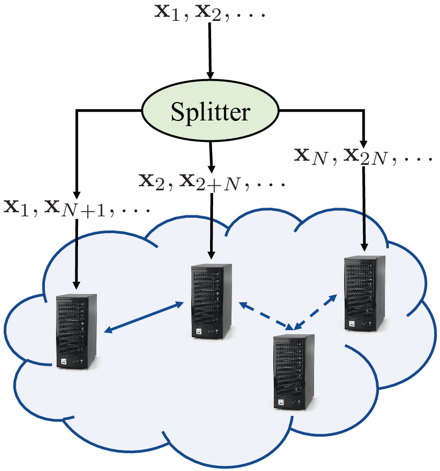
We assume the fast data stream terminates into a data splitter, which splits the original stream with data rate samples per second into parallel streams, each with data rate samples per second, that are then synchronously input to the interconnected network of processors; see Figure 1(a) for a schematic rendering of such splitting. In order to simplify notation in this setting, we reindex the data samples associated with the -th processor / data stream in the following as , where the reindexing map is simply defined as .
We also assume the network of processors implements some message passing protocol that allows it to compute sums of locally stored vectors, i.e., for the set of local vectors , within the network. This could, for instance, be accomplished using either Reduce or AllReduce primitives within most message passing implementations. We let denote the number of these primitive (sum) operations that the message passing protocol can carry out per second in the network of processors. Note that this parameter depends upon the message passing implementation, number of nodes in the network, topology of the network, and inter-node communications bandwidth, all of which are being abstracted here through .
Data splitting among this network of processors effectively slows down the data streaming rate at each processing node by a factor of . It is under this system model that we present a distributed variant of Krasulina’s method, termed D-Krasulina, in Section 3.1 that operates under the assumption of . The main analytical challenge for D-Krasulina is understanding the scenarios under which this distributed processing over a network of processors still yields near-optimal performance; we address this challenge in Section 4.1.
Remark 2.
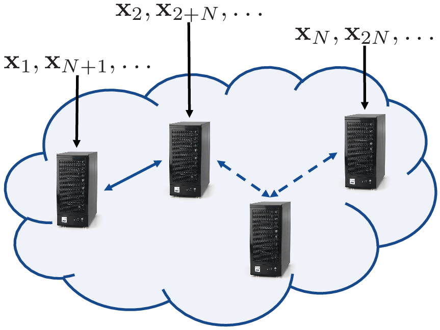
It is straightforward to see that our developments in this paper are also applicable to the setting in which data naturally arrives in a distributed manner at different nodes, as in Figure 1(b). In addition, our analysis of D-Krasulina is equivalent to that of a mini-batch Krasulina’s method running on a powerful-enough single processor that uses a mini-batch of samples in each iteration.
2.2.2 Distributed Processing Coupled with Mini-batching
Mini-batching in (centralized) stochastic methods, as discussed in Section 1.2, helps reduce the wall-clock time by reducing the number of read operations per iteration. Mini-batching of samples in distributed settings has the added advantage of reduction in the average number of primitive (sum) operations per processed sample, which further reduces the wall-clock time. It is in this vein that we put forth a mini-batched variant of D-Krasulina, which is termed DM-Krasulina, in Section 3.2.
Similar to the case of D-Krasulina (cf. Figure 1), there are several equivalent system models that can benefit from the DM-Krasulina framework. In keeping with our theme of fast streaming data, as well as for the sake of concreteness, we assume the system buffers (i.e., mini-batches) samples of the incoming data stream every seconds for some parameter . This network-wide mini-batch of samples is then split into parallel (local) mini-batches, each comprising samples, which are then synchronously input to the interconnected network of processors at a rate of samples per second and collaboratively processed by DM-Krasulina. In each iteration of DM-Krasulina, therefore, the network processes a total of samples, as opposed to samples for D-Krasulina. In order to simplify notation in this mini-batched distributed setting, we reindex the data samples in the mini-batch associated with the -th processor in iteration of DM-Krasulina as , where the reindexing map is defined as .
The DM-Krasulina framework can process all data samples arriving at the system as long as . However, when this condition is violated due to faster streaming rate , slower processing rate , slower summation rate , or any combination thereof, it becomes necessary for DM-Krasulina to discard samples at the splitter per iteration. The main analytical challenges for DM-Krasulina are, therefore, twofold: first, assuming , characterize the mini-batch size that leads to near-optimal convergence rates for DM-Krasulina in terms of the total number of samples arriving at the system; second, when discarding of samples becomes necessary, characterize the interplay between and that allows DM-Krasulina to still achieve (order-wise) near-optimal convergence rates. We address both these challenges in Section 4.2.
3 Proposed Distributed Stochastic Algorithms
We now formally describe the two stochastic algorithms, termed D-Krasulina and DM-Krasulina, that can be used to solve the 1-PCA problem from high-rate streaming data under the two setups described in Section 2.2.1 and Section 2.2.2, respectively.
3.1 Distributed Krasulina’s Method (D-Krasulina) for High-rate Streaming Data
Recall from the discussion in Section 2.2.1 that each node in the network receives data sample in iteration of the distributed implementation, which comprises processing nodes. Unlike the centralized Krasulina’s method (cf. (4)), therefore, any distributed variant of Krasulina’s method needs to process samples in every iteration . Using as a shorthand for , one natural extension of (4) that processes samples in each iteration is as follows:
| (7) |
One natural question here is whether (7) can be computed within our distributed framework. The answer to this is in the affirmative under the assumption , with the implementation (termed D-Krasulina) formally described in Algorithm 1.
Initialize: All processors initialize with randomly generated over the unit sphere
Notice that unlike classical Krasulina’s method, which processes a total of samples after iterations, D-Krasulina processes a total of samples after iterations in order to provide an estimate of the top eigenvector of . Another natural question, therefore, is whether the estimate returned by D-Krasulina can converge to at the near-optimal rate of . Convergence analysis of D-Krasulina in Section 4 establishes that the answer to this is also in the affirmative under appropriate conditions that are specified in Theorem 7. An important interpretation of this result is that our proposed distributed implementation of Krasulina’s method can lead to linear speed-up as a function of the number of processing nodes in the network.
3.2 Mini-batched D-Krasulina (DM-Krasulina) for High-rate Streaming Data
The distributed, mini-batched setup described in Section 2.2.2 entails each node receiving a mini-batch of data samples, , in each iteration , for a total of samples across the network in every iteration. Similar to (7), these samples can in principle be processed by the following variant of the original Krasulina’s iteration:
| (8) |
where is a shorthand for . Practical computation of (8) within our distributed framework, however, requires consideration of two different scenarios.
- •
Scenario 1: The mini-batched distributed framework satisfies . This enables incorporation of every sample arriving at the system into the eigenvector estimate.
- •
Scenario 2: The mini-batched distributed framework leads to the condition . This necessitates discarding of samples per iteration in the system. Stated differently, the system receives samples per iteration in this scenario, but only samples per iteration are incorporated into the eigenvector estimate.
We now formally describe the algorithm (termed DM-Krasulina) that implements (8) under both these scenarios in Algorithm 2.
Initialize: All processors initialize with randomly generated over the unit sphere
Speaking strictly in terms of implementation, the mini-batched setup of DM-Krasulina allows one to relax the condition associated with D-Krasulina to either , which still incorporates all samples into the eigenvector estimate, or , which involves discarding of samples per algorithmic iteration. While this makes DM-Krasulina particularly attractive for systems with slower communication links, the major analytical hurdle here is understanding the interplay between the different problem parameters that still allows DM-Krasulina to achieve near-optimal convergence rates in terms of the number of samples received at the system. We tease out this interplay as part of the convergence analysis of DM-Krasulina in Section 4.
4 Convergence Analysis of D-Krasulina and DM-Krasulina
Our convergence analysis of D-Krasulina and DM-Krasulina is based on understanding the rate at which the so-called potential function of these methods converges to zero as a function of the number of algorithmic iterations . Formally, this potential function is defined as follows.
Definition 3 (Potential function).
Let be the eigenvector of associated with and let be an estimate of returned by an iterative algorithm in iteration . Then the quality of the estimate can be measured in terms of the potential function that is defined as
| (9) |
Notice that is a measure of estimation error, which approaches as converges to any scalar multiple of . This measure, which essentially computes sine squared of the angle between and , is frequently used in the literature to evaluate the performance of PCA algorithms. In particular, when one initializes an algorithm with a random vector uniformly distributed over the unit sphere in then it can be shown that (Balsubramani et al. 2013). While this is a statement in expectation for , our analysis relies on establishing such a statement in probability for any for both D-Krasulina and DM-Krasulina. Specifically, we show in Theorem 14 that with high probability as long as for any constant and a large-enough constant .
All probabilistic analysis in the following uses a filtration of sub -algebras of on the sample space , where the -algebra captures the progress of the iterates of the two proposed stochastic algorithms up to iteration . Mathematically, let us define the sample covariance matrix as and for D-Krasulina and DM-Krasulina, respectively. In order to simplify notation and unify some of the analysis of D-Krasulina and DM-Krasulina, we will be resorting to the use of random matrices , as opposed to and , in the following. We then have the following definition of -algebras in the filtration.
Definition 4 (-algebra ).
The -algebra on sample space for both D-Krasulina and DM-Krasulina is defined as the -algebra generated by the vector-/matrix-valued random variables , i.e., .
In addition to the filtration , the forthcoming analysis also uses a sequence of nested sample spaces that is defined as follows.
Definition 5 (Nested sample spaces).
Let be a sequence of pairs such that and for any non-negative integer . We then define a sequence of nested sample spaces such that , each is -measurable, and
| (10) |
In words, the sample space corresponds to that subset of the original sample space for which the error in all iterations is below , where . In the following, we use the notation and to denote conditional expectation and conditional probability, respectively, with respect to .
An immediate implication of Definition 5 is that, for appropriate choices of ’s, it allows us to focus on those subsets of the original sample space that ensure convergence of iterates of the proposed algorithms to the top eigenvector at the desired rates. The main challenge here is establishing that such subsets have high probability measure, i.e., for any . We obtain such a result in Theorem 18 in the following. We are now ready to state our main results for D-Krasulina and DM-Krasulina.
4.1 Convergence of D-Krasulina (Algorithm 1)
The first main result of this paper shows that D-Krasulina results in linear speed-up in convergence rate as a function of the number of processing nodes, i.e., the potential function for D-Krasulina converges to at a rate of . Since the system receives a total of samples at the end of iterations of D-Krasulina, this result establishes that D-Krasulina is order-wise near-optimal in terms of sample complexity for the streaming PCA problem. The key to proving this result is characterizing the convergence behavior of D-Krasulina in terms of variance of the sample covariance matrix that is implicitly computed within D-Krasulina. We denote this variance as , which is defined as follows.
Definition 6 (Variance of sample covariance in D-Krasulina).
The variance of the distributed sample covariance matrix in D-Krasulina is defined as follows:
It is straightforward to see from Definition 1 and Definition 6 that . This reduction in variance of the sample covariance matrix within D-Krasulina essentially enables the linear speed-up in convergence. In terms of specifics, we have the following convergence result for D-Krasulina.
Theorem 7.
Remark 8.
While we can obtain a similar result for the case of , that result does not lead to any convergence speed-up. In particular, the convergence rate in that case becomes , which matches the one in (Balsubramani et al. 2013).
Discussion. A proof of Theorem 7, which is influenced by the proof technique employed in (Balsubramani et al. 2013), is provided in Section 5. Here, we discuss some of the implications of this result, especially in relation to (Balsubramani et al. 2013). The different problem parameters affecting the performance of stochastic methods for streaming PCA include: () dimensionality of the ambient space, , () eigengap of the population covariance matrix, , () upper bound on norm of the received data samples, , and () variance of the sample covariance matrix, and/or . Theorem 7 characterizes the dependence of D-Krasulina on all these parameters and significantly improves on the related result provided in (Balsubramani et al. 2013).
First, Theorem 7 establishes D-Krasulina can achieve the convergence rate with high probability (cf. (12)). This is in stark contrast to the result in (Balsubramani et al. 2013), which is independent of variance of the sample covariance matrix, thereby only guaranteeing convergence rate of for D-Krasulina and its variants. This ability of variants of Krasulina’s methods to achieve faster convergence through variance reduction is arguably one of the most important aspects of our analysis. Second, in comparison with (Balsubramani et al. 2013), Theorem 7 also results in an improved lower bound on choice of by splitting it into two quantities, viz., and (cf. (11)). This improved bound allows larger step sizes, which also results in faster convergence. In terms of specifics, in the theorem is on the order of , which is an improvement over bound of (Balsubramani et al. 2013). On the other hand, while has same dependence on and as (Balsubramani et al. 2013), it depends on instead of and, therefore, it reduces with an increase in . Third, the improved lower bound on also allows for an improved dependence on the dimensionality of the problem. Specifically, for large enough and , the dependence on in (12) is due to the higher-order (first) term and is of the order , as opposed to for (Balsubramani et al. 2013). It is worth noting here, however, that this is still loser than the result in Jain et al. 2016 that has only dependence on in higher-order error terms. Finally, in terms of the eigengap, our analysis has optimal dependence of , which also matches the dependence in Balsubramani et al. 2013. We conclude by noting that this dependence of the performance of D-Krasulina on different problem parameters is further highlighted through numerical experiments in Section 6.
Remark 9.
While Theorem 7 is for (a distributed variant of) Krasulina’s method, Oja’s rule can also be analyzed using similar techniques; see, e.g., the discussion in (Balsubramani et al. 2013).
4.2 Convergence of DM-Krasulina (Algorithm 2)
The convergence analysis of DM-Krasulina follows from slight modifications of the proof of Theorem 7 for D-Krasulina. The final set of results, which covers the two scenarios of zero data loss () and some data loss () in each iteration, is characterized in terms of variance of the (mini-batched) sample covariance associated with DM-Krasulina.
Definition 10 (Variance of sample covariance in DM-Krasulina).
The variance of the distributed sample covariance matrix in DM-Krasulina is defined as follows:
It is once again straightforward to see that . We now split our discussion of the convergence of DM-Krasulina according to the two scenarios discussed in Section 3.2.
4.2.1 Scenario 1—DM-Krasulina with no data loss:
Analytically, this scenario is similar to D-Krasulina, with the only difference being that we are now incorporating an average of sample covariances in the estimate in each iteration (as opposed to sample covariances for D-Krasulina). We therefore have the following generalization of Theorem 7 in this scenario.
Theorem 11.
The proof of this theorem can be obtained from that of Theorem 7 by replacing and in there with and , respectively. Similar to the case of D-Krasulina, this theorem establishes that DM-Krasulina can also achieve linear speed-up in convergence as a function of the network-wide mini-batch size with very high probability, i.e., .
Our discussions of D-Krasulina and DM-Krasulina have so far been focused on the infinite-sample regime, in which the number of algorithmic iterations for both algorithms can grow unbounded. We now focus on the implications of our results for the finite-sample regime, in which a final estimate is produced at the end of arrival of a total of samples.22 2 An implicit assumption here is that is large enough that it precludes the use of a batch PCA algorithm. This finite-sample regime leads to an interesting interplay between (resp., and the total number of samples for linear speed-up of D-Krasulina (resp., DM-Krasulina). We describe this interplay in the following for DM-Krasulina; the corresponding result for D-Krasulina follows by simply replacing with in this result.
Corollary 12.
Let the parameters and constants be as specified in Theorem 11. Next, pick parameters such that and , and define the final number of algorithmic iterations for DM-Krasulina as . Then, as long as Assumptions [ A1 ] and [ A2 ] hold and the network-wide mini-batch size satisfies , we have that and
| (14) |
Proof.
Discussion. Corollary 12 dictates that linear convergence speed-up for DM-Krasulina (resp., D-Krasulina) occurs in the finite-sample regime provided the network-wide mini-batch size (resp., number of processing nodes ) scales sublinearly with the total number of samples . In particular, the proposed algorithms achieve the best (order-wise) convergence rate of for appropriate choices of system parameters. We also corroborate this theoretical finding with numerical experiments involving synthetic and real-world data in Section 6.
4.2.2 Scenario 2—DM-Krasulina with data loss:
The statement of Theorem 11 for DM-Krasulina in the lossless setting immediately carries over to the resource-constrained setting that causes loss of samples per iteration. The implication of this result is that DM-Krasulina can achieve convergence rate of in the infinite-sample regime after receiving a total of samples. Therefore, it trivially follows that DM-Krasulina can achieve order-wise near-optimal convergence rate in the infinite-sample regime as long as .
We now turn our attention to understanding the interplay between , , and the total number of samples arriving at the system for the resource-constrained finite-sample setting for DM-Krasulina. To this end, we have the following generalization of Corollary 12.
Corollary 13.
Proof.
The proof of this corollary follows from replacing with in (15) and subsequently substituting the values of and in there. ∎
Discussion. Recall that since the distributed framework receives a total of samples, it is desirable to achieve convergence rate of . It can be seen from Corollary 13 that the first and the third terms in (16) are the ones that dictate whether DM-Krasulina can achieve the (order-wise) optimal rate of . To this end, the first term in (16) imposes the condition , i.e., the total number of samples received at the system (both processed and discarded) per iteration must scale sublinearly with the final number of samples . In addition, the third term in (16) imposes the condition , i.e., the number of samples discarded by the system in each iteration must scale no faster than the number of samples processed by the system in each iteration. Once these two conditions are satisfied, Corollary 13 guarantees near-optimal convergence for DM-Krasulina.
5 Proof of the Main Result
The main result of this paper is given by Theorem 7, which can then be applied to any algorithm that (implicitly or explicitly) involves an iteration of the form (7). We develop a proof of this result in this section, which consists of characterizing the behavior of D-Krasulina in three different algorithmic epochs. The main result concerning the initial epoch is described in terms of Theorem 14 in the following, the behavior of the intermediate epoch, which comprises multiple sub-epochs, is described through Theorem 18, while the behavior of D-Krasulina in the final epoch is captured through a formal proof of Theorem 7 at the end of this section.
Before proceeding, recall that our result requires the existence of a sequence of nested sample spaces that are defined in terms of a sequence of pairs . Our analysis of the initial epoch involves showing that for the step size chosen as in Theorem 7, the error for all will be less than with high probability for some constant . We then define the remaining ’s as , where is defined as the smallest integer satisfying . Our analysis in the intermediate epoch then focuses on establishing lower bounds on the number of iterations for which D-Krasulina is guaranteed to have the error less than with high probability. Stated differently, the intermediate epoch characterizes the sub-epochs during which the error is guaranteed to decrease from to with high probability.
5.1 Initial Epoch
Our goal for the initial epoch is to show that if we pick the step size appropriately, i.e., we set to be large enough (cf. (11)), then the error, , will not exceed a certain value with high probability. This is formally stated in the following result.
Theorem 14.
In order to prove Theorem 14 we need several helping lemmas that are stated in the following. We only provide lemma statements in this section and move the proofs to Appendix A. We start by writing the recursion of error metric in the following lemma.
Lemma 15.
Defining a scalar random variable
| (19) |
we get the following recursion:
- (i)
, and
- (ii)
Proof.
See Appendix A.1. ∎
Part () of this lemma will be used to analyze the algorithm in the final epoch for proof of Theorem 7, while Part () will be used to prove Theorem 14 for this initial epoch and Theorem 18 for the intermediate phase.
Next we will bound the moment generating function of conditioned on (Definition 4). For this, we need an upper bound on conditional variance of , which is given below.
Lemma 16.
The conditional variance of the random variable is given by
| (20) |
Proof.
See Appendix A.2. ∎
Using this upper bound on conditional variance of we can now upper bound the conditional moment generating function of . In order to simplify notation, much of our discussion in the following will revolve around the moment generating function with parameter . Note, however, that similar results can be derived for any positive-valued parameter .
Lemma 17.
The conditional moment generating function of for is upper bounded as
| (21) |
Proof.
See Appendix A.3. ∎
Note that this result is similar to (Balsubramani et al. 2013, Lemma 2.3) with the difference being that the last term here is sample variance, , as opposed to upper bound on input in (Balsubramani et al. 2013, Lemma 2.3). This difference prompts changes in next steps of the analysis of D-Krasulina and it also enables us to characterize improvements in convergence rate of Krasulina’s method using iterations of the form (7).
Proof of Theorem 14.
We start by constructing a supermartingale from sequence of errors . First, restricting ourselves to , we define quantities
Now, taking expectation of conditioned on the filtration we get
Here, () is due to Lemma 17 and using the fact that (Balsubramani et al. 2013, Theorem 2.1). These calculations show that the sequence forms a supermartingale. Using sequence , we can now use Doob’s martingale inequality (Durrett 2010, pg. 231) to show that will be bounded away from 1 with high probability. Specifically, for any , we have
Substituting and using (Balsubramani et al. 2013, Lemma 2.5) to bound we get
| (22) |
Next we need to bound and . First we get
| (23) |
Again using a similar procedure we get
| (24) |
Combining (23) and (24), along with the definition of at the beginning, we get
| (25) |
Now using the lower bound on , we get for as shown in Proposition 28 in Appendix D. Substituting this in (22) we get
Finally, substituting , we get ∎
5.2 Intermediate Epoch
In Theorem 14 we have shown that if we choose such that it satisfies the lower bound given in Theorem 14 then we have error greater than (here, ) with probability . Next, our aim is to show that if we perform enough iterations of D-Krasulina then for any the error in the iterate will be bounded by with high probability. In order to prove this, we divide our analysis into different sub-epochs that are indexed by . Starting from , we provide a lower bound on the number of iterations such that we progressively increase in each sub-epoch until we reach .
Theorem 18.
Fix any and pick for any . Next, let the number of processing nodes , the parameter and the step size . Finally, select a schedule such that the following conditions are satisfied:
-
, for , and , and
-
for .
Then .
Lemma 19.
For , the moment generating function of for conditioned on satisfies
Proof.
See Appendix B.1. ∎
Lemma 20.
For and , we have
| (26) |
Proof.
See Appendix B.2. ∎
Using Lemma 20, our next result deals with a specific value of , namely, .
Proof.
See Appendix B.3. ∎
Proof.
See Appendix B.4. ∎
5.3 Final Epoch
Now that we have shown that with probability for all , we characterize in the final epoch how decreases further as a function of algorithmic iterations. The following result captures the rate at which decreases during this final epoch.
Lemma 23.
For any , the (conditional) expected error in is given by
Proof.
See Appendix C. ∎
We are now ready to prove our main result, which is given by Theorem 7.
Proof.
(Proof of Theorem 7) Recall the definitions of the sub-epochs corresponding to the pairs that satisfy the two conditions in Theorem 18. Following the same procedure as in the proof of (Balsubramani et al. 2013, Theorem 1.1), notice that (since ) and therefore Condition [ C2 ] implies
| (27) |
Defining , , , and using Lemma 23 for , we have
Now using Proposition 25 from Appendix C with , we get
Here, the inequality in is due to (27) and we have also used the fact that for . In addition, since , we get
| (28) |
This completes the proof of the theorem. ∎
6 Numerical Results
In this section, we utilize numerical experiments to validate the theoretical findings of this work in terms of the ability of implicit/explicit mini-batched variants of the original Krasulina’s method (Krasulina 1969) to estimate the top eigenvector of a covariance matrix from (fast) streaming data. Instead of repeating the same set of experiments for the original Krasulina’s method, D-Krasulina, and DM-Krasulina, we present our results that are parameterized by the network-wide mini-batch size that appears in DM-Krasulina. This is because trivially corresponds to the original Krasulina’s iterations, while corresponds to iterations that characterize D-Krasulina.
Our goals for the numerical experiments are threefold: () showing the impact of (implicit/explicit) mini-batching on the convergence rate of DM-Krasulina, () establishing robustness of DM-Krasulina against the loss of samples per iteration for the case when , and () experimental validation for scaling of convergence rate in terms of problem parameters as predicted by our theoretical findings, namely, eigengap (), dimensionality (), and upper bound on input samples (). In the following, we report results of experiments on both synthetic and real-world data to highlight these points.
6.1 Experiments on Synthetic Data
In the following experiments we generate samples from some probability distribution (specified for each experiment later) and for each experiment we perform Monte-Carlo trials. In all the experiments in the following we use step size of the form . We performed experiments with multiple values of and here we are reporting the results for the value of which achieves the best convergence rate. Further details about each experiment are provided in the following sections.
6.1.1 Impact of mini-batch size on the performance of DM-Krasulina


For a covariance matrix with and eigengap , we generate samples from distribution. The first set of experiments here deals with the resourceful regime, i.e., , with mini-batches of sizes . Note that these values of can be factored into any positive integers and as long as the condition that is governed by the application scenario and the physical system is satisfied. It is, therefore, unnecessary to specify and for these experiments, whose results are shown in Figure 2(a). These results are obtained for step-size parameter , which are the values of resulting in the best convergence rate. As predicted by Corollary 12, we can see that after iterations of DM-Krasulina, the error is on the order of for , while for , the error is not optimal anymore.
Next, we demonstrate the performance of DM-Krasulina for resource constrained settings, i.e., , which causes the algorithm to discard samples per iteration. Using the same data generation setup as before, we run DM-Krasulina for a network of 10 nodes () with network-wide mini-batch of size (i.e., ). We consider different mismatch factors between streaming, processing, and communication rates in this experiment, which result in the number of samples being discarded as . The results are plotted in Figure 2(b), which shows that the error for is comparable to that for , but the error for is an order of magnitude worse than the nominal error.
6.1.2 Impact of the eigengap on the performance of DM-Krasulina
For this set of experiments, we again generate data in from a normal distribution , where the covariance matrix has the largest eigenvalue . We then vary the remaining eigenvalues to ensure an eigengap that takes values from the set . The corresponding values of that give the best convergence rate for each unique eigengap satisfy . The final results for these experiments are plotted in Figure 3 for the case of and . These results establish that the final gap in error after observing data samples is indeed on the order of , as suggested by the theoretical analysis.
6.1.3 Impact of dimensionality on the performance of DM-Krasulina
For this set of experiments, we generate data in from a normal distribution whose dimensionality is varied such that . In addition, we fix the largest eigenvalue of to be and its eigengap to be . The values of corresponding to each unique value of that provide the best convergence rate in these experiments satisfy ; contrary to our theoretical analysis, this seems to suggest that the optimal step-size sequence does not have a strong dependence on , at least for small values of . We also plot the potential function for each as a function of the number of received samples in Figure 3 for the case of and . Once again, we observe little dependence of the performance of DM-Krasulina on . Both these observations suggest that our theoretical analysis is not tight in terms of its dependence on dimensionality of the streaming data.


6.1.4 Impact of upper bound on the performance of DM-Krasulina
In order to understand the impact of the upper bound on the convergence behavior of DM-Krasulina, we generate as with having independent entries drawn from uniform distribution and chosen to ensure an eigengap of for the covariance matrix. As we vary the value of within the set , we generate four different datasets of samples for which the resulting . The values of that provide best convergence for these values of satisfy . The final set of results are displayed in Figure 4 for and . It can be seen from this figure that changing does not affect the convergence behavior of DM-Krasulina. This behavior can be explained by noticing that the parameter appears in our convergence results in terms of a lower bound on (cf. (11)) and within the non-dominant term in the error bound. The dependence of on the parameter is already being reflected here in our choice of the step-size parameter that results in the best convergence result. In addition, we hypothesize that the non-dominant error term in our experiments, compared to the dominant one, is significantly small that it masks the dependence of the final error on .


6.2 Experiments on Real-world Datasets
In this section, we evaluate the performance of DM-Krasulina on two real-world datasets, namely, the MNIST dataset (LeCun 1998) and the Higgs dataset (Baldi et al. 2014). The MNIST dataset corresponds to and has a total of samples. Our first set of experiments for this dataset uses the step size with for network-wide mini-batch sizes in the resourceful regime (). The results, which are averaged over 200 random initializations and random shuffling of data, are given in Figure 5(a). It can be seen from this figure that the final error relatively stays the same as increases from to , but it starts getting affected significantly as the network-wide mini-batch size is further increased to and . Our second set of experiments for the MNIST dataset corresponds to the resource-constrained regime with and step-size parameter for the number of discarded samples . The results, averaged over 200 trials and given in Figure 5(b), show that the system can tolerate loss of some data samples per iteration without significant increase in the final error; the increase in error, however, becomes noticeable as approaches . Both these observations are in line with the insights of our theoretical analysis.
We now turn our attention to the Higgs dataset, which is dimensional and comprises samples. Our results for this dataset, averaged over 200 trials and using , for the resourceful and resource-constrained settings are given in Figure 6(a) and Figure 6(b), respectively. In the former setting, corresponding to , we once again see that the error relatively stays the same for values of that are significantly smaller than ; in particular, since for the Higgs dataset is larger than for the MNIST dataset, it can accommodate a larger value of without significant loss in performance. In the latter resource-constrained setting, corresponding to , and , we similarly observe that small (relative to ) values of do not impact the performance of DM-Krasulina in a significant manner. Once again, these results corroborate our research findings.


7 Conclusion
In this paper, we studied the problem of estimating the principal eigenvector of a covariance matrix from independent and identically distributed data samples. Our particular focus in here was developing and analyzing two variants, termed D-Krasulina and DM-Krasulina, of a classical stochastic algorithm that can estimate the top eigenvector in a near-optimal fashion from fast streaming data that overwhelms the processing capabilities of a single processor. Unlike the classical algorithm that must discard data samples in high-rate streaming settings, and thus sacrifice the convergence rate, the proposed algorithms manage the high-rate streaming data by trading off processing capabilities with computational resources and communications infrastructure. Specifically, both D-Krasulina and DM-Krasulina virtually slow down the rate of streaming data by spreading the processing of data samples across of a network of processing nodes. In addition, DM-Krasulina can overcome slower communication links and/or lack of sufficient number of processing nodes through a network-wide mini-batching strategy, coupled with discarding of a small number of data samples per iteration.
Our theoretical analysis, which fundamentally required a characterization of the error incurred by the proposed algorithms as a function of the variance of the sample covariance matrix, established the conditions under which near-optimal convergence rate is achievable in the fast streaming setting, even when some data samples need to be discarded due to lack of sufficient computational and/or communication resources. We also carried out numerical experiments on both synthetic and real-world data to validate our theoretical findings.
In terms of future work, extension of our algorithmic and analytical framework for estimation of the principal subspace comprising multiple eigenvectors remains an open problem. In addition, tightening our theoretical analysis to better elucidate the role of dimensionality of data in the performance of the proposed algorithmic framework is an interesting problem.
Appendix A Proofs of Lemmas for the Initial Epoch
A.1 Proof of Lemma 15
In order to prove Lemma 15, we first need the following result.
Lemma 24.
The second moment of the update vector in D-Krasulina is upper bounded as
Proof.
We start by writing in terms of as follows:
Now defining and rearranging the above equation, we get
Next, substituting value of from (7) we get
| (29) |
Since is a positive semi-definite matrix, we can write its eigenvalue decomposition as where and are the eigenvalues and corresponding eigenvectors of , respectively. It follows that
Finally, we get from definition of that
This completes the proof of the lemma. ∎
Proof of Lemma 15.
From (9), we have Substituting from (7), we get
| (30) |
Here () and () are due to (Balsubramani et al. 2013, Lemma A.1), where () is true because is perpendicular to and () is true because . The second term in the above inequality can be bounded as
| (31) |
where () is due to Lemma 24. Substituting (A.1) in (A.1) completes the proof of Part () of Lemma 15. Next, we prove Part () of the lemma by defining and noting that
| (32) |
Here, () is by using Cauchy–Schwartz inquality and the last inequality is due to Assumption [A1]. Now substituting this in (A.1) completes the proof. ∎
A.2 Proof of Lemma 16
We begin by writing
Substituting value of in this, we get
Since is the covariance matrix , we get
| (33) |
where the last inequality in (A.2) is due to the fact that . We can see that both the remaining terms in (A.2) are Rayleigh quotients of matrix and hence the largest eigenvalue of maximizes both the terms. Using this fact we get
Using Definition 6, we get which completes the proof. ∎
A.3 Proof of Lemma 17
Using Lemma 15, we can write the moment generating function of as follows:
| (34) |
We can bound this using Bennett’s inequality (Proposition 26 in Appendix D), which requires the variance and range of the random variable . We have already computed the variance of in Lemma 16. Next we compute the boundedness of as follows:
| (35) |
Here, the last inequality is due to Assumption [ A1 ] . Using parameters and with Bennett’s inequality, we get
| (36) |
For , where and are given by (11), we show in Proposition 27 in Appendix D that for . This implies
which completes the proof of the lemma. ∎
Appendix B Proofs of Lemmas for the Intermediate Epoch
B.1 Proof of Lemma 19
Using Lemma 17, we have
| (37) |
Here, is due to (Balsubramani et al. 2013, Lemma A.3) and is by substituting . Finally, for we have . Now taking expectation over , we get the desired result. ∎
B.2 Proof of Lemma 20
Define and . Substituting and in Lemma 19, we get
| (38) |
Note that the second inequality in (38) is due to (Balsubramani et al. 2013, Lemma 2.8). Applying this procedure repeatedly yields
Substituting values of and in the above, we get
| (39) |
Here, the last inequality is true because for and for . Next we bound the summations in (B.2) as follows:
Substituting these bounds in (B.2), we get the desired result. ∎
B.3 Proof of Lemma 21
B.4 Proof of Lemma 22
Constructing a supermartingale sequence in the same way as we did in Theorem 14 for and applying Doob’s martingale inequality, we get
Using Lemma 21 then results in
Substituting a bound on from Theorem 14 (see, e.g., the discussion around (25)), we get
Substituting and using the lower bound on , we get (see Proposition 29 in Appendix D for formal verification)
Summing over completes the proof of the lemma. ∎
Appendix C Proofs for the Final Epoch
Proof of Lemma 23.
From Lemma 15, Part (), we have
Taking expectation conditioned on , we get
where the second term is due to Lemma 24. Now using upper bound on from (Balsubramani et al. 2013, Lemma A.4), we get the following:
Finally, taking expectation over , substituting , and using the facts that is -measurable and for , and we lie in sample space with probability greater than (Theorem 14), we obtain
This completes the proof of the lemma. ∎
Proposition 25.
Let and be some constants. Consider a nonnegative sequence that satisfies
Then we have:
Proof.
Recursive application of the bound on gives:
| (41) |
Using (Balsubramani et al. 2013, Lemma D.1) we can bound the product terms as
| (42) |
Next, we bound the last term here as
Substituting this in (C) we get
Substituting this in (41) we get
Again applying (Balsubramani et al. 2013, Lemma D.1), we get the final result as follows
This completes the proof of the proposition. ∎
Appendix D Other Auxiliary Results
Proposition 26 (Bennett’s Inequality (Boucheron et al. 2013)).
Consider a zero-mean, bounded random variable (i.e., almost surely) with variance . Then for any , we have
Proposition 27.
Let and . It then follows that .
Proof.
It is straightforward to see that as long as . Therefore, in order to prove this proposition, it suffices to show that the lower bound on implies for . We establish this claim as two separate cases for the two values of .
Case I: For , substituting the value of gives us
Case II: For , we obtain
This completes the proof of the proposition. ∎
Proposition 28.
Assuming and the parameter , we have .
Proof.
We prove this by proving the following two statements:
We start by proving the first statement: Next, we prove the second statement as follows: This completes the proof. ∎
Proposition 29.
For we have
- (i)
, and
- (ii)
.
Proof.
We begin by noting that
Next we prove the second statement as follows:
This completes the proof of the proposition. ∎
References
- Agarwal and Duchi (2011) Alekh Agarwal and John C Duchi. Distributed delayed stochastic optimization. In Proc. Advances Neural Inform. Process. Syst. (NeurIPS), pages 873–881, 2011.
- Allen-Zhu (2018a) Zeyuan Allen-Zhu. How to make the gradients small stochastically: Even faster convex and nonconvex SGD. In Proc. Advances Neural Inform. Process. Syst. (NeurIPS), pages 1157–1167, 2018a.
- Allen-Zhu (2018b) Zeyuan Allen-Zhu. Natasha 2: Faster non-convex optimization than SGD. In Proc. Advances Neural Inform. Process. Syst. (NeurIPS), pages 2680–2691, 2018b.
- Allen-Zhu and Hazan (2016) Zeyuan Allen-Zhu and Elad Hazan. Variance reduction for faster non-convex optimization. In Intl. Conf. Mach. Learning (ICML), pages 699–707, 2016.
- Allen-Zhu and Li (2017a) Zeyuan Allen-Zhu and Yuanzhi Li. First efficient convergence for streaming k-PCA: a global, gap-free, and near-optimal rate. In Proc. IEEE 58th Annu. Symp. Found. Comput. Sci. (FOCS), pages 487–492. IEEE, 2017a.
- Allen-Zhu and Li (2017b) Zeyuan Allen-Zhu and Yuanzhi Li. Follow the compressed leader: Faster online learning of eigenvectors and faster MMWU. In Proc. 34th Int. Conf. Mach. Learning. (ICML), pages 116–125. JMLR. org, 2017b.
- Amid and Warmuth (2019) Ehsan Amid and Manfred K Warmuth. An implicit form of Krasulina’s k-PCA update without the orthonormality constraint. arXiv preprint arXiv:1909.04803, 2019.
- Arora et al. (2013) Raman Arora, Andy Cotter, and Nati Srebro. Stochastic optimization of PCA with capped MSG. In Proc. Advances Neural Inform. Process. Syst. (NeurIPS), pages 1815–1823, 2013.
- Balcan et al. (2016) Maria Florina Balcan, Yingyu Liang, Le Song, David Woodruff, and Bo Xie. Communication efficient distributed kernel principal component analysis. In Proc. 22nd ACM SIGKDD Int. Conf. Knowledge Discovery and Data Mining, pages 725–734. ACM, 2016.
- Baldi et al. (2014) Pierre Baldi, Peter Sadowski, and Daniel Whiteson. Searching for exotic particles in high-energy physics with deep learning. Nature communications, 5:4308, 2014.
- Balsubramani et al. (2013) Akshay Balsubramani, Sanjoy Dasgupta, and Yoav Freund. The fast convergence of incremental PCA. In Proc. Advances Neural Inform. Process. Syst. (NeurIPS), pages 3174–3182, 2013.
- Bin Yang (1995) Bin Yang. Projection approximation subspace tracking. IEEE Trans. Signal Process., 43(1):95–107, 1995.
- Bottou (2010) Léon Bottou. Large-scale machine learning with stochastic gradient descent. In Proc. 19th Intl. Conf. Computational Statistics (COMPSTAT’10), pages 177–186, 2010. doi: 10.1007/978-3-7908-2604-3˙16.
- Boucheron et al. (2013) Stéphane Boucheron, Gábor Lugosi, and Pascal Massart. Concentration inequalities: A nonasymptotic theory of independence. Oxford University Press, 2013.
- Boutsidis et al. (2016) Christos Boutsidis, David P Woodruff, and Peilin Zhong. Optimal principal component analysis in distributed and streaming models. In Proc. 48th Annu. ACM Symp. Theory Computing (STOC), pages 236–249. ACM, 2016.
- Chatterjee (2005) Chanchal Chatterjee. Adaptive algorithms for first principal eigenvector computation. Neural Networks, 18:145–159, 2005. ISSN 08936080. doi: 10.1016/j.neunet.2004.11.004.
- Cotter et al. (2011) Andrew Cotter, Ohad Shamir, Nati Srebro, and Karthik Sridharan. Better mini-batch algorithms via accelerated gradient methods. In Proc. Advances Neural Inform. Process. Syst. (NeurIPS), pages 1647–1655, 2011.
- De Sa et al. (2015) Christopher De Sa, Kunle Olukotun, and Christopher Ré. Global convergence of stochastic gradient descent for some non-convex matrix problems. In Proc. 32nd Int. Conf. Machine Learning (ICML), pages 2332–2341, July 2015. URL http://arxiv.org/abs/1411.1134.
- De Sa et al. (2018) Christopher De Sa, Bryan He, Ioannis Mitliagkas, Christopher Ré, and Peng Xu. Accelerated stochastic power iteration. Proc. Mach. Learning Res., 84:58, 2018.
- Dekel et al. (2012) Ofer Dekel, Ran Gilad-Bachrach, Ohad Shamir, and Lin Xiao. Optimal distributed online prediction using mini-batches. J. Mach. Learning Res. (JMLR), 13(Jan):165–202, 2012.
- Doukopoulos and Moustakides (2008) Xenofon G. Doukopoulos and George V. Moustakides. Fast and stable subspace tracking. IEEE Trans. Signal Process., 56(4):1452–1465, 2008. ISSN 1053587X. doi: 10.1109/TSP.2007.909335.
- Durrett (2010) Rick Durrett. Probability: theory and examples. Cambridge University Press, 2010.
- Garber (2018) Dan Garber. On the regret minimization of nonconvex online gradient ascent for online PCA. arXiv preprint arXiv:1809.10491, 2018.
- Garber and Hazan (2015) Dan Garber and Elad Hazan. Fast and simple PCA via convex optimization. In Proc. 32nd Int. Conf. Machine Learning (ICML), 2015.
- Garber et al. (2015) Dan Garber, Elad Hazan, and Tengyu Ma. Online learning of eigenvectors. In Proc. 32nd Int. Conf. Machine Learning. (ICML), pages 560–568, 2015.
- Garber et al. (2017) Dan Garber, Ohad Shamir, and Nathan Srebro. Communication-efficient algorithms for distributed stochastic principal component analysis. arXiv preprint arXiv:1702.08169, 2017.
- Ge et al. (2015) Rong Ge, Furong Huang, Chi Jin, and Yang Yuan. Escaping from saddle points—online stochastic gradient for tensor decomposition. In Proc. Conf. Learning Theory (COLT), pages 797–842, 2015.
- Golmant et al. (2018) Noah Golmant, Nikita Vemuri, Zhewei Yao, Vladimir Feinberg, Amir Gholami, Kai Rothauge, Michael W Mahoney, and Joseph Gonzalez. On the computational inefficiency of large batch sizes for stochastic gradient descent. arXiv preprint arXiv:1811.12941, 2018.
- Golub and Van Loan (2012) Gene H. Golub and Charles F. Van Loan. Matrix computations. Johns Hopkins University Press, Baltimore, MD, third edition, 2012.
- Goyal et al. (2017) Priya Goyal, Piotr Dollár, Ross Girshick, Pieter Noordhuis, Lukasz Wesolowski, Aapo Kyrola, Andrew Tulloch, Yangqing Jia, and Kaiming He. Accurate, large minibatch SGD: Training imagenet in 1 hour. arXiv preprint arXiv:1706.02677, 2017.
- Halko et al. (2011) Nathan Halko, Per-Gunnar Martinsson, and Joel A Tropp. Finding structure with randomness: Probabilistic algorithms for constructing approximate matrix decompositions. SIAM review, 53(2):217–288, 2011.
- Hardt and Price (2014) Moritz Hardt and Eric Price. The noisy power method: A meta algorithm with applications. In Proc. Advances Neural Inform. Process. Systs (NeurIPS), pages 2861–2869, 2014.
- Hazan et al. (2016) Elad Hazan, Kfir Yehuda Levy, and Shai Shalev-Shwartz. On graduated optimization for stochastic non-convex problems. In Proc. Int. Conf. Mach. Learn. (ICML), pages 1833–1841, 2016.
- Hazan et al. (2017) Elad Hazan, Satyen Kale, and Shai Shalev-Shwartz. Near-optimal algorithms for online matrix prediction. SIAM J. Computing, 46(2):744–773, 2017.
- Henriksen and Ward (2019) Amelia Henriksen and Rachel Ward. AdaOja: Adaptive learning rates for streaming PCA. arXiv preprint arXiv:1905.12115, 2019.
- Jain et al. (2016) Prateek Jain, Chi Jin, Sham M Kakade, Praneeth Netrapalli, and Aaron Sidford. Streaming PCA: Matching matrix bernstein and near-optimal finite sample guarantees for oja’s algorithm. In Proc. Conf. Learning Theory (COLT), pages 1147–1164, 2016.
- Karnin and Liberty (2015) Zohar Karnin and Edo Liberty. Online PCA with spectral bounds. In Proc. Conf. Learning Theory (COLT), pages 1129–1140, 2015.
- Kotłowski and Neu (2019) Wojciech Kotłowski and Gergely Neu. Bandit principal component analysis. In Proc. Conf. Learning Theory. (COLT), 2019.
- Krasulina (1969) TP Krasulina. The method of stochastic approximation for the determination of the least eigenvalue of a symmetrical matrix. USSR Comput. Mathematics and Mathematical Physics, 9(6):189–195, 1969.
- LeCun (1998) Yann LeCun. The MNIST database of handwritten digits. http://yann. lecun. com/exdb/mnist/, 1998.
- Leng et al. (2015) Cong Leng, Jiaxiang Wu, Jian Cheng, Xiao Bai, and Hanqing Lu. Online sketching hashing. In Proc. IEEE Conf Comput. Vision and Pattern Recognition (CVPR), pages 2503–2511, 2015.
- Li et al. (2016) Chun-Liang Li, Hsuan-Tien Lin, and Chi-Jen Lu. Rivalry of two families of algorithms for memory-restricted streaming PCA. In Proc. Int. Conf. Artificial Intell. and Statis. (AISTATS), pages 473–481, 2016.
- Liberty (2013) Edo Liberty. Simple and deterministic matrix sketching. In Proc. 19th ACM SIGKDD Int. Conf. Knowledge discovery and data mining, pages 581–588. ACM, 2013.
- Linderoth et al. (2006) Jeff Linderoth, Alexander Shapiro, and Stephen Wright. The empirical behavior of sampling methods for stochastic programming. Ann. Operations Research, 142(1):215–241, 2006.
- Marinov et al. (2018) Teodor Vanislavov Marinov, Poorya Mianjy, and Raman Arora. Streaming principal component analysis in noisy settings. In Proc. 35th Int. Conf. Mach. Learning (ICML), pages 3410–3419, 2018.
- Nie et al. (2016) Jiazhong Nie, Wojciech Kotlowski, and Manfred K Warmuth. Online PCA with optimal regret. J. Mach. Learning Res. (JMLR), 17(173):1–49, 2016.
- Oja and Karhunen (1985) Erkki Oja and Juha Karhunen. On stochastic approximation of the eigenvectors and eigenvalues of the expectation of a random matrix. J. Math. Anal. and Applicat., 106(1):69–84, 1985.
- Recht et al. (2011) Benjamin Recht, Christopher Re, Stephen Wright, and Feng Niu. Hogwild: A lock-free approach to parallelizing stochastic gradient descent. In Proc. Advances Neural Inform. Process. Systs (NeurIPS), pages 693–701, 2011.
- Reddi et al. (2016a) Sashank J Reddi, Ahmed Hefny, Suvrit Sra, Barnabas Poczos, and Alex Smola. Stochastic variance reduction for nonconvex optimization. In Proc. Int. Conf. Mach. learning (ICML), pages 314–323, 2016a.
- Reddi et al. (2016b) Sashank J Reddi, Suvrit Sra, Barnabás Póczos, and Alex Smola. Fast stochastic methods for nonsmooth nonconvex optimization. In Proc. Advances Neural Inform. Process. Syst. (NeurIPS), 2016b.
- Reddi et al. (2016c) Sashank J Reddi, Suvrit Sra, Barnabás Póczos, and Alex Smola. Fast incremental method for smooth nonconvex optimization. In IEEE 55th Conf. Decision and Control (CDC), pages 1971–1977. IEEE, 2016c.
- Robbins and Monro (1951) Herbert Robbins and Sutton Monro. A stochastic approximation method. Ann. Math. Stat., pages 400–407, 1951.
- Ruder (2016) Sebastian Ruder. An overview of gradient descent optimization algorithms. arXiv preprint arXiv:1609.04747, 2016.
- Sanger (1989) Terence D Sanger. Optimal unsupervised learning in a single-layer linear feedforward neural network. Neural networks, 2(6):459–473, 1989.
- Shamir (2015) Ohad Shamir. A stochastic PCA algorithm with an exponential convergence rate. In Proc. Int. Conf. Mach. Learning (ICML), 2015.
- Shamir (2016) Ohad Shamir. Fast stochastic algorithms for SVD and PCA: Convergence properties and convexity. In Proc. 33rd Int. Conf. Mach. Learning, 2016. URL http://arxiv.org/abs/1507.08788.
- Shamir and Srebro (2014) Ohad Shamir and Nathan Srebro. Distributed stochastic optimization and learning. In 52nd Annu. Allerton Conf. Commun., Control, and Compute., pages 850–857. IEEE, 2014.
- Shapiro and Homem-de Mello (2000) Alexander Shapiro and Tito Homem-de Mello. On the rate of convergence of optimal solutions of monte carlo approximations of stochastic programs. SIAM J. optimization, 11(1):70–86, 2000.
- Tang (2019) Cheng Tang. Exponentially convergent stochastic k-PCA without variance reduction. arXiv preprint arXiv:1904.01750, 2019.
- Warmuth and Kuzmin (2007) Manfred K Warmuth and Dima Kuzmin. Randomized PCA algorithms with regret bounds that are logarithmic in the dimension. In Proc. Advances Neural Inform. Process. Syst. (NIPS), volume 19, pages 1481–1488, 2007. ISBN 9780262195683. doi: 10.1.1.133.8332. URL http://books.nips.cc/papers/files/nips19/NIPS2006{_}0521.pdf.
- Woodruff (2014) David P Woodruff. Sketching as a tool for numerical linear algebra. Foundations and Trends® in Theoretical Computer Science, 10(1–2):1–157, 2014.
- Yang et al. (2018) Puyudi Yang, Cho-Jui Hsieh, and Jane-Ling Wang. History PCA: A new algorithm for streaming PCA. arXiv preprint arXiv:1802.05447, 2018.
- Zhang and Balzano (2016) Dejiao Zhang and Laura Balzano. Global convergence of a Grassmannian gradient descent algorithm for subspace estimation. In Proc. Int. Workshop Artificial Intell. and Statist. (AISTATS), pages 1460–1468, 2016.