Frame approximation with bounded coefficients

To describe our main contribution, we first recap the setup of [3]. A frame of a separable Hilbert space $\mathrm{H}$ is a countable system $\Phi=\{\phi_{n}\}_{n\in I}\subset\mathrm{H}$ satisfying the so-called frame condition

$$A{\left\|f\right\|}^{2}\leq\sum_{n\in I}\left|\left\langle f,\phi_{n}\right\rangle\right|^{2}\leq B{\left\|f\right\|}^{2}\hskip 10.00002pt\forall f\in\mathrm{H},$$

(1.1)

for constants $0<A\leq B<\infty$, referred to as the frame bounds. While (1.1) implies that $\mathrm{span}(\Phi)$ is dense in $\mathrm{H}$, a frame is generally not a basis. Indeed, there may exist nonzero coefficients $\bm{x}=\{x_{n}\}_{n\in I}\in\ell^{2}(I)$ for which the sum $\sum_{n\in I}x_{n}\phi_{n}$ converges in $\mathrm{H}$ and satisfies $\sum_{n\in I}x_{n}\phi_{n}=0$. This is often referred to as overcompleteness or redundancy of the frame.

The concern of [3] and this paper is computations using $N$ frame elements $\Phi_{N}=\{\phi_{n}\}_{n\in I_{N}}$, where $I_{N}\subset I$ is an index set of cardinality $N$. Computing the best approximation $\mathcal{P}_{N}f=\sum_{n\in I_{N}}x_{n}\phi_{n}$ to $f\in\mathrm{H}$ from the subspace $\mathrm{H}_{N}=\mathrm{span}(\Phi_{N})$ equates to solving the linear system

$$\bm{G}_{N}\bm{x}=\bm{y},$$

(1.2)

for the coefficients $\bm{x}=\{x_{n}\}_{n\in I_{N}}$, where $\bm{y}=\{\langle f,\phi_{n}\rangle\}_{n\in I_{N}}$ and $\bm{G}_{N}=\{\langle\phi_{n},\phi_{m}\rangle\}_{m,n\in I_{N}}$ is the Gram matrix of $\Phi_{N}$. This system is generally ill-conditioned for large $N$. In [3, 2] the authors regularize this system using the TSVD of $\bm{G}_{N}$ with a truncation parameter $\epsilon>0$. This leads to a regularized solution $\bm{x}^{\epsilon}$ of (1.2) and an approximation $\mathcal{P}^{\epsilon}_{N}f=\sum^{N}_{n=1}x^{\epsilon}_{n}\phi_{n}$ to $f$. It was shown that this TSVD approximation satisfies

$${\|f-\mathcal{P}^{\epsilon}_{N}f\|}\leq E_{N,\epsilon}(f),\hskip 20.00003ptE_{N,\epsilon}(f)=\inf\left\{{\|f-\mathcal{T}_{N}\bm{z}\|}+\sqrt{\epsilon}{\left\|\bm{z}\right\|}:\bm{z}\in\mathbb{C}^{N}\right\},$$

(1.3)

where $\mathcal{T}_{N}:\mathbb{C}^{N}\rightarrow\mathrm{H}_{N},\ \bm{z}=\{z_{n}\}_{n\in I_{N}}\mapsto\sum_{n\in I_{N}}z_{n}\phi_{n}$. Notice that when $\epsilon=0$, this bound simply expresses the fact that $\mathcal{P}^{0}_{N}f\equiv\mathcal{P}_{N}f$ is the best approximation to $f$ from $\mathrm{H}_{N}$. For $\epsilon>0$, this bound determines the effect of discarding the small singular values. It asserts that the accuracy of the approximation $\mathcal{P}^{\epsilon}_{N}f$ for fixed $N$ depends on how well $f$ can be approximated by an element $\sum_{n\in I_{N}}z_{n}\phi_{n}$ with coefficients that are not too large. It also implies that

$$\limsup_{N\rightarrow\infty}{\|f-\mathcal{P}^{\epsilon}_{N}f\|}\leq\sqrt{\epsilon/A}{\left\|f\right\|},$$

(1.4)

i.e. the limiting accuracy is with $\mathcal{O}\left(\sqrt{\epsilon}\right)$ of $f$. This can be improved to $\mathcal{O}\left(\epsilon\right)$ via the approach of [2] – see also Remark 2.3.

In [3] it was also shown that the coefficients $\bm{x}^{\epsilon}$ of the TSVD approximation behave roughly like the approximation error divided by $\sqrt{\epsilon}$. Specifically,

$${\left\|\bm{x}^{\epsilon}\right\|}\leq E_{N,\epsilon}(f)/\sqrt{\epsilon}.$$

(1.5)

Therefore, while the coefficients are $\mathcal{O}\left(1\right)$ in the limit as $N\rightarrow\infty$, specifically,

$$\limsup_{N\rightarrow\infty}{\left\|\bm{x}^{\epsilon}\right\|}\leq{\left\|f\right\|}/\sqrt{A},$$

(1.6)

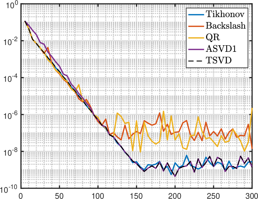
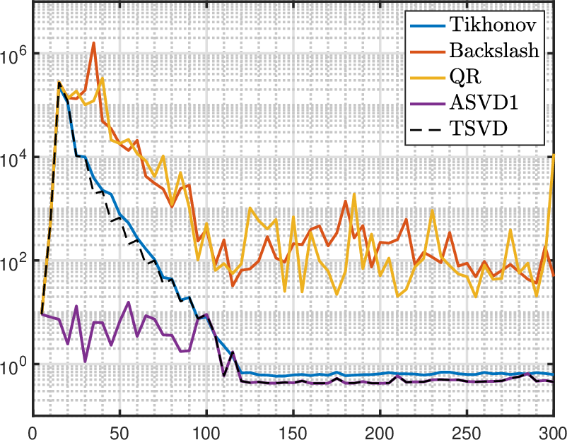
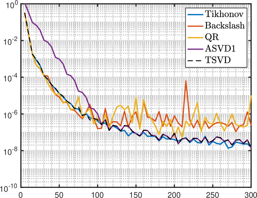
they may behave at worst like $1/\sqrt{\epsilon}$ before the onset of this asymptotic behaviour. Fig. 1 gives a typical example of this phenomenon. For the frame in question, the coefficient norm first increases exponentially fast, before decaying to $\mathcal{O}\left(1\right)$ in the limit. Notice that the approximation errors and coefficient norm obey the rough relationship described in (1.5): namely their ratio is approximately $\sqrt{\epsilon}$ for all $N$.

This phenomenon is not specific to the TSVD approximation. The same behaviour (in fact, sometimes somewhat worse) is seen for Tikhonov regularization, as well as QR factorization and Matlab’s backslash. See Fig. 2. It is interesting to note that in the limit $N\rightarrow\infty$ the TSVD and Tikhonov approximations (which are quite closely related) obtain both smaller errors and smaller coefficient values than QR or backslash.

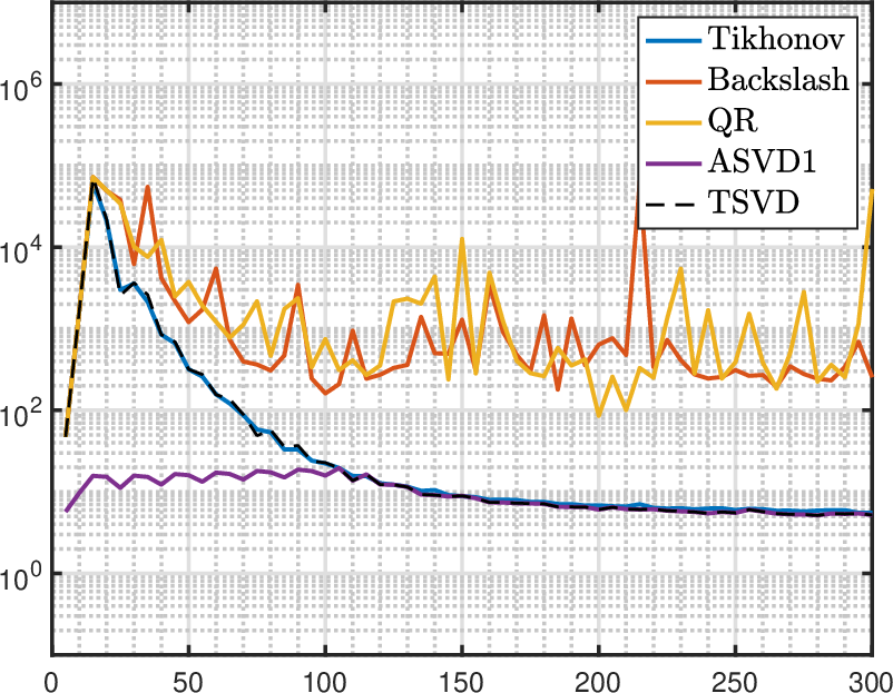This situation is bizarre. When $f$ is poorly approximated, i.e. $E_{N,\epsilon}(f)\gg\sqrt{\epsilon}$, the computed approximation has large coefficients. Yet when $f$ is well approximated, i.e. the error is close to $\sqrt{\epsilon}$, the approximation has small coefficients. Surely the approximation can be modified so that the coefficients remain small in the former regime? Given the redundancy of frames, there may be many ways to achieve such a relatively poor approximation without having to endure large coefficients.

In this paper, we solve this problem by modifying the TSVD approach. Rather than simply thresholding all singular values below the cutoff $\epsilon$, the idea is to adaptively choose the singular values based on the function being approximated. Specifically, we identify those singular values that are of insignificant importance in approximating $f$, but are responsible for growth of norm of the solution $\bm{x}$. In our first method, Adaptive SVD 1 (ASVD1), we discard a singular value $\sigma_{n}$ of the truncated Gram matrix $\bm{G}_{N}$ if either $\sigma_{n}\leq\epsilon$ or

$$\frac{\left|\left\langle\bm{y},\bm{v}_{n}\right\rangle\right|}{\sigma_{n}}>c{\left\|\bm{y}\right\|},$$

(1.7)

where $\bm{v}_{n}$ is the corresponding $n^{\text{th}}$ singular vector of $\bm{G}_{N}$ and $c>0$ is a parameter. Imposing constraints of the type (1.7) leads to regularized approximations for which coefficients are at worst of magnitude of $\mathcal{O}(\sqrt{N})$. While this bound is independent of the choice of the parameter $\epsilon$, it still depends on the degree of the approximation. Our second method, Adaptive SVD 2 (ASVD2), tackles this issue by imposing further regularization and leads to solutions whose norms are always bounded above by $c{\left\|\bm{y}\right\|}$. See §3 for further details of this method.

We analyze both schemes, ASVD1 and ASVD2, from the point of view of the approximation error and coefficient norm. For the ASVD1 approximation $\mathcal{A}^{\epsilon,c}_{N}f$ we show that

$$\|f-\mathcal{A}^{\epsilon,c}_{N}f\|\leq\|f-\mathcal{T}_{N}\bm{z}\|+\max\left\{\sqrt{\epsilon},\frac{\|f-\mathcal{T}_{N}\bm{z}\|}{c{\left\|\bm{y}\right\|}-\|\bm{z}\|}\right\}\|\bm{z}\|,\hskip 20.00003pt\forall\bm{z}\in\mathbb{C}^{N},\ {\left\|\bm{z}\right\|}<c{\left\|\bm{y}\right\|},$$

(1.8)

and if $\bm{x}^{\epsilon}=(x^{\epsilon}_{n})^{N}_{n=1}$ are the coefficients of $\mathcal{A}^{\epsilon,c}_{N}f=\sum^{N}_{n=1}x^{\epsilon}_{n}\phi_{n}$,

$${\left\|\bm{x}^{\epsilon}\right\|}\leq\min\left\{c\sqrt{BN}{\left\|f\right\|},E_{N,\epsilon}(f)/\sqrt{\epsilon}\right\}.$$

We also prove similar results for the ASVD2 scheme. At first glance, (1.8) may seem somewhat restrictive in comparison to the bound (1.3) for the TSVD approximation. Our analysis and numerical results show that this is not the case, provided $c$ is not too small. Indeed, since $\liminf_{N\rightarrow\infty}{\left\|\bm{y}\right\|}\geq\sqrt{A}{\left\|f\right\|}$, the bound (1.8) effectively states that the accuracy of the ASVD1 approximation is determined by how well $f$ can be approximated using coefficients $\bm{z}$ whose norm is at most $c\sqrt{A}$ times bigger than ${\left\|f\right\|}$. For the Legendre polynomial frame example (used in Figs. 1 and 2) we discuss how such coefficients arise in practice. We also examine the asymptotic behaviour of the schemes, and show that the ASVD1 and ASVD2 approximations behave like the TSVD approximation as $N\rightarrow\infty$. Our numerical examples show that ASVD1 and ASVD2 can often provide nearly as good approximations as TSVD without undergoing a regime of large coefficients. An example of this was already shown in Fig. 1.

The line of work [2, 1] on numerical frame approximation originated with the study of Fourier extensions [5], which are motivated by embedding methods for PDEs [13, 9, 4, 7, 14]. More recently, fast algorithms have been developed [10, 11, 12], as well as approaches suitable for higher-dimensional problems [1]. Frames are well-known tools in modern signal and image processing, coding theory and sampling theory. While they are less well-known in numerical analysis, there are numerous methods that rely on approximation systems that are nearly redundant. See [3] and references therein. Imposing the structure of a frame bestows problem with several pleasant properties. In particular, as discussed in §2, it guarantees the existence of at least one set of coefficients with small norm (the so-called frame coefficients). However, it is worth noting that the results in [3, 2] pertaining to the error and coefficient norm of the TSVD approximation do not require a frame structure.

The same is true for the corresponding results proved in this paper. Yet, by designing approximations with small-norm coefficients, we are implicitly assuming that the system admits such representations. This will not be the case in general redundant systems. For instance, the monomial basis $\phi_{n}(t)=t^{n-1}$ for, say, $L^{2}(0,1)$, is nearly redundant for large $N$, but most functions cannot be approximated using coefficients with small norm. Even within the frame setting, as we will see, if the constant $c$ is chosen too small, then ASVD1 and ASVD2 perform poorly. On the other hand, if the system is known to admit accurate, small-norm coefficient approximations and $c$ is chosen reasonably, then ASVD1 and ASVD2 are viable approaches. However, since the question of whether or not this holds is, in the absence of a frame, highly dependent on the system, we shall continue to work exclusively with frames in this paper.

Finally, we remark that one could consider alternatives to hard singular value thresholding as we do in this paper, for example, Tikhonov regularization (see Fig. 2) and the closely-related constrained least squares. However, thresholded SVDs are rather simpler to interpret and analyze, and it is not clear what benefits Tikhonov regularization might convey.

As observed, $\Phi$ is a frame if it satisfies the frame condition (1.1). If $A=B$, then $\Phi$ is a tight frame. Associated with any frame $\Phi$ is the synthesis operator

$$\mathcal{T}:\ell^{2}(I)\rightarrow\mathrm{H},\hskip 10.00002pt\bm{y}=\{y_{n}\}_{n\in I}\mapsto\sum_{n\in I}y_{n}\phi_{n}.$$

Its adjoint, the analysis operator, is given by

$$\mathcal{T}^{*}:\mathrm{H}\rightarrow\ell^{2}(I),\hskip 10.00002ptf\mapsto\{\langle f,\phi_{n}\rangle\}_{n\in I},$$

and the composition $\mathcal{S}=\mathcal{T}\mathcal{T}^{*}$, known as the frame operator, is

$$\mathcal{S}:\mathrm{H}\rightarrow\mathrm{H},\hskip 10.00002ptf\mapsto\sum_{n\in I}\langle f,\phi_{n}\rangle\phi_{n}.$$

The frame operator is self-adjoint, invertible, bounded and positive. If $\Phi$ is tight then $\mathcal{S}=A\mathcal{I}$.

A dual frame $\Psi=\{\psi_{n}\}_{n\in I}\subset\mathrm{H}$ of $\Phi$ is an indexed family that is frame for $\mathrm{H}$ and satisfies

$$f=\sum_{n\in I}\left\langle f,\psi_{n}\right\rangle\phi_{n}=\sum_{n\in I}\left\langle f,\phi_{n}\right\rangle\psi_{n},\hskip 10.00002pt\forall f\in\mathrm{H}.$$

(2.1)

The canonical dual frame is the frame $\Psi=\{\mathcal{S}^{-1}\phi_{n}\}_{n\in I}\subset\mathrm{H}$. For this frame, (2.1) gives

$$f=\sum_{n\in I}\left\langle f,\mathcal{S}^{-1}\phi_{n}\right\rangle\phi_{n}=\sum_{n\in I}\left\langle\mathcal{S}^{-1}f,\phi_{n}\right\rangle\phi_{n}.$$

(2.2)

The canonical dual frame has frame bounds $1/B$ and $1/A$, namely

$$1/B{\left\|f\right\|}^{2}\leq\sum_{n\in I}|\left\langle f,\mathcal{S}^{-1}\phi_{n}\right\rangle|^{2}\leq 1/A{\left\|f\right\|}^{2},\hskip 10.00002pt\forall f\in\mathrm{H}.$$

(2.3)

Notice that (2.2) gives $f=\sum_{n\in I}a_{n}\phi_{n}$, where $\bm{a}=\left\{\left\langle f,\mathcal{S}^{-1}\phi_{n}\right\rangle\right\}_{n\in I}$. These are the frame coefficients of $f$. They have minimal $\ell^{2}$-norm amongst all representations of $f$ in $\Phi$. In other words, if $f=\sum_{n\in I}a_{n}\phi_{n}=\sum_{n\in I}c_{n}\phi_{n}$ for some $\bm{c}=\left\{c_{n}\right\}_{n\in I}\in\ell^{2}(I)$, then ${\left\|\bm{c}\right\|}\geq{\left\|\bm{a}\right\|}$. These coefficients will play a role in our later analysis. However, we note in passing that approximating $f$ by $\sum_{n\in I_{N}}a_{n}\phi_{n}$, while it has the advantage of bounded coefficients, does not generally yield a good approximation for finite $N$ [3].

For each $N\in\mathbb{N}$, let $I_{N}\subset I$ be index sets satisfying $|I_{N}|=N$ and

$$I_{1}\subset I_{2}\subset\cdots,\hskip 20.00003pt\bigcup_{N=1}^{\infty}I_{N}=I.$$

Let $\Phi_{N}=\left\{\phi_{n}\right\}_{n\in I_{N}}$ be the finite set of frame elements with indices in $I_{N}$ and define the finite-dimensional subspace $\mathrm{H}_{N}=\mathrm{span}(\Phi_{N})$. Notice that $\Phi_{N}$ is a frame for $\mathrm{H}_{N}$. We let $\mathcal{T}_{N}:\mathbb{C}^{N}\rightarrow\mathrm{H}_{N}$, $\mathcal{T}^{*}_{N}:\mathrm{H}_{N}\rightarrow\mathbb{C}^{N}$, and $\mathcal{S}_{N}:\mathrm{H}_{N}\rightarrow\mathrm{H}_{N}$ denote the truncated synthesis, analysis and frame operators respectively.

We consider approximating an element $f\in\mathrm{H}$ from $\mathrm{H}_{N}$. Since $\mathrm{H}$ is a Hilbert space, the best approximation is the orthogonal projection onto $\mathrm{H}_{N}$. Write $\mathcal{P}_{N}:\mathrm{H}\rightarrow\mathrm{H}_{N}$ for the orthogonal projection operator. Using $\Phi_{N}$, we can write this projection as $\mathcal{P}_{N}f=\sum_{n\in I_{N}}x_{n}\phi_{n}=\mathcal{T}_{N}\bm{x}$, where the coefficients $\bm{x}=\{x_{n}\}_{n\in I_{N}}$ are a solution of the linear system

$$\bm{G}_{N}\bm{x}=\bm{y},\hskip 20.00003pt\bm{y}=\left\{\left\langle f,\phi_{n}\right\rangle\right\}_{n\in I_{N}},$$

(2.4)

where $\bm{G}_{N}=\{\langle\phi_{n},\phi_{m}\rangle\}_{m,n\in I_{N}}$ is the Gram matrix of $\Phi_{N}$. Since $\Phi_{N}$ may be linearly dependent, this linear system may be singular. In and of itself, this is of little consequence, since the projection $\mathcal{P}_{N}f$ itself is unique. However, even when $\Phi_{N}$ is linearly independent, $\bm{G}_{N}$ is ill-conditioned for large $N$ unless $\Phi$ happens to be a Riesz basis [3].

To deal with this ill-conditioning, [3, 2] used Truncated Singular Value Decompositions (TSVDs). Since $\bm{G}_{N}$ is nonnegative definite its singular values $\sigma_{n}$, $n\in I_{N}$, are its eigenvalues and its SVD takes the form $\bm{G}_{N}=\bm{V}\bm{\Sigma}\bm{V}^{*}$, where $\bm{V}\in\mathbb{C}^{N\times N}$ is unitary and $\bm{\Sigma}=\mathrm{diag}\left(\sigma_{n}\right)_{n\in I_{N}}$. Write $\{\bm{v}_{n}:n\in I_{N}\}$ for the columns of $\bm{V}$, which are left/right singular vectors of $\bm{G}_{N}$, i.e. $\bm{G}_{N}\bm{v}_{n}=\sigma_{n}\bm{v}_{n},n\in I_{N}$. Given a threshold $\epsilon>0$, define the regularized solution $\bm{x}^{\epsilon}$ of (2.4) as

$$\bm{x}^{\epsilon}=(\bm{G}^{\epsilon}_{N})^{{\dagger}}\bm{y},\hskip 20.00003pt\bm{G}^{\epsilon}_{N}=\bm{V}\bm{\Sigma}^{\epsilon}\bm{V}^{*},$$

where ${\dagger}$ denotes the pseudoinverse and $\bm{\Sigma}^{\epsilon}$ has $n^{\mathrm{th}}$ diagonal entry equal to $\sigma_{n}$ if $\sigma_{n}>\epsilon$ and zero otherwise. Applying $\mathcal{T}_{N}$, this gives rise to a regularized approximation, defined as

$$\mathcal{P}^{\epsilon}_{N}f=\mathcal{T}_{N}\bm{x}^{\epsilon}.$$

This approximation satisfies the bounds (1.3) and (1.4). In particular, the limiting accuracy is $\mathcal{O}(\sqrt{\epsilon})$. To attain $\mathcal{O}\left(\epsilon\right)$ accuracy, one can replace the square system (2.4), corresponding to a finite section [8], by a least-squares system $\bm{G}_{M,N}\bm{x}\approx\bm{y}$, where $\bm{G}_{M,N}=\{\langle\phi_{n},\phi_{m}\rangle\}_{m\in I_{M},n\in I_{N}}$ is the tall Gram matrix of size $M\times N$ (a so-called uneven section) and $\bm{y}=\{\langle f,\phi_{m}\rangle\}_{m\in I_{M}}$. As shown in [2], if $M$ is chosen sufficiently large in relation to $N$, one achieves $\mathcal{O}\left(\epsilon\right)$ accuracy in the limit $N\rightarrow\infty$.

This approach also addresses the case where it undesirable to compute $\bm{G}_{M,N}$ and $\bm{y}$ (typically their entries involve evaluating integrals). If $\bm{G}_{M,N}$ is replaced by the matrix $\bm{G}_{M,N}=\{\ell_{m,M}(\phi_{n})\}_{m\in J_{M},n\in I_{N}}\}$ and $\bm{y}$ by $\bm{y}=\{\ell_{m,M}(f)\}_{m\in J_{M}}$, where the $\ell_{m,M}$ are linear ‘measurement’ functionals – for example, pointwise samples – then the results of [2] guarantee $\mathcal{O}\left(\epsilon\right)$ accuracy in the limit under suitable conditions on the functionals $\ell_{m,M}$, $M$ and $N$.

In this paper, for our analysis we consider the simpler setup outlined above. However, we expect our theoretical results can be extended to setting of [2] with additional effort.

Before introducing our two main methods, we first define general thresholded SVD approximation. Let $\Lambda\subseteq I_{N}$ be a subset of singular values to be used in the approximation and $\bm{\Sigma}_{\Lambda}$ be the diagonal matrix with $n^{\text{th}}$ entry $\sigma_{n}$ if $n\in\Lambda$ and zero otherwise, and set

$$\bm{G}_{\Lambda}=\bm{V}\bm{\Sigma}_{\Lambda}\bm{V}^{*}.$$

(3.1)

Then we define the approximation

$$\mathcal{P}_{\Lambda}f=\mathcal{T}_{N}\bm{x}_{\Lambda},\hskip 20.00003pt\bm{x}^{\Lambda}=\left(\bm{G}_{\Lambda}\right)^{\dagger}\bm{y}=\bm{V}\left(\bm{\Sigma}_{\Lambda}\right)^{\dagger}\bm{V}^{*}\bm{y}.$$

Notice that the orthogonal projection $\mathcal{P}_{N}f$ and the TSVD approximation $\mathcal{P}^{\epsilon}_{N}f$ are special cases of $\mathcal{P}_{\Lambda}f$, corresponding to $\Lambda=I_{N}$ and $\Lambda=\Lambda^{\epsilon}=\{n\in I_{N}:\sigma_{n}>\epsilon\}$ respectively.

Since it will be useful later, we now show that $\mathcal{P}_{\Lambda}:\mathrm{H}\rightarrow\mathrm{H}$ is an orthogonal projection for any fixed $\Lambda$. First, to each singular vector $\bm{v}_{n}$ we associate an element $\xi_{n}\in\mathrm{H}_{N}$ defined by

$$\xi_{n}=\mathcal{T}_{N}\bm{v}_{n}=\sum_{m\in I_{N}}\left(\bm{v}_{n}\right)_{m}\phi_{m}.$$

Notice that the $\xi_{n}$ are orthogonal in $\mathrm{H}$ with

$$\langle\xi_{n},\xi_{m}\rangle=\langle\mathcal{T}_{N}\bm{v}_{n},\mathcal{T}_{N}\bm{v}_{m}\rangle=\langle\bm{v}_{n},\mathcal{T}_{N}^{*}\mathcal{T}_{N}\bm{v}_{m}\rangle=\sigma_{m}\langle\bm{v}_{n},\bm{v}_{m}\rangle=\sigma_{m}\delta_{n,m},$$

(3.2)

and hence form an orthogonal basis for $\mathrm{H}_{N}$. Next, notice that we may write

$$\bm{x}=\sum_{n\in I_{N}}\frac{\langle\bm{y},\bm{v}_{n}\rangle}{\sigma_{n}}\bm{v}_{n},\hskip 10.00002pt\bm{x}_{\Lambda}=\sum_{n\in\Lambda}\frac{\langle\bm{y},\bm{v}_{n}\rangle}{\sigma_{n}}\bm{v}_{n},$$

(3.3)

where $\langle\cdot,\cdot\rangle$ denotes the Euclidean inner product on $\mathbb{C}^{N}$, and $\langle\bm{y},\bm{v}_{n}\rangle=\sum_{m\in I_{N}}\langle f,\phi_{m}\rangle\overline{\left(\bm{v}_{n}\right)_{m}}=\langle f,\xi_{n}\rangle$. This gives

$$\mathcal{P}_{N}f=\mathcal{T}_{N}\bm{x}=\sum_{n\in I_{N}}\frac{\langle f,\xi_{n}\rangle}{\sigma_{n}}\xi_{n},\hskip 20.00003pt\mathcal{P}_{\Lambda}f=\mathcal{T}_{N}\bm{x}_{\Lambda}=\sum_{n\in\Lambda}\frac{\langle f,\xi_{n}\rangle}{\sigma_{n}}\xi_{n}.$$

(3.4)

From this, we deduce the claim. The operator $\mathcal{P}_{\Lambda}$ is precisely the orthogonal projection onto the subspace $\mathrm{H}_{\Lambda}=\mathrm{span}\{\xi_{n}:n\in\Lambda\}$.

For any fixed $\Lambda$, the expression (3.3) gives ${\left\|\bm{x}_{\Lambda}\right\|}^{2}=\sum_{n\in\Lambda}\frac{|\langle\bm{y},\bm{v}_{n}\rangle|^{2}}{\sigma^{2}_{n}}$. Since our goal is to maintain small-norm coefficients, this immediately leads to a possible strategy for choosing $\Lambda$: we simply exclude any $n$ for which the term $|\langle\bm{y},\bm{v}_{n}\rangle|/\sigma_{n}$ exceeds some tolerance. To determine a suitable tolerance, we recall (1.6). This motivates choosing the tolerance as a multiple of ${\left\|f\right\|}$. Of course, ${\left\|f\right\|}$ is generally unknown. However, notice that

$${\left\|\bm{y}\right\|}^{2}=\sum_{n\in I_{N}}|\langle f,\phi_{n}\rangle|^{2}\rightarrow\sum_{n\in I}|\langle f,\phi_{n}\rangle|^{2}\geq A{\left\|f\right\|}^{2},\hskip 20.00003ptN\rightarrow\infty,$$

where $\bm{y}$ is the right-hand side of the linear system (2.4). Hence, we take the tolerance to be some multiple of ${\left\|\bm{y}\right\|}$ instead. This leads to the following:

Notice that this definition of $\Lambda$ still retains the truncation of all small singular values below a threshold $\epsilon>0$. We will discuss the rationale for this in §4.

Due to the definition of $\Lambda$, ASVD1 leads to coefficients satisfying ${\left\|\bm{x}_{\Lambda}\right\|}\leq c\sqrt{N}{\left\|\bm{y}\right\|}\leq c\sqrt{B}\sqrt{N}{\left\|f\right\|},$ where the second inequality follows from the frame condition (1.1). Thus, the coefficients may not be truly bounded independently of $N$, although, as we show in Theorem 5.6, they will be $\mathcal{O}\left(1\right)$ in the limit $N\rightarrow\infty$. In our second method we avoid this behaviour:

Note that computing such a set $\Lambda$ is easily done by sorting the terms in the sum from smallest to largest. By definition, in this method we have ${\left\|\bm{x}_{\Lambda}\right\|}\leq c{\left\|\bm{y}\right\|}$. Since ${\left\|\bm{y}\right\|}\leq\sqrt{B}{\left\|f\right\|}$ due to (1.1), the coefficients are uniformly bounded in $N$.

In our first example, we consider an example of a general frame construction where an orthonormal basis is restricted to a subdomain. Such frames are particularly useful for approximating functions irregular-shaped domains, where finding orthonormal bases can be challenging [1]. For simplicity, we consider the one-dimensional case, where $\mathrm{H}=L^{2}(-1/2,1/2)$ is the space of square-integrable functions on the interval $(-1/2,1/2)$. Let

$$\psi_{n}(t)=\sqrt{n+1/2}P_{n}(t),\hskip 20.00003ptn\in I:=\mathbb{N}_{0},$$

be the orthonormal Legendre basis of $L^{2}(-1,1)$, where $P_{n}$ is the classical Legendre polynomial with normalization $P_{n}(1)=1$, and define $\phi_{n}=\psi_{n}|_{(-1/2,1/2)}$. The family $\{\phi_{n}\}^{\infty}_{n=0}$ forms a tight (in fact, Parseval) and overcomplete frame for $\mathrm{H}$ with frame bounds $A=B=1$.

Before showing numerical examples with this frame, we briefly discuss its approximation properties for smooth functions. Let $I_{N}=\{0,\ldots,N-1\}$ and $H^{k}(-1/2,1/2)$ be the standard Sobolev space of order $k\in\mathbb{N}$ with norm ${\left\|\cdot\right\|}_{H^{k}}$. Then, simplifying and slightly modifying the proof of [1, Thm. 5.2], one can show that if $f\in H^{k}(-1/2,1/2)$ then, for each $N$, there exists a vector of coefficients $\bm{z}\in\mathbb{C}^{N}$ such that

$${\left\|f-\mathcal{T}_{N}\bm{z}\right\|}\leq C_{k}N^{-k}{\left\|f\right\|}_{H^{k}},\hskip 20.00003pt{\left\|\bm{z}\right\|}\leq C_{k}{\left\|f\right\|}_{H^{k}},$$

(4.1)

where $C_{k}>0$ is a constant depending on $k$ only. Hence, the error term in (1.3) satisfies

$$E_{N,\epsilon}(f)\leq\min_{0\leq l\leq k}\left\{C_{l}(N^{-l}+\sqrt{\epsilon}){\left\|f\right\|}_{H^{l}}\right\}.$$

Therefore, for smooth functions $f$ TSVD approximation error is guaranteed decrease rapidly down to the level $\mathcal{O}\left(\sqrt{\epsilon}\right)$. An example of this behaviour was shown previously Fig. 1.

In Fig. 3 we compare ASVD1 and ASVD2 with TSVD for this frame, using various choices of $c$ and several different functions. As is evident, both ASVD methods successfully maintain small-norm coefficients, while yielding similar approximation errors to the TSVD approximation. Typically, the approximation error is slightly worse when $c$ is smaller, with the decline in performance depending on the function. The first fact is unsurprising: smaller $c$ means that coefficient vectors $\bm{z}$ with large norms but for which ${\|f-\mathcal{T}_{N}\bm{z}\|}$ is small are not attainable by the ASVD methods, whereas they may be obtained by TSVD. The dependence on the function is also unsurprising in light of (4.1). The function $f_{2}$ has large derivatives, and therefore the coefficient vectors of (4.1) have norms growing rapidly with the Sobolev order $k$. When $c$ is small, they may not be realizable by the ASVD approximations. Conversely, the derivatives of $f_{1}$ grow more slowly, meaning such coefficient vectors are potentially realizable.

In Fig. 4 we examine the influence of $c$ further. Notice that when $c$ is too small – specifically, less than one for ASVD1 and less than two for ASVD2 – the error behaves badly, either converging very slowly, or jumping from small to large. In §5, we will support these conclusions with theory: specifically, we show that $c>1/A$ and $c>2/A$ respectively are sufficient for convergence, where $A$ is the lower frame bound (recall that $A=1$ for the Legendre polynomial frame). See Theorem 5.6.

Finally, in Fig. 5 we examine why a truncation parameter $\epsilon>0$ is generally a good idea in ASVD1 and ASVD2. This figure shows the behaviour of each method when no truncation occurs, i.e. $\epsilon=0$. Notice that for ASVD1 the method still produces an acceptable error. Yet the coefficients are no longer $\mathcal{O}\left(1\right)$ in the limit $N\rightarrow\infty$, unlike those of the TSVD approximation. Indeed, the limiting accuracy and coefficient norm both appear to scale with $c$. This is undesirable; we would certainly prefer the ASVD methods to retain the desirable limiting behaviour of the TSVD approximation. For ASVD2 the behaviour is even worse. For smaller $c$, the error jumps to $\mathcal{O}\left(1\right)$, indicating lack of (or at best very slow) convergence of the approximation. Incorporating a threshold appears vital for rapid convergence in this case. Our theoretical results in §5 support this conclusion.

We now consider approximating functions of the form

$$f(t)=w(t)g(t)+h(t),\hskip 10.00002ptt\in[0,1],$$

(4.2)

where $g$ and $h$ are smooth functions, and $w\in\mathrm{L}^{2}(0,1)$ is a known function that may be singular. We shall consider the case $w(t)=\log(t)$, i.e. $f(t)$ has a logarithmic singularity at $t=0$. This problem was considered in [2], and the approach used therein is employs the frame

$$\Phi=\{\varphi_{n}\}^{\infty}_{n=0}\cup\{\psi_{j}\}^{K-1}_{j=0},$$

(4.3)

where $\varphi_{n}$ is the orthonormal Legendre polynomial basis on $(0,1)$, $\psi_{j}(t)=\log(t)\varphi_{j}(t)$ and $K\in\mathbb{N}$. This forms a frame for any finite $K$. It is an example of a general construction of a frame, in which an orthonormal basis of a Hilbert space $\mathrm{H}$ is augmented with a finite number of arbitrary elements from $\mathrm{H}$. The rationale for using (4.3) for functions of the form (4.2) that the $\psi_{j}$ capture the logarithmic singularity up to some finite order depending on $K$ and the polynomials capture the remaining smooth part. To see this, let

$$\Phi_{N}=\{\psi_{j}\}^{K-1}_{j=0}\cup\{\varphi_{n}\}^{N-K-1}_{n=0},\hskip 20.00003ptN>K,$$

Similar to the previous example, we can show that exists an approximation to $f$ from $\Phi_{N}$ with bounded coefficients that converges at an algebraic rate depending on $K$. Let $p=\sum^{K-1}_{k=0}z_{k}\varphi_{k}$ be the $K^{\mathrm{th}}$ order Taylor polynomial of $g$ around $t=0$, so that $p^{(j)}(0)=g^{(j)}(0)$ for $j=0,\ldots,K-1$. Then let

$$q=\mathcal{Q}_{N-K}(h+w(g-p))=\sum^{N-K-1}_{n=0}z_{K+n}\varphi_{n},\hskip 20.00003ptz_{K+n}=\langle h+w(g-p),\varphi_{n}\rangle,$$

be the orthogonal projection of $h+w(g-p)$ onto $\mathrm{span}\{\varphi_{n}\}^{N-K-1}_{n=0}$. Clearly,

$$|z_{j}|\leq C_{K}\max_{0\leq l<K}|g^{(l)}(0)|\leq C_{K}{\left\|g\right\|}_{H^{K}},\hskip 20.00003ptj=0,\ldots,K-1,$$

for some constant $C_{K}>0$ depending on $K$. This implies that the coefficients $\bm{z}=(z_{n})^{N-1}_{n=0}$ are uniformly bounded in $N$. Indeed, we have

$$\sqrt{\sum^{N-K-1}_{n=0}|z_{K+n}|^{2}}\leq{\left\|h+w(g-p)\right\|}\leq{\left\|h\right\|}+{\left\|w(g-p)\right\|}\leq{\left\|h\right\|}+C_{K}{\left\|g\right\|}_{H^{K}},$$

where $C_{K}$ is a possibly different constant, and therefore

$${\left\|\bm{z}\right\|}\leq{\left\|h\right\|}+C_{K}{\left\|g\right\|}_{H^{K}}.$$

Moreover, the approximation $\mathcal{T}_{N}\bm{z}$ converges algebraically fast to $f$. To see why, observe that, by construction

$${\left\|f-\mathcal{T}_{N}\bm{z}\right\|}={\left\|w(g-p)+h-\mathcal{Q}_{N-K}(w(g-p)+h)\right\|}.$$

Since $h$ is smooth by assumption and $g-p$ vanishes along with its first $K-1$ derivatives at $t=0$, the function $w(g-p)+h$ has roughly $K$ orders of smoothness. Hence ${\left\|f-\mathcal{T}_{N}\bm{z}\right\|}$ decays at an algebraic rate in $N$ depending on $K$.

Having provided the rationale for using this frame, we now present numerical results. Rather than solving (2.4), we consider the setup of [2] (see Remark 2.3) and compute an approximation in $\mathrm{H}_{N}$ using the data

$$\bm{y}=\{f(t_{m,M})\}^{M}_{m=1},\hskip 20.00003ptt_{m,M}=\frac{\cos(\frac{2m-1}{2M}\pi)+1}{2},\hskip 20.00003ptm=1,\ldots,M.$$

(4.4)

Note that the points $t_{m,M}$ are Chebyshev nodes in $(0,1)$. To do this, we simply modify the TSVD, ASVD1 and ASVD2 methods to approximately solve the least-squares problem

$$\bm{G}_{M,N}\bm{z}\approx\bm{y},\hskip 20.00003pt\bm{G}_{M,N}=\left\{\phi_{n}(t_{m,M})\right\}^{M,N-1}_{m=1,n=0}\in\mathbb{C}^{M\times N},$$

(4.5)

In Fig. 6 we compare these methods for this problem with the oversampling $M/N=2$.

This experiment reveals several interesting phenomena. First, when $c$ is small, the convergence of ASVD1 and ASVD2 suffers, in particular when $\alpha\gg 1$ is larger. This is as expected. For the function considered, the $K^{\mathrm{th}}$ derivative of $g(t)=\log(t)\cos(\alpha t)$ scales like $\alpha^{K}$. When $\alpha$ is large, the coefficients constructed above might not be attainable by ASVD1 or ASVD2. The slower rates of convergence shown in the figure support this argument. Second, for small $N$, ASVD1 and ASVD2 actually achieve slightly smaller errors than TSVD. Informally, this might be explained as follows: by constraining the singular values, we prohibit larger-norm solutions, which asymptotically might give the optimal rate of convergence, but are associated with larger constants in the error bounds.

We commence with the error bounds:

This result explains the effect of constraining ${\|\bm{x}^{\Lambda}\|}$. While (5.1) allows for arbitrary coefficients $\bm{z}$, in (5.2) and (5.3) the error is controlled only by those $\bm{z}$ that satisfy a certain bound. It is notable that the bound on $\bm{z}$ for ASVD2 is much stricter than it is for ASVD1. We discuss further consequences of Theorem 5.1 in a moment. First, we consider the coefficient norms:

This agrees with the numerical results. The coefficients $\bm{x}^{\Lambda}$ of ASVD1 or ASVD2 remain bounded (or nearly bounded) in the pre-asymptotic regime, and then match the coefficient bound for TSVD asymptotically as $N\rightarrow\infty$.

We now give further insight into Theorem 5.1. To do so, we define the following:

Notice that if we replace the maximum by a sum, then the ASVD1 error (5.8) can be replaced by the simpler expression

$${\left\|f-\mathcal{P}_{\Lambda}f\right\|}\leq\left(\frac{c(1-\delta)}{c(1-\delta)-a^{2}}\delta+a\sqrt{\epsilon}\right){\left\|f\right\|},\hskip 20.00003pt\forall c>\frac{a^{2}}{1-\delta}.$$

Hence this theorem shows that whenever there is sequence of coefficients $\bm{z}$ approximating $f$ to a relative error of $\delta$, and which do not grow too large (depending on $c$), then TSVD and ASVD1 are guaranteed the same error bound up to a constant depending on $c$, $\delta$ and $a$. Larger $c$ allows means this holds for bigger $a$, thus, as expected, making it easier in some sense to achieve an error of size $\delta$. Notice that for ASVD2 this result only applies when $\delta=\mathcal{O}\left(\sqrt{\epsilon}\right)$. This is due to the condition on $\bm{z}$ in Theorem 5.1, and suggests that ensuring fast error decay with ASVD2 may be more challenging, especially for smaller $c$.

It is informative to examine this result for the Legendre polynomial frame of §4.1 . Recall that (4.1) asserts the existence of bounded coefficients yielding algebraic rates of convergence. Setting $\delta=D_{k,f}N^{-k}$, where $D_{k,f}=C_{k}{\left\|f\right\|}_{H^{k}}/{\left\|f\right\|}_{L^{2}}$ and $a=D_{k,f}$, it follows that

$${\left\|f-\mathcal{P}_{\Lambda}f\right\|}\leq\left(N^{-k}+\sqrt{\epsilon}\right)D_{k,f}{\left\|f\right\|},$$

for TSVD. For ASVD1, if $N\geq(2D_{k,f})^{1/k}$ (the factor of $2$ is arbitrary), we have

$${\left\|f-\mathcal{P}_{\Lambda}f\right\|}\leq\left(\frac{c}{c-2D^{2}_{k,f}}N^{-k}+\sqrt{\epsilon}\right)D_{k,f}{\left\|f\right\|},\hskip 20.00003ptc>2D^{2}_{k,f},$$

This agrees with the numerical examples. For sufficiently large $c$, we expect little or no deterioration in the rate of error decay. But for small $c$, in particular, when ${\left\|f\right\|}_{H^{k}}$ grows rapidly with $k$, we may see slower decay due to unattainability in ASVD1 of the coefficient vectors giving the faster algebraic rates.

References

- [1] B. Adcock and D. Huybrechs. Approximating smooth, multivariate functions on irregular domains. arXiv:1802.00602, 2018.
- [2] B. Adcock and D. Huybrechs. Frames and numerical approximation II: generalized sampling. arXiv:1802.01950, 2018.
- [3] B. Adcock and D. Huybrechs. Frames and numerical approximation. SIAM Rev., 61(3):443–473, 2019.
- [4] D. Boffi, N. Cavallini, and L. Gastaldi. The finite element immersed boundary method with distributed Lagrange multiplier. SIAM J. Numer. Anal., 53(6):2584–2604, 2015.
- [5] J. Boyd. Fourier embedded domain methods: extending a function defined on an irregular region to a rectangle so that the extension is spatially periodic and . Appl. Math. Comput., 161(2):591–597, 2005.
- [6] O. Christensen. An Introduction to Frames and Riesz Bases. Applied and Numerical Harmonic Analysis. Birkhäuser, 2nd edition, 2016.
- [7] F. Kasolis, E. Wadbro, and M. Berggren. Analysis of fictitious domain approximations of hard scatterers. SIAM J. Numer. Anal., 2015(5):2347–2362, 2015.
- [8] M. Lindner. Infinite Matrices and their Finite Sections. Frontiers in Mathematics. Birkhäuser Verlag, Basel, 2006.
- [9] S. H. Lui. Spectral domain embedding for elliptic PDEs in complex domains. J. Comput. Appl. Math., 225(2):541–557, 2009.
- [10] M. Lyon. A fast algorithm for Fourier continuation. SIAM J. Sci. Comput., 33(6):3241–3260, 2012.
- [11] R. Matthysen and D. Huybrechs. Fast algorithms for the computation of Fourier extensions of arbitrary length. SIAM J. Sci. Comput., 38(2):A899–A922, 2016.
- [12] R. Matthysen and D. Huybrechs. Function approximation on arbitrary domains using Fourier extension frames. SIAM J. Numer. Anal., 56(3):1360–1385, 2018.
- [13] R. Pasquetti and M. Elghaoui. A spectral embedding method applied to the advection–diffusion equation. J. Comput. Phys., 125:464–476, 1996.
- [14] D. Shirokoff and J.-C. Nave. A sharp-interface active penalty method for the incompressible Navier–Stokes equations. J. Sci. Comput., 62(1):53–77, 2015.