Devanshu Agrawal, Theodore Papamarkou, Jacob Hinkle
Wide Neural Networks with Bottlenecks are Deep Gaussian Processes
Abstract
There has recently been much work on the “wide limit” of neural networks, where Bayesian neural networks (BNNs) are shown to converge to a Gaussian process (GP) as all hidden layers are sent to infinite width. However, these results do not apply to architectures that require one or more of the hidden layers to remain narrow. In this paper, we consider the wide limit of BNNs where some hidden layers, called “bottlenecks”, are held at finite width. The result is a composition of GPs that we term a “bottleneck neural network Gaussian process” (bottleneck NNGP). Although intuitive, the subtlety of the proof is in showing that the wide limit of a composition of networks is in fact the composition of the limiting GPs. We also analyze theoretically a single-bottleneck NNGP, finding that the bottleneck induces dependence between the outputs of a multi-output network that persists through extreme post-bottleneck depths, and prevents the kernel of the network from losing discriminative power at extreme post-bottleneck depths.
keywords
Bayesian neural networks, deep learning, Gaussian processes, kernels, phase transitions1 Introduction
Deep neural networks have found great empirical success, achieving state-of-the-art performance on a variety of tasks such as those in computer vision and natural language understanding (Krizhevsky et al. 2012; Antipov et al. 2015; Liang et al. 2017). There is considerable interest in understanding the theoretical aspects of deep neural networks both to establish guarantees on the behavior of these models on certain classes of problems as well as to guide architecture design and optimization. One avenue of pursuit in this endeavor leads to the study of Bayesian neural networks (BNNs), where the parameters of the network are random variables following some probability distributions. BNNs thus bring the formalism and machinery of probability theory to bear on neural networks.
It is a foundational result that a BNN converges to a Gaussian process (GP) in the “wide limit”—i.e., as the widths of all hidden layers are sent to infinity while the prior distributions on weights are sharpened accordingly (Neal 1996). The resulting GP is called a “neural network Gaussian process” (NNGP). Although NNGP limits have been derived from various BNN architectures, they cannot be obtained from architectures requiring some hidden layers to remain narrow, such as certain autoencoders. It seems intuitive that the wide limit of a BNN with some hidden layers restricted to finite-width “bottlenecks” is a composition of NNGPs, but until now this claim has not been proven. Such a composition of GPs is called a “deep Gaussian process” (DGP) in the literature (Damianou and Lawrence 2013). Although DGPs were inspired by the compositional structure of deep neural networks, their connection to BNNs has not been established formally.
In this paper, we give a formal proof of the convergence of BNNs with bottleneck layers to a DGP in the wide limit, where the DGP is a composition of NNGPs. In doing so, we unify the two major approaches to making GPs “deeper”—NNGPs and DGPs, thus allowing NNGPs to be examined in the DGP framework. We will refer to the limiting DGP as a “bottleneck NNGP”. Even though the result is intuitive, the proof is nontrivial as it requires us to formally justify that the limit of a composition of BNNs equals the composition of the limiting NNGPs.
In the bottleneck NNGP limit, we consider a sequence of BNNs all having the same architecture except that some hidden layers are growing to infinite width (Fig. 1). We call the hidden layers held to finite widths “bottleneck layers” or simply “bottlenecks”, and we call each network in the sequence a “bottleneck BNN”. We use the term “component” to refer to any subnetwork that is either (1) between the input layer and the first bottleneck layer, (2) between two bottleneck layers with no bottlenecks in between, or (3) between the last bottleneck layer and the output layer; each BNN is thus a composition of components, and each component maintains constant input and output dimensions with only its hidden layers growing in width over the sequence of networks.
We know that each sequence of corresponding components converges to an NNGP in the wide limit. It is therefore intuitive to expect that the sequence of bottleneck BNNs (each BNN being a composition of components) converges to the composition of NNGPs—i.e., a bottleneck NNGP. However, this fact is not immediate, and care must be taken to verify that the limit procedure can be exchanged with the composition of components. In particular, we find that this exchangeability holds if each post-bottleneck component converges to an NNGP with a sufficient amount of uniformity with respect to its inputs.
We demonstrate the utility of bottleneck NNGPs and their link to no-bottleneck NNGPs empirically, showing that restricting a hidden layer of an NNGP to a bottleneck can boost its model likelihood on three example datasets11 1 Code for our simulations and experiments is available at https://code.ornl.gov/d0a/bottleneck_nngp. .
We also characterize the effect of a bottleneck layer theoretically by analyzing an example multi-output single-bottleneck NNGP with rectified linear unit (ReLU) activation. We find that the bottleneck induces dependence between distinct response variables and derive a closed-form expression for the correlation between the squares (i.e., quadratic correlation) of the response variables. We show that in the deep post-bottleneck limit (infinitely many infinite-width hidden layers after the bottleneck), the quadratic correlation tends to when the network is in the “disordered phase”—so that response variables decouple—but remains a nontrivial function of the inputs in the “ordered phase”—so that information about the inputs can be recovered. We identify the prior variance of the network weights as the order parameter responsible for the phase transition.
Similarly, in the deep post-bottleneck limit, we obtain a closed-form expression for the quadratic correlation of outputs of a single response variable given two inputs. We find that the quadratic correlation is 100% in the “disordered phase”—so that the network has lost all discriminative power at infinite depth—but is surprisingly a nontrivial function of the inputs in the “ordered phase”. This behavior in the ordered phase stands in stark contrast to that of no-bottleneck NNGPs and indicates that bottleneck layers are essential for a very deep network to maintain discriminative power.
2 Preliminaries
In this section, we review prior work on DGPs and NNGPs to contextualize and motivate the bottleneck NNGP model. We also review the main theorem of 17 in Sec. 2.3, introducing notation that will be essential to stating our main result in Sec. 3.1.
2.1 Deep Gaussian processes
Compositions of GPs are known as deep Gaussian processes (DGPs) in the literature and were originally motivated by the success of deep neural networks and the hope to obtain similar success on small data sets where Bayesian methods generally shine (Damianou and Lawrence 2013). DGPs have indeed been shown to outperform shallow GPs on a variety of regression and classification tasks (Damianou and Lawrence 2013; Salimbeni and Deisenroth 2017). Damianou and Lawrence 2013 implement DGPs in a sparse variational inducing points framework based on the work of Titsias 2009 in order to simplify the composition of GPs to a set of separate but coupled GPs, but their implementation is restricted to small data sets with only a few hundred entries. Much of the DGP literature has therefore been dedicated to developing more efficient and scalable implementations (Hensman and Lawrence 2014; Dai et al. 2015; Bui et al. 2016; Wang et al. 2016; Salimbeni and Deisenroth 2017). Salimbeni and Deisenroth 2017 in particular show that DGPs can be put into a stochastic variational framework as in Hensman et al. 2013, allowing the models to be applied to much larger data sets.
DGPs offer the additional advantage that they can capture correlation between multiple outputs (Wang et al. 2016). In contrast, the outputs of a shallow multi-output GP are by default independent, which can limit predictive performance for multi-output problems. Although methods have been proposed to model correlation in a shallow multi-output GP, such as through linear mixing of latent outputs (Bonilla et al. 2008; Alvarez and Lawrence 2009), DGPs capture correlation naturally through shared feature representations in the latent “bottleneck space”—similar to the approach taken with multi-task deep neural networks (Ruder 2017). DGPs have therefore been applied to problems that can benefit from modeling correlation between multiple outputs, such as multi-task regression (Alaa and van der Schaar 2017) and tasks involving partially observed multivariate outputs—i.e., missing values (Wang et al. 2016).
The mechanism by which the outputs of a DGP are made dependent predates the DGP model itself, as it was first introduced in the context of the Bayesian Gaussian process latent variable model (GP-LVM), where a Gaussian prior is placed on the latent inputs of a GP (Lawrence 2004; Titsias and Lawrence 2010); for regression, each input is concatenated with such a latent random variable before it is fed into the GP (Dutordoir et al. 2018). The outputs then become dependent through their dependence on the common set of latent random variable inputs, which are analogous to the bottleneck activations of a DGP. However, it still remains quantitatively unclear how the introduction of a bottleneck layer—or in the case of an NNGP, the restriction of a layer to finite width—induces correlation between multiple outputs under the prior and how this translates to correlation under the posterior. Moreover, although this mechanism is well-established for the GP-LVM and DGP models, it is conspicuously absent in the NNGP literature and thus its implications for NNGPs are not fully understood.
The DGP prior has been studied by Lu et al. 2019, who show that for a single-bottleneck DGP with a single response variable, the prior has heavy tails, in contrast to shallow GPs. Their calculation of the prior kurtosis is similar to that of the quadratic correlation between distinct response variables of a multi-output DGP, but this connection is not discussed. Moreover, they only consider a bottleneck of width one and primarily focus on stationary kernels that do not arise from NNGP limits with common activation functions.
There is considerable interest in understanding the “deep limit” of DGPs—i.e. when arbitrarily many GPs are composed together. Duvenaud et al. 2014 and Dunlop et al. 2018 show that DGPs with a certain class of kernels have trivial, pathological, or convergent deep limits, meaning that increasing the depth of a DGP beyond some point is either detrimental to performance or diminishingly beneficial. However, they do not consider NNGP kernels and thus do not analyze deep limits of architectures with both bottlenecks and infinitely many infinite-width hidden layers.
Although DGPs were inspired by deep neural networks, there is little literature concretely establishing their connection. Duvenaud et al. 2014 discuss the connection between DGPs and neural networks at a high level to motivate studying the deep limit of DGPs with radial basis function (RBF) kernels, but the implication for neural networks is not treated formally. Gal and Ghahramani 2015 consider a DGP where the kernel of each GP layer is an integral as in Williams 1997. They show that a Monte Carlo estimation of the kernels leads to a BNN approximation of the DGP, where the width of a hidden layer corresponds to the size of the Monte Carlo sample. However, they do not formally verify convergence of a BNN to a DGP in the limit of infinite width. Moreover, their bottleneck layers have no activation function and are not scaled to allow an NNGP to be recovered as the bottlenecks are sent to infinite width.
2.2 Wide neural networks as GPs
A foundational result in the study of BNNs came when Neal 1996 showed that a BNN with one hidden layer converges to a GP in the “wide limit”—i.e., as the number of hidden neurons is sent to infinity. Shortly after, Williams 1997 derived analytic expressions for the kernel of the GPs corresponding to neural networks with sigmoidal and Gaussian hidden units. These works connected neural networks to the world of Bayesian nonparametrics and kernel methods and thus offered a new perspective to interrogate and probe the behavior of neural networks. In particular, while training neural networks is challenging since it requires the optimization of highly non-convex objective functions, GPs are nonparametric models that admit exact Bayesian inference, where the predictive posterior distribution can be written in closed form (Rasmussen and Williams 2006).
Since the works of Neal 1996; Williams 1997, new insights into BNNs have steadily emerged. Cho and Saul 2009 interpreted a BNN as a feature embedding map and derived the equations for the propagation of a kernel through the layers of a deep neural network with rectified polynomial unit activations. Subsequent works built upon these findings to elucidate key theoretical aspects of neural networks including expressivity (Poole et al. 2016), generalization power (Hazan and Jaakkola 2015), initialization (Daniely et al. 2016), and trainability (Schoenholz et al. 2016). More recently, the original result by Neal 1996 has been extended to deep architectures by showing that a deep BNN converges to a GP as the widths of all hidden layers are simultaneously sent to infinity (35; 17). We refer to GPs that arise from such a limit as “neural network Gaussian processes” (NNGPs). As the work of 17 illustrates, this extension is nontrivial; the proof by Neal 1996 relies on the Central Limit Theorem, but the assumption of independent and identically distributed (IID) random variables necessary for the Central Limit Theorem does not hold for deep architectures. The proof by 17 for deep architectures is instead based on a more exotic central limit theorem as given in Blum et al. 1958.
Since the extension of the NNGP limit to deep architectures, there have been a number of works establishing and analyzing analogous wide-limit results for more modern neural network architectures that are used in practice today. These include convolutional neural networks (Garriga-Alonso et al. 2019; Novak et al. 2019), weight-tied autoencoders (Li and Nguyen 2019), and most generally any network that can be represented as a “tensor program”—including recurrent neural networks and attention networks among others (Yang 2019). Alongside these works, new insights into the trainability and generalization power of neural networks have continued to emerge, based on the tractable learning dynamics of neural networks in the wide limit (Jacot et al. 2018; Lee et al. 2019; Arora et al. 2019).
One application of the NNGP limit that is of particular note is that it can make the analysis of the “deep limit”—i.e., as the number of hidden layers is sent to infinity—tractable (Poole et al. 2016; Schoenholz et al. 2016; Yang and Schoenholz 2017; Lee et al. 2017). Poole et al. 2016 and Schoenholz et al. 2016 show that the correlation between two inputs transformed through an NNGP with sigmoidal activation function has a fixed point at 100% in the deep limit that transitions from stable to unstable (i.e., ordered to chaotic) when the variances of the Gaussian weights and biases cross a certain phase boundary; the network is shown to be highly expressive in the chaotic phase and optimally trainable near the phase boundary. In contrast, for networks with rectified linear unit (ReLU) activations, the correlation between transformed inputs has a stable fixed point at 100% regardless of the weight variance, implying that an NNGP with ReLU activation has no discriminative power at infinite depth (Lee et al. 2017).
The works described above all consider BNNs in the wide limit, and thus the results and insights therein do not apply to neural network architectures that require one or more finite width or “bottleneck” layers. One of the most important classes of neural networks that frequently require bottleneck layers is that of autoencoders (Hinton and Salakhutdinov 2006; Kingma and Welling 2014). Another example is neural networks with a word embedding layer, which is currently key to the successful application of neural networks to natural language understanding (Mikolov et al. 2013). Both word embedding layers and many autoencoder models aim to find dense feature representations and therefore depend on low-dimensional spaces. Even for neural network architectures that are not directly meant for dense representation learning, it has still been argued and demonstrated that bottleneck layers perform data compression and therefore help to boost generalization power (Tishby and Zaslavsky 2015). Particularly for fully-connected architectures, which is what we consider in this work, it has been shown that the insertion of linear bottleneck layers between two linear ReLU layers boosts predictive performance by reducing sparsity and improving gradient flow (Lin et al. 2015). This prompts the question: How can insights based on very wide BNNs be generalized to networks in which one or more hidden layers are held fixed to a finite width? The first step in addressing this question is to understand what happens if we let all but finitely many hidden layers of a BNN grow to infinite width. We call these finite-width hidden layers “bottleneck layers”. It is already established that the component networks between consecutive bottleneck layers converge to GPs, and thus we intuitively expect a BNN with bottleneck layers to converge in the wide limit to a composition of GPs. In Sec. 3.1, we formally verify that this is the case.
2.3 The no-bottleneck NNGP limit
The bottleneck NNGP limit is a generalization of the (no-bottleneck) NNGP result proved by 17. Moreover, one component of our proof is verifying that BNNs converge in distribution uniformly on compact sets, and our approach to proving this closely follows the proof of 17. In this section, we state the NNGP limit result by 17, which also allows us to introduce key concepts and notation along the way.
We consider a traditional fully-connected network mapping to with hidden layers and nonlinearity . Let be the width of the -th hidden layer. The propagation of an input through the network is then governed by a recursion with initial step
| (1) |
and for ,
| (2) | ||||
| (3) |
In Eq. (2), ranges from to . In Eq. (3), ranges from to for , and from to for . We refer to and the as the preactivations into and activations out of the -th hidden layer, respectively. The top-most preactivations are the outputs of the network.
We require mild assumptions on the nonlinearity for our main theorem to hold; these are the same assumptions made by 17, namely the linear envelope condition.
Definition 1 (Linear envelope condition).
A nonlinearity is said to satisfy the linear envelope condition if it is continuous and there exist positive constants and such that
Many popular activation functions such as tanh, ReLU, and leaky ReLU satisfy the linear envelope condition, and thus our result is quite general with regards to the choice of nonlinearity.
We now turn the above network into a random network by placing IID normal distributions on the weights and biases of the network:
| (4) | ||||
| (5) |
where we set for the purpose of defining these distributions. The variance of the weights after the first layer are scaled inversely to the preceding hidden layer width so that the Central Limit Theorem can be applied to the convergence of BNNs to a GP. With a slight abuse of terminology, we will call the constants and “weight and bias variance hyperparameters” even though is not the actual variance of the weights.
The output is now a random vector of dimension for each input , and we therefore understand a BNN as an instance of a stochastic process. We give a formal definition next, after we introduce some notation. If is a probability space and is a measurable space, then an -valued stochastic process with index set is a function such that is a measurable function for each . By the notation , we refer to the random variable defined by .
Definition 2 (Bayesian neural network).
17 prove the following theorem concerning the convergence of BNNs with no bottleneck layers.
Theorem 3 (NNGP theorem, 17).
Let be a sequence of BNNs mapping to each with hidden layers of widths , , and nonlinearity that satisfies the linear envelope condition. If is strictly increasing in for each , then restricted to a countable index set converges in distribution to the Gaussian process , where is a kernel defined recursively by Eqs. (6)-(7).
Note that we use the suffix instead of a subscript to index a sequence of stochastic processes. Convergence in distribution is defined in the measurable space of -valued sequences; details are provided in Appendix A. The limiting GP in Thm. 3 is called a neural network Gaussian process (NNGP). If is the limiting NNGP of , then the NNGP kernel is defined through a recursion with initial step
| (6) |
and for ,
| (7) |
where is the matrix with entries ; here we could have used in place of for any since the NNGP preactivations into the -th hidden layer are IID over . The (countably infinite) kernel matrix is therefore block-diagonal with the -th block .
The kernel in Thm. 3 is given by . Observe that the outputs of the BNNs converge to IID GPs so that all correlations between the outputs of the networks are lost in the infinite width limit. We will see that bottleneck layers help to preserve some correlations between outputs.
3 The bottleneck NNGP theorem
In this section, we state and prove the bottleneck NNGP theorem, we show that a single-bottleneck NNGP approximates a no-bottleneck NNGP as the bottleneck width is increased, and we explore the effect of depth and width on bottleneck NNGPs using three example datasets.
3.1 Statement of main theorem
We now state our main theorem, which is a direct generalization of Thm. 3 to compositions of BNNs. Given two stochastic processes and , we define the composition as the stochastic process with
Theorem 4 (Bottleneck NNGP theorem).
Let for with and . For each , let be a sequence of BNNs mapping to with hidden layers of widths , , and nonlinearity that satisfies the linear envelope condition. If is strictly increasing in for each and , then the sequence of bottleneck random neural networks restricted to a countable index set converges in distribution in to , where is the limiting NNGP of .
Remark 5 (Nonlinear bottleneck).
Theorem 4 as stated above assumes no nonlinearity on the bottleneck layers. However, the theorem also holds when we replace and with and respectively for , that is when we scale the weights after each bottleneck layer by layer width in the same way as all other weights after a hidden layer and and we place nonlinearities on the bottleneck layers. The proof is nearly identical to the proof of Thm. 4 (see Remark 28 in Appendix B.2 for details).
Remark 6 (Discontinuous nonlinearity).
Theorem 4 holds even if the nonlinearity is continuous only almost everywhere, as long as is continuous at or . Each of these two conditions ensures that the Continuous Mapping Theorem is still applicable in Lemmas 31-33 (see Remark 29 in Appendix B.2 for details). This extends the class of allowable nonlinearities to include such prominent examples as the Heaviside step function used in the first perceptron model (Rosenblat 1958).
Remark 7 (Converse of the main theorem).
The converse of Thm. 4—that every DGP is the bottleneck NNGP limit of a BNN with IID priors and a nonlinearity satisfying the linear envelope condition—does not hold. A simple counterexample is a no-bottleneck single-hidden-layer NNGP with the rectified polynomial unit activation for (Cho and Saul 2009); this is a GP that can only result from a wide limit if the linear envelope condition is violated. A more trivial counterexample is any GP with a linear kernel where is a symmetric positive-semidefinite matrix not proportional to the identity matrix. By Eq. (6), the NNGP kernel depends on its inputs only through their dot product and is thus invariant under rotations. The kernel with metric can therefore only arise from a wide limit if the “IID priors” condition is violated.
Here we consider a sequence of BNNs with bottleneck layers of widths . As all hidden layers except the bottleneck layers tend to infinite width, each component network converges to an NNGP by Thm. 3, but it is less obvious that the composition of components tends to the composition of the limiting NNGPs. Our proof depends on several original lemmas (Lemmas 24-27 in Appendix B.2). However, Lemma 27 is a simple generalization of Lemma 12 in 17, and its proof therefore runs in parallel to that in 17. The complete proof of the main theorem as well as proofs for all supporting lemmas can be found in Appendix B; we recommend readers to start at the introduction of Appendix B, where we provide a detailed sketch of the proof and discuss the high-level function of each lemma. Definitions and properties of the various modes of convergence of stochastic processes pertinent to the proof are discussed in Appendix A.
3.2 Correspondence to the no-bottleneck NNGP
We expect that in the limit as bottlenecks are sent to infinite width, the bottleneck NNGP converges to the (no-bottleneck) NNGP with the same number of hidden layers. The next theorem gives this result for the case of a bottleneck NNGP with one bottleneck layer.
Theorem 8 (Wide bottleneck correspondence).
Let be a sequence of single-bottleneck NNGPs mapping to with hidden layers and hidden layers before and after the bottleneck of width and with nonlinearity that satisfies the linear envelope condition. Suppose the nonlinearity is also applied to the bottleneck and that its activations are scaled by , in accordance with Remark 5. Suppose also that IID Gaussian noise is added to the networks for any . Then
- (a)
restricted to a countable index set converges in distribution in to an NNGP with hidden layers and Gaussian noise .
- (b)
For every finite set of inputs , the sequence of probability density functions (PDFs) of converges pointwise to the PDF of the NNGP .
Remark 9.
The proof of Thm. 8 is given in Appendix C. It is based on the observation that the activations in the bottleneck layer of a single-bottleneck NNGP are IID. Since the post-bottleneck NNGP depends on these activations through their Gram matrix only and since the activations are inversely scaled by the bottleneck width, then the post-bottleneck NNGP is a function of the sample covariance of bottleneck activations, which converges to the pre-bottleneck NNGP kernel in the limit of infinite bottleneck width by the Law of Large Numbers. Extending this result to the case of multiple bottlenecks is left for future work.
3.3 Experiments
Statement (b) of Thm. 8 implies that the marginal log-likelihood (MLL) of a single-bottleneck NNGP architecture given data and fixed variance hyperparameters converges to the MLL of the corresponding NNGP as the bottleneck is sent to infinite width. The MLL of the bottleneck NNGP is just the logarithm of the PDF given in Eq. (41) evaluated at the dataset. This formally validates the intuition that a bottleneck NNGP with a sufficiently wide bottleneck is a similar model to a no-bottleneck NNGP. However, the utility of bottleneck NNGPs with narrower bottlenecks as measured by MLL is less clear. We investigate this question on a simulated dataset that we call Rings and on two publicly available datasets—Fisher’s Iris data set (Anderson 1935; Fisher 1936) and the US Census Boston housing prices dataset (Harrison and Rubinfeld 1978).
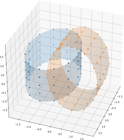
The Rings dataset consists of points lying on two interlocked cylindrical bands or “rings” orthogonal to one another and passing through one another’s centers (Fig. 2). We took a regular lattice of 60 points in and mapped it onto one of the rings in by
To generate the second ring, we rotated a copy of the first by in the -plane and translated it by along the -axis. We assigned a label of to the 60 points on the first ring and a label of to the 60 points on the second. The Rings dataset is therefore a non-linearly separable binary classification problem where the dimension of the data manifold is less than that of the linear span of the data points.
We also considered the Iris and Boston House-Prices datasets. Like Rings, Iris is a classification problem, but we one-hot encoded its labels to include a multivariate dataset with strongly correlated labels. For simplicity, following Lee et al. 2017, we implemented all three problems as regression tasks. We standardized both the input and target sets of all three datasets to help place the three problems on similar scales, as well as to set a reasonable scale for the variance hyperparameters and .
We used a single-bottleneck NNGP with one infinitely wide hidden layer before the bottleneck, bottleneck width , and post-bottleneck depth (i.e., infinitely wide hidden layers after the bottleneck) for various values of and . We equipped all hidden neurons with the normalized ReLU activation
| (8) |
The propagation of the NNGP kernel through the hidden layers given in Eq. (7) admits a closed form for the normalized ReLU activation and is given by (Cho and Saul 2009):
| (9) | ||||
where the function is defined as
Our goal is to find the bottleneck NNGP architecture (i.e., combination of bottleneck width and post-bottleneck depth ) with the greatest likelihood given a dataset of observations. We calculated the MLL of each bottleneck NNGP architecture using
| (10) |
where on the right-hand side, is the PDF in Eq. (41) of the data outputs given the data inputs and network architecture, and where the variance hyperparameters are set to their maximum likelihood estimates. We found the optimal variance hyperparameters iteratively through gradient descent. During the forward pass through the network in each iteration, we estimated the integral in Eq. (41) by drawing IID Monte Carlo (MC) samples—each an matrix with IID columns—from the pre-bottleneck NNGP. We did so using the local reparameterization trick (Kingma et al. 2015), so that each sample is actually a transformation of a draw from the -dimensional standard normal distribution. We used the Adam optimizer (Kingma and Ba 2014) to take advantage of the gradient noise generated by MC sampling during optimization; we set the initial learning rate to . In order to ensure that the noise observed in the learning curves was due only to MC sampling and not a large learning rate, we decayed the learning rate as follows: After the backward pass of each iteration, we re-evaluated the MLL using the same draw from the -dimensional standard normal distribution for the MC samples; if the new MLL was less than the value obtained from the initial forward pass of the iteration, then we multiplied the learning rate by . We iterated the optimization procedure until convergence of the MLL learning curves; once complete, we evaluated Eq. (10) once more—this time with MC samples—to obtain the final MLL estimate for each network architecture.
On all three datasets, the maximum MLL is attained at a finite bottleneck width and post-bottleneck depth ( and for Rings; and for Iris; and for Boston), thus demonstrating the utility of bottleneck layers in NNGP models (Fig. 3). On Rings and Boston, we also observe that the optimal post-bottleneck depth conditional on a bottleneck width roughly decreases as the bottleneck width increases. since the no-bottleneck NNGP kernel with ReLU activation is known to degenerate to a constant kernel with no discriminative power (Lee et al. 2017), it makes sense that a deeper network may require a narrower bottleneck to help information propagate through the network. although not conclusive from the figures alone, we believe this observation at least warrants further investigation. In Sec. 4, we do just that and find that when the variance hyperparameters are fixed, then the bottleneck width and post-bottleneck depth are indeed intimately related.


4 Bottleneck layers induce dependence
In Sec. 3.3, we showed empirically that the model likelihood of an NNGP is improved if one of the hidden layers is restricted to a finite-width bottleneck and speculated that the optimal post-bottleneck depth may increase as the bottleneck is narrowed. In this section, we investigate possible mechanisms underlying these observed trends in model performance. We start by showing that although linear correlations between distinct response variables or “output neurons” of an NNGP remain zero even in the presence of bottlenecks, the corresponding quadratic correlations are often non-zero. We also analyze the behavior of this quadratic correlation in the deep post-bottleneck limit—i.e., as the post-bottleneck depth is sent to infinity. This deep limit is distinct from the ones typically considered for DGPs, where the number of GP components is sent to infinity, and for NNGPs, where the depth of a single GP component is sent to infinity. Proposition 14 provides a striking result, which implies that bottleneck layers help a network retain discriminative power even at extreme post-bottleneck depths.
Note that in this section, we primarily consider the ReLU activation defined in Eq. (8) as it is by far the most common nonlinearity used in deep learning today. In Sec. 4.5, we briefly consider other nonlinearities and contrast their deep limit behaviors with that of the ReLU activation, thereby highlighting the peculiarities of the ReLU activation.
4.1 An exact formula for quadratic correlation
The outputs of a multi-output GP prior are IID, and it follows that the outputs of the corresponding posterior remain independent (though not necessarily identically distributed). This is a limitation of GPs for multi-task learning applications, since information cannot be shared across tasks. One method to solve this problem was proposed by Bonilla et al. 2008 who introduce a coupling matrix hyperparameter through which distinct output neurons or tasks can interact. This method, if applied to finite-width neural networks, would be superfluous since tasks could share information through a common set of features learned in the earlier layers of the network.
The key to correlating tasks in neural networks is clearly not depth alone, since the outputs of a (no-bottleneck) NNGP—however deep—are independent. Rather, following from the DGP framework as discussed in Sec. 2.1, the outputs of an NNGP become correlated if bottleneck layers are introduced, so that bottleneck NNGPs support multi-task learning out of the box. Correlation arising from finite-width bottleneck layers is exactly the type of behavior we expect in neural network architectures such as word embedding layers and many kinds of autoencoders, where the bottleneck width forces dense feature representations (i.e., feature representations that capture correlation) to be learned. The correlation structure that is induced in an NNGP prior through bottleneck layers is, however, subtle; distinct outputs of a bottleneck NNGP prior remain linearly uncorrelated (i.e., have zero covariance) but can be quadratically correlated (i.e., the squares of the outputs have non-zero covariance).
The expression for the quadratic correlation of outputs in a single-bottleneck NNGP prior can be obtained in closed form. Consider a bottleneck NNGP with one bottleneck layer of width , any number of infinitely wide hidden layers before the bottleneck, and infinitely wide hidden layers after the bottleneck. Suppose all hidden neurons (including in the bottleneck) are equipped with the normalized ReLU activation defined in Eq. (8). We also scale the bottleneck activations by in accordance with Remark 5. Let and be the bias variance and weight variance hyperparameters of both the pre-bottleneck and post-bottleneck components of the bottleneck NNGP defined as in Eqs. (4)-(5). Suppose the bottleneck NNGP is fed two inputs . Then the preactivations into the neurons in the bottleneck layer are IID with common 2D normal distribution for some covariance matrix
As is commonly done with DGPs (Damianou and Lawrence 2013; Salimbeni and Deisenroth 2017), we assume that IID Gaussian noise (with arbitrarily small) is added to the preactivations of the bottleneck layer; We include the variance of the noise in the covariance matrix , so that is invertible. We also add IID Gaussian noise to each of the two outputs of the bottleneck NNGP.
It is easy to verify that the two outputs and (for any ) are linearly uncorrelated; this immediately follows from the conditional independence of outputs given the bottleneck activations. The relationship between the squares of the outputs is, however, less trivial. Let denote the matrix of correlations between the squares of the two outputs of (the superscript is used to emphasize that the correlation is between distinct output neurons).
Proposition 10 (Quadratic correlation between outputs).
Consider the single-bottleneck NNGP with normalized ReLU activation defined above. Then
| (11) |
where and the function is defined as (Cho and Saul 2009):
The corresponding correlation is
| (12) |
where
| (13) |
Remark 11 (Quadratic correlation for stationary kernels).
In Prop. 10, if we instead consider a single-bottleneck DGP where the post-bottleneck GP has a stationary kernel (such as the RBF kernel), then the quadratic correlation between outputs is . The non-stationarity of the NNGP kernel is therefore key to capturing some amount of correlation.
The proof of Prop. 10 as well as the proofs of all other propositions in Sec. 4 are given in Appendix D. The significance of Prop. 10 is two-fold. First, quadratic correlation under the prior—although subtle—may translate to stronger dependence (such as linear correlation) under the posterior. Indeed, as stated in Remark 11, a DGP with RBF kernel captures less correlation under its prior than does a bottleneck NNGP with ReLU activation, and yet the former has been shown to be useful in modeling dependence in practice (Alaa and van der Schaar 2017; Wang et al. 2016). This suggests that a bottleneck NNGP with ReLU activation may be just as useful in modeling dependence. Second, the ability of the network to capture quadratic correlation is closely linked to its ability to operate effectively at extreme depths; we discuss this in more detail in Sec. 4.4;
The pre-bottleneck component of the bottleneck NNGP is a map that sends input vectors in to normally distributed real-valued random variables (preactivations of bottleneck neurons). By understanding covariance as an inner product on the space of finite-variance random variables, we can see that the covariance matrix is the Gram matrix of bottleneck preactivations, and the angle appearing in Prop. 10 is the angle between the preactivations of two inputs at one bottleneck neuron; we will call the bottleneck angle.
The quadratic correlation (Eq. (12)) varies with the bottleneck width roughly as and thus vanishes in the limit of infinite bottleneck width, recovering the independence of outputs of an NNGP with no bottlenecks. We empirically verified Eq. (12) for a bottleneck NNGP prior with one hidden layer before the bottleneck, one hidden layer after the bottleneck (), and with variance parameters and . We fed the example bottleneck NNGP two inputs and . Then for each bottleneck width , we generated IID samples of and used them to estimate . We repeated this simulation times, and we report the mean estimate of along with its standard deviation for each bottleneck width (Fig. 4). The empirical quadratic correlation estimates are very close to the theoretical values predicted by Eq. (12), with standard deviations all on the order of .
We performed additional simulations to understand how multiple bottleneck layers affect the correlation of outputs, as we found this to be intractable theoretically. We still consider a bottleneck NNGP with and that is fed two 2D inputs and , but now we suppose the bottleneck NNGP has 11 hidden layers (including all bottleneck layers). We chose 11 hidden layers since it allows us to restrict zero to three hidden layers to bottlenecks such that the bottlenecks are equally spaced in depth. For each of the zero to three bottleneck layers, we ran the experiment described above for a single bottleneck and estimated the quadratic correlation along with its standard deviation over ten runs for various bottleneck widths (all bottleneck layers have the same width). The quadratic correlation tends to zero with increasing bottleneck width regardless of the number of bottleneck layers, as we expect (Fig. 5). We additionally observe that for bottleneck widths , the quadratic correlation increases with the number of bottlenecks even if the overall depth of the bottleneck NNGP remains the same, suggesting that bottlenecking more layers has a similar effect to further narrowing existing bottlenecks.
4.2 Quadratic correlation as a function of depth
The inverse dependence of the quadratic correlation on bottleneck width is intuitive since we know that the outputs of an NNGP are independent in the absence of bottlenecks. There is also an interesting and less obvious dependence of the quadratic correlation on the post-bottleneck depth (where there are post-bottleneck hidden layers of infinite width) as well as on the angle between the random bottleneck preactivations of the inputs () in the bottleneck layer, as captured by the covariance matrix . We denote the quadratic correlation by to make explicit its dependence on the post-bottleneck depth and will sometimes write to further clarify its dependence on the bottleneck angle . By Prop. 10, it is easy to verify that is strictly decreasing in on with giving positive correlation, giving zero correlation, and giving negative correlation at all depths . The quadratic correlation between outputs therefore encodes the correlation of inputs in the bottleneck layer. By Eq. (13), is strictly increasing in regardless of the values of . It follows that the absolute quadratic correlation strictly decreases with for (and remains otherwise). A final property of the quadratic correlation is its range of possible values, which easily follows from the ranges of and :
| (14) |
These properties are apparent in the plot of over for an example single-bottleneck NNGP (, , ) with no pre-bottleneck hidden layers that is fed two inputs and for various values of the input angle (Fig. 6); Since there are no pre-bottleneck hidden layers, the input angle and bottleneck angle are related through the equation
Orthogonal bottleneck preactivations () and thus quadratic correlation in the example bottleneck NNGP are then achieved at an input angle . Observe in general that if , then and the range of is strictly smaller than , indicating that bias units promote positive quadratic correlation.
The behavior of (Eq. (13)) in the limit of infinite post-bottleneck depth () is easily analyzed. We have
| (15) |
This lets us determine what happens to the quadratic correlation of outputs as the number of post-bottleneck hidden layers grows to infinity.
Proposition 12 (Infinite-depth quadratic correlation between outputs).
Consider the single-bottleneck NNGP with normalized ReLU activation from Prop. 10, and suppose we send the post-bottleneck depth to infinity.
- (a)
The infinite-depth quadratic correlation matrix has -th element given by
(16) - (b)
Let be the Gram matrix of inputs with entries . If , then the mapping is invertible.
We visualize the infinite-depth quadratic correlation by plotting Eq. (16) as a function of for a single-bottleneck NNGP (, ) with no pre-bottleneck hidden layers that is fed two inputs and for various values of the input angle (Fig. 7). Note that the covariance matrix and hence the bottleneck angle are themselves functions of , which is why we plot the quadratic correlation for fixed values of instead of . The infinite-depth quadratic correlation exhibits interesting behavior around ; it is continuous but not differentiable at . The bottleneck NNGP therefore undergoes a phase transition at . The quadratic correlation tends to in the regime—meaning that the outputs of a bottleneck NNGP decouple (up through second order correlations) at infinite depth—while quadratic correlation is maintained through infinitely many, infinitely wide hidden layers in the regime , though even then the limiting correlation is weak (Eq. (14)).
A phase transition at has already been noted in the literature in the behavior of no-bottleneck NNGP models at infinite depth (Schoenholz et al. 2016; Poole et al. 2016; Lee et al. 2017). Specifically, the kernel of an NNGP with normalized ReLU activation degenerates to a constant kernel at infinite depth with a value of either if and otherwise. Bottleneck layers help to reveal a richer structure of this phase transition, as we explain next. Drawing an analogy to the classical Ising model in statistical mechanics (Baxter 2016), the hyperparameter operates as an inverse temperature with a critical value at . The quadratic correlation is then an order parameter analogous to magnetization whose derivative contains a discontinuity at the phase boundary . In the phase, the infinite-depth quadratic correlation is regardless of the bottleneck angle ; information about the inputs into the bottleneck NNGP is therefore lost, analogous to a disordered system at large scale. However, as crosses the phase boundary from below, the system undergoes a symmetry breaking with the infinite-depth quadratic correlation taking a distinct value for each bottleneck angle as well as for each input angle . This lets us recover information about the inputs from the infinite-depth quadratic correlation, indicating that bottlenecks help information propagate to extreme depths (Prop. 12 (b)).
The symmetry breaking discussed above is not apparent in the phase transition of degenerate NNGP kernels noted in the literature; i.e., all information about the inputs are lost in an infinite-depth (no-bottleneck) NNGP in either phase. We see, however, that the restriction of just one hidden layer to a bottleneck is sufficient to break this symmetry. Moreover, the symmetry can be recovered by sending the bottleneck width to infinity (Thm. 8); the bottleneck is therefore analogous to an external magnetic field in the Ising model.
4.3 A divergent depth scale
Schoenholz et al. 2016 show that the characteristic depth scale on which the kernel of a (no-bottleneck) NNGP degenerates exponentially to its deep limit diverges at a phase boundary in -space, and they use this result to argue that values of near criticality or “at the edge of chaos” optimize trainability by maximizing the depth to which information can penetrate in an NNGP. We show that the depth scale on which the quadratic correlation converges to its limit also diverges at the phase boundary .
Proposition 13 (Characteristic depth scale).
Consider the single-bottleneck NNGP with normalized ReLU activation from Prop. 10, and suppose it is fed two inputs and with and bottleneck angle . Then for all positive , the quadratic correlation is asymptotically exponential in , meaning that the limit
| (17) |
exists and is finite and non-zero for some , which we find to be
| (18) |
In the case , the limit is infinite for all finite .
Proposition 13 excludes the case of orthogonal bottleneck preactivations () since it leads to trivial asymptotic behavior ( for all ). The quantity given in Eq. (18) is called the characteristic depth scale and is proportional to the “half-life” of quadratic correlation at large depth. The divergence of the depth scale at gives us another perspective on the phase transition in bottleneck NNGP models (Fig. 8). Based on this, we expect optimal values of the hyperparameter to be greater than but close to ; although gives the smallest decay rate (i.e., largest depth scale) to the infinite-depth quadratic correlation, this limiting value is . Larger values of admit non-zero infinite-depth quadratic correlations, but values that are too large lead to fast decay rates (i.e., small depth scales). We hypothesize that this tension between large depth scales (near ) and non-zero quadratic correlations () is the main driving force determining the optimal value of in the phase.
4.4 Non-degenerate kernels at extreme depths
The non-trivial dependence of the infinite-depth quadratic correlation on the bottleneck angle has remarkable implications for the kernel or covariance matrix of individual output neurons of a bottleneck NNGP at infinite depth. Consider again the single-bottleneck NNGP described at the beginning of Sec. 4.1, and suppose it is fed two linearly independent inputs and . Assume that the infinite-depth kernel is degenerate so that the associated correlation matrix is a matrix of ones; this is indeed the case when there are no bottlenecks, where the correlations in tend to 100% even when all elements of the kernel grow to infinity at infinite depth. Then the outputs and of a single output neuron at infinite depth are linearly dependent and are in fact equal. It follows that the elements of the quadratic correlation matrix between distinct output neurons are all equal, but this is impossible in the phase since is a one-one function of (Fig. 7) and the diagonal elements assume while the off-diagonal elements assume (since and are linearly independent). We therefore learn that the kernel of an NNGP does not degenerate to a constant in the phase if at least one hidden layer is bottlenecked.
Unfortunately, the kernel—and thus the associated correlation matrix—of each output neuron of a bottleneck NNGP do not admit closed forms, even in the infinite depth limit. The quadratic correlation matrix (without a superscript ) for individual outputs is intractable as well, but its infinite depth limit does admit an elegant closed form.
Proposition 14 (Infinite-depth quadratic correlation for single output).
Consider the single-bottleneck NNGP with normalized ReLU activation from Prop. 10, and suppose we send the post-bottleneck depth to infinity.
- (a)
The infinite-depth quadratic correlation matrix of a single output neuron has -th element given by
(19) - (b)
Let be the Gram matrix of inputs with entries . If , then the mapping is invertible.
The infinite-depth single-output quadratic correlation carries many of the same properties as the infinite-depth between-output quadratic correlation . Recalling that as , it is easy to verify that . The single-output quadratic correlation also exhibits the same symmetry breaking at the phase boundary as the between-output quadratic correlation; this is evident in the example plot of as a function of , using the same setup as for Fig. 7 (see Fig. 9).
In the phase , the single-output quadratic correlation is 100%, suggesting degeneracy at infinite depth. In contrast, in the phase —where symmetry breaks— becomes a strictly increasing function of the input angle , allowing us to recover some information about the inputs (Prop. 14 (b)). In particular, Prop. 14 (b) implies that in the ordered phase , if the norms of the inputs are known (if the inputs are constrained to a sphere, for example), then the input angle can be recovered from the single-output quadratic correlation even at infinite depth. This stands in stark contrast to no-bottleneck NNGP models, where all information is lost at infinite depth regardless of the phase, and it suggests that bottleneck layers are vital for the trainability of very deep models.
4.5 Other nonlinearities
The behavior described in Prop. 14 does not extend to other common nonlinearities and is thus all the more striking. Two notable examples are the sigmoidal nonlinearity and the sinusoidal nonlinearity
| (20) |
The significance of the latter is that the corresponding NNGP has an RBF kernel; the random features literature (Rahimi and Recht 2008; Cutajar et al. 2017) hints at this connection but does not discuss it in the context of NNGPs or neural network nonlinearities. We make this connection more precise in the next proposition and subsequent remark (see Appendix D.1 for the proofs of both Props. 15, 17).
Proposition 15 (RBF-NNGP kernel recursion).
Consider an NNGP mapping to with hidden layers and the sinusoidal nonlinearity in Eq. (20).
- (a)
The NNGP kernel for the -th hidden layer is given recursively as
(21) (22) for where is the kernel of the output layer.
- (b)
In the deep limit , the NNGP kernel converges pointwise to
(23) where
(24) (25)
Remark 16 (RBF-DGP as a bottleneck NNGP).
Since the sinusoidal nonlinearity in Eq. (20) clearly satisfies the linear envelope condition, then we can apply Thm. 4 to a BNN with the sinusoidal nonlinearity and obtain a bottleneck NNGP limit. If no bottlenecks are imposed, then the wide limit of such a BNN is the NNGP described in Prop. 15. In particular, using Eqs. (21)-(22), the single-hidden-layer NNGP with sinusoidal nonlinearity has kernel
which we recognize as the RBF kernel. More generally, if the BNN with sinusoidal nonlinearity has an odd number of hidden layers and the -th hidden layers are restricted to bottlenecks for , then the bottleneck NNGP limit is a DGP with GP components each with RBF kernel (and sinusoidal nonlinearities applied to the bottleneck layers).
The deep limit of an NNGP with sinusoidal nonlinearity is described in Prop. 15 (b). It is identical to the behavior of an NNGP with sigmoidal nonlinearity as described by Poole et al. 2016, except that and take different forms and the phase boundary has a different location. In one phase ( for the sinusoidal nonlinearity), all inputs tend to correlation as depth is increased without bound—similar to the ReLU activation. However, in the other phase ( for the sinusoidal nonlinearity)—the “chaotic phase”—the infinite-depth correlation for distinct inputs is a constant less than ; thus, unlike the ReLU activation, the sigmoidal and sinusoidal nonlinearities allow distinct inputs to remain distinct through infinite depth, although all information about the distince between distinct inputs is lost. Moreover, the introduction of a bottleneck does not remove this degeneracy—in sharp contrast to Prop. 14. We substantiate this with the next proposition.
Proposition 17 (Deep post-bottleneck limit for sigmoidal and sinusoidal nonlinearities).
Consider a single-bottleneck NNGP mapping to with either sigmoidal or sinusoidal nonlinearity . Suppose IID Gaussian noise is added to the outputs for any . Given two distinct inputs , let be the PDF of , where is the post-bottleneck depth. Then in the deep post-bottleneck limit , the PDF converges pointwise to
| (26) |
where is a matrix with entries with given in Eq. (23).
Note that Eq. (26) is independent of bottleneck width; in fact, it is exactly the PDF of a no-bottleneck NNGP, indicating that the bottleneck has no effect at all on the deep post-bottleneck limit given either the sigmoidal or sinusoidal nonlinearity. In contrast to Prop. 14 (b) for the ReLU activation, the only information about the inputs that can be recovered from the deep post-bottleneck limit is whether the inputs are distinct. This suggests a fundamental difference between the ReLU activation and the sigmoidal nonlinearity and between the NNGP kernel with ReLU activation and the RBF kernel—namely, that the ReLU activation allows a network to operate at very large depths as long as one bottleneck is present. Classifying activation functions based on their deep limit and deep post-bottleneck limit behaviors could help to better understand which activation functions are useful in practice and is a topic for future work.
4.6 Other deep limits
Besides the deep post-bottleneck limit discussed in Secs. 4.2-4.4, there are two other limits we could have considered: 1) The deep pre-bottleneck limit where a single-bottleneck NNGP has infinitely many infinitely wide hidden layers before its bottleneck but only finitely many after, and 2) the doubly deep bottleneck limit where the single-bottleneck NNGP has infinitely many infinitely wide hidden layers both before and after its bottleneck. The quadratic correlation between the activations of distinct output neurons can be analyzed in both of these limits by replacing the pre-bottleneck NNGP covariance matrix in Prop. (10) with a sequence of such covariance matrices indexed by the pre-bottleneck depth. Since the NNGP kernel with ReLU activation tends to a constant in the deep limit, then the bottleneck angle tends to in both the deep pre-bottleneck limit and doubly deep bottleneck limit. Although the quadratic correlation remains nontrivial in both limits and even exhibits a first-order phase transition at in the doubly deep bottleneck limit, these results are uninteresting as all information about the original inputs into the network is lost due to vanishing bottleneck angle.
The quadratic correlation between the activations of a single output neuron at two different inputs can also be analyzed in both the deep pre-bottleneck and doubly deep bottleneck limits; calculations proceed similarly as in the proof of Prop. 14. Again, since the bottleneck angle tends to , we find that the quadratic correlation tends to 100% in both limits at every post-bottleneck depth; the bottleneck NNGP kernel therefore degenerates, unlike in the deep post-bottleneck limit. We conclude that out of the three possible deep limits, only the deep post-bottleneck limit is interesting since it is the only one that admits a phase () in which information about network inputs is preserved.
5 Conclusion
Our main theorem, Thm. 4, generalizes the result of 17 concerning deep neural networks whose hidden layer widths are increased without bound to a setting in which some intermediate hidden layers, called bottlenecks, are fixed to a finite width. From a theoretical perspective, this result connects the NNGP literature with that of DGPs, as the resulting probability model is in fact a DGP consisting of a composition of NNGP components. Additionally, we have explored the effect of these bottleneck layers on the resulting probability model from a practical perspective, showing that model likelihood peaks at a finite bottleneck width and is superior to that of no-bottleneck NNGPs.
Surprisingly, in contrast to no-bottleneck NNGP models, the behavior of a bottleneck NNGP with ReLU activation at extreme post-bottleneck depths is not always degenerate (Props. 12, 14); in particular, the input Gram matrix can be fully recovered from the between-output quadratic correlation matrix of the bottleneck NNGP at infinite post-bottleneck depth, and the input angle can be recovered even from the single-output quadratic correlation matrix at infinite depth if the input norms are known. Bottleneck layers are therefore fundamental as they allow networks to “go deeper”. However, this non-degeneracy in the deep limit manifests only when the network weight prior is weaker than a standard normal. We have just begun to explore the dependence of the deep post-bottleneck limit on the prior weight variance, showing that convergence to the limit is asymptotically exponential in depth and that the characteristic depth scale diverges at a critical value of the weight prior variance.
So far, we have not directly connected bottleneck NNGPs with BNNs, aside from studying the limits of BNNs in the wide regime. However, an interesting special case of bottleneck NNGPs emerges when every hidden layer is fixed at finite width. The result is a BNN, but our result lends an interesting perspective that suggests that one might approach BNN inference with a non-parametric DGP-based approach. Indeed, in follow-up work we intend to explore the practicality of such a method. Moreover, we believe that our main theorem can easily be extended to convolutional architectures (by introducing a second index for each hidden layer), and thus we plan to explore the implications of our work for convolutional BNNs.
Finally, in this work we did not consider the implications of the bottleneck NNGP for the learning dynamics of Gaussian-initialized deterministic neural networks (DNNs). It is now a celebrated result that the evolution over training time of a Gaussian-initialized DNN is described in the wide limit by an exactly solvable linear ODE, where the time evolution operator is termed the neural tangent kernel (NTK) and is related to the NNGP kernel (Jacot et al. 2018). As part of additional follow-up work, we plan to investigate the “bottleneck NTK”, where the wide limit is relaxed to allow for some bottleneck layers. The result is a system of coupled ODEs that is more challenging to analyze but carries potential for a more refined description of the evolution of finite-width DNNs.
acknowledgments-disclosure-of-funding.
This work has been supported in part by the Joint Design of Advanced Computing Solutions for Cancer (JDACS4C) program established by the U.S. Department of Energy (DOE) and the National Cancer Institute (NCI) of the National Institutes of Health. This work was performed under the auspices of the U.S. Department of Energy by Argonne National Laboratory under Contract DE-AC02-06-CH11357, Lawrence Livermore National Laboratory under Contract DEAC52-07NA27344, Los Alamos National Laboratory under Contract DE-AC5206NA25396, and Oak Ridge National Laboratory under Contract DE-AC05-00OR22725. Research sponsored by the Laboratory Directed Research and Development Program of Oak Ridge National Laboratory, managed by UT-Battelle, LLC, for the US Department of Energy under contract DE-AC05-00OR22725. This research used resources of the Compute and Data Environment for Science (CADES) at the Oak Ridge National Laboratory, which is supported by the Office of Science of the U.S. Department of Energy under Contract No. DE-AC05-00OR22725. The United States Government retains and the publisher, by accepting the article for publication, acknowledges that the United States Government retains a non-exclusive, paidup, irrevocable, world-wide license to publish or reproduce the published form of the manuscript, or allow others to do so, for United States Government purposes. The Department of Energy will provide public access to these results of federally sponsored research in accordance with the DOE Public Access Plan (http://energy.gov/downloads/doe-public-access-plan).Appendix A Convergence of stochastic processes
Here we define three notions of convergence that are important for formally stating and proving the bottleneck NNGP limit. The first notion of convergence is the one that 17 employ to prove the (no-bottleneck) NNGP limit. They consider a sequence of BNNs mapping to restricted to a countable set of inputs . Each BNN is then equivalent to a random sequence of -vectors, i.e. a random variable taking values in . Following Billingsley 1999, 17 equip the sequence space with the metric
where . The metric induces the Euclidean topology on , and we endow with the associated Borel algebra , giving us a measurable space of sequences. Demonstrating convergence in can prove challenging, but 17 simplify the task by invoking the following theorem.
Theorem 18 (Billingsley 1999).
A sequence of stochastic processes with countable index set converges in distribution to a stochastic process on the measurable space if and only if every sequence of finite-dimensional marginals converges in distribution to the corresponding limiting marginal .
Theorem 18 effectively reduces the task of proving the convergence of a sequence of random sequences to that of a sequence of random vectors. When looking at the convergence of -dimensional marginal distributions, it is convenient to introduce the following notation.
Definition 19 (Batch stochastic process).
Let be a stochastic process. Then the batch stochastic process of size associated with is the stochastic process defined by
By working with batch stochastic processes, we can think of inputs as constituting a single input. Thus, to show , it is enough to show for each input for every batch size .
Our proof of the bottleneck NNGP limit takes the approach of showing that each component of a BNN after the first bottleneck layer converges to an NNGP in the wide limit with some uniformity. We specify the appropriate notion of uniform convergence next.
Definition 20 (Uniform convergence in distribution (Sweeting 1980)).
A sequence of stochastic processes is said to converge in distribution to uniformly on if for every continuity set of , i.e., a set satisfying
we have the limit
We denote this by .
Note that uniform convergence in distribution is distinct from and is not a stronger version of convergence in distribution in since the former notion concerns only the singly-indexed marginals of a stochastic process while the latter deals with the joint distribution of all elements of a stochastic process. However, the uniform convergence in distribution of the batch stochastic processes is stronger than the convergence in distribution of the original stochastic processes . Proving uniform convergence in distribution can be challenging, but fortunately there is another closely related notion of convergence, which we define next.
Definition 21 (Continuous convergence in distribution (Sweeting 1980)).
Let be a topological space. A sequence of stochastic processes is said to converge in distribution to continuously on if for every and sequence converging to , the sequence of random variables converges in distribution to . We denote this by .
Uniform and continuous convergence in distribution are related through the following proposition.
Proposition 22 (Saikkonen 1993).
Let be a topological space. Let be a sequence of stochastic processes and a stochastic process. Then the following are equivalent statements:
- (a)
.
- (b)
on every compact subset of and is a continuous function for every continuity set of .
We should mention that Sweeting 1980 and Saikkonen 1993 do not state Defs. 20-21 and Prop. 22 directly but instead define and work with the equivalent notions of uniform and continuous weak convergence of probability measures. The proof of Prop. 22 is a simple application of the equivalence of uniform and continuous convergence of real-valued functions on compact sets.
Appendix B The bottleneck NNGP theorem
Here we list the proof of our main theorem (Thm. 4) along with all supporting lemmas. We give a sketch of the proof next, highlighting the role of each lemma and its position in the general proof strategy.
The first step is to apply Thm. 18 so that it is sufficient to prove convergence of BNNs to a bottleneck NNGP restricted to an arbitrary finite set of inputs. Since each component in Thm. 4 is being evaluated at inputs, then it is convenient to utilize the concept of a batch stochastic process of size (Def. 19). By working with batch BNNs, we can think of inputs as constituting a single “batch” input. This reduces our task to proving the convergence of batch BNNs to a batch bottleneck NNGP given a single arbitrary input.
The next step is to find sufficient conditions under which the distributional limit of an element-wise composition of a sequence of stochastic processes with a sequence of random variables equals the composition of the limiting stochastic process with the limiting random variable. This trick can then be iterated via induction to prove that the limit of compositions is the composition of limits for stochastic processes. Lemma 24 provides such sufficient conditions, which include a notion of uniform convergence in distribution (Def. 20).
Proving Thm. 4 now comes down to verifying the conditions of Lemma 24. Condition (a) is given to us by Thm. 3 for single-bottleneck networks and holds by induction for multi-bottleneck networks. Condition (b) is also immediate in the single-bottleneck case, although it is less obvious for multi-bottleneck architectures. We verify condition (b) directly in the proof of Thm. 4 but take aid from Lemma 25. Lemma 26 establishes condition (c), which amounts to showing that the NNGP kernel is a continuous function. Condition (d) is the trickiest to verify; it states that the outer sequence of stochastic processes (that is composed with an inner sequence of random variables) must converge in distribution uniformly (Def. 20) on compact sets, meaning that the rate of convergence in distribution should be independent of the input to the stochastic processes. Condition (d) is verified with the help of Lemma 27.
Lemma 27 is a direct generalization of Lemma 12 in 17; the latter states that given a fixed finite batch of inputs, BNNs with no bottlenecks converge in distribution to an NNGP in the wide limit. In Lemma 27, we strengthen the mode of convergence to continuous convergence in distribution (Def. 21). More specifically, Lemma 27 states that a BNN converges in distribution to an NNGP even if we replace the fixed batch of inputs with a convergent sequence of input batches. Continuous convergence in distribution is in fact equivalent to uniform convergence in distribution on compact sets (Prop. 22), thus granting condition (d).
The proof of Lemma 27 runs in parallel to the proof of Lemma 12 in 17. It depends on several lemmas (Appendices B.3-B.4) that are all simple extensions of (or help to extend) the lemmas in 17; at each step, we simply replace the fixed batch of inputs in 17 with a convergent sequence of input batches and verify that convergence in distribution still holds. Only a few key modifications are made to the lemmas establishing uniform integrability (Appendix B.4).
B.1 Notation
We start with some notation. Let be a sequence of BNNs each with hidden layers of widths , , and nonlinearity that satisfies the linear envelope condition. Let be the limiting NNGP of the sequence of BNNs. Let (resp. ) and (resp. ) be the preactivation and activation of the -th neuron in the -th hidden layer of (resp. ).
For each , let be a batch of inputs, and suppose the sequence of batches converges to some finite . Let be a countably infinite block vector whose blocks are indexed by and where each block has elements. Let have finite support , where is a finite subset of ; i.e., only finitely many blocks indexed by are permitted to have non-zero elements. Let denote the -th element in the -th block. For each , define the preactivation projections of a BNN and its limiting NNGP as
Let be the NNGP kernel of . The kernel relates to the block kernel (Eqs. (6)-(7)) through the equation
where is the identity matrix, is the countably infinite identity matrix, and denotes the Kronecker product. We also define
which satisfies the relation
We let denote a block matrix where is the -th block. The block matrices and for have infinitely many blocks since the NNGP has infinitely wide hidden layers. However, given a block vector of finite support , the quadratic forms and are still finite sums:
We define a quadratic form for similarly.
Next we define the quantities that are at the heart of the proof of Lemma 27. This definition is similar to Definition 7 in 17. We discuss the purpose of this definition in more detail in Appendix B.3 in the context of the Central Limit Theorem.
Definition 23 (Projections and summands).
For each and for each and , define the summands
| (27) |
and the projections
| (28) |
Finally, for , define the variances
| (29) | ||||
| (30) | ||||
B.2 Main lemmas and theorem
This section contains the proof of the main theorem (Thm. 4) as well as all original lemmas supporting it. See the proof sketch in Sec. 3.1 for an overview and guide to the logical flow of the lemmas. We start with a lemma that gives sufficient conditions under which the distributional limit of a sequence of compositions of stochastic processes and random variable indices equals the composition of limits.
Lemma 24 (Limit of stochastic process compositions).
Let be a sequence of random vectors and a random vector of dimension . Let be a sequence of stochastic processes and a stochastic process with . If
- (a)
converges in distribution to , denoted ,
- (b)
is eventually bounded,
- (c)
is a continuous function, and
- (d)
on every compact ball in centered at ,
then the sequence of random variables .
Proof.
We first prove the claim for the case that and are real-valued stochastic processes () and for all . For this case, we will use the notation in place of to emphasize that is a scalar.
Let be a continuity point of . We want to show that
Let . We have
| (31) |
We will show that both terms on the right-hand side of Inequality (31) tend to .
We start with the second term. Let and be the probability distributions associated with and , respectively. Then the second term becomes
Since with , then we have
where is the cumulative distribution function (CDF) of the standard normal distribution. Since is continuous, then the map is immediately seen to be continuous as well. Moreover, is clearly bounded. Since , then converges weakly to , so that
Therefore, there exists an integer such that
| (32) |
We next bound the first term on the right-hand side of Inequality (31). We have
| (33) |
We will bound the integrand. Since is eventually bounded, then there exists and an integer such that
Define
is defined such that implies
We therefore have
| (34) |
Since follows a normal distribution, then is trivially a continuity point of for every . Since converges in distribution to uniformly on every zero-centered compact ball, then there exists an integer such that
Since , then we have the weaker bound
Combining this with Eq. (34) gives
Using this bound in Inequality (33), we get
| (35) |
Now consider the more general case where the processes and take values in for and where the kernel of is not necessarily strictly positive definite. Consider any , and define the processes
where is independent of and . and are real-valued stochastic processes and is normally distributed with variance
By the case already proven above, . Since the addition of an independent normally distributed random variable preserves convergence in distribution, then . Since this holds for any vector , then by the Cramér-Wold Device (Billingsley 1995), we obtain the conclusion . ∎
Lemma 24 can be applied inductively to show that a sequence of compositions of stochastic processes converges in distribution to the composition of limit processes. The next lemma verifies condition (b) of Lemma 24.
Lemma 25 (Uniformly bounded neural network variances).
Let be a sequence of BNNs mapping to with hidden layers of widths , , and nonlinearity on the -th hidden layer satisfying the linear envelope condition. Then for every , the sequence of second moments is uniformly bounded by for some constants .
Proof.
Let . The claimed uniform bound on holds if we can uniformly bound for each . Since , then we need to establish for sufficiently large . We proceed by induction on . In the case , we have
Taking and , this is clearly bounded by independently of . By exchangeability, this same bound holds for all .
Now suppose for some that the claimed uniform bound holds. We then need to establish the bound for some . We have
where is the probability distribution of . By the linear envelope condition,
which is clearly bounded by an expression of the form independently of for some . The claim then follows by induction. ∎
The next lemma verifies condition (c) of Lemma 24, which amounts to showing that the NNGP kernel is continuous.
Lemma 26 (Continuity of batch NNGP kernel).
Let be an NNGP with hidden layers and nonlinearity that satisfies the linear envelope condition. Then the associated batch NNGP of size has marginal , where the batch NNGP kernel given by is a continuous function.
Proof.
All we need to show is that is a continuous function. Since , then it is sufficient to show that the NNGP kernel is continuous. We do so inductively by showing that is continuous for , where .
For , is clearly continuous. Now suppose for some , that is continuous. We then need to show that is continuous. Let be a convergent sequence of pairs of inputs such that . Since is continuous, then . Let (resp. ) denote the -th column of the symmetric positive semidefinite square root (resp. ) of (resp. ). Then by the work of Cho and Saul 2009, the kernel recursion in Eq. (7) can be expressed as
and is given similarly. To ensure continuity, we will show that . We do so by verifying the conditions of the Dominated Convergence Theorem. First, by the linear envelope condition, there exist positive constants and such that
where denotes the Frobenius norm. Since the matrix square root operation is continuous under the Frobenius norm, then is bounded by some . We therefore have
hence
where the bound on the right-hand side is clearly integrable over . Moreover, since the matrix square root operation is continuous and is continuous, then
| (36) |
Therefore, by the Dominated Convergence Theorem, so that is continuous. The continuity of the kernel then follows by induction. ∎
The next lemma will help to verify condition (d) of Lemma 24. It is a generalization of Lemma 12 in 17 and depends on several additional lemmas (Appendices B.3-B.4) similar to those in 17.
Lemma 27 (Continuous convergence in distribution of batch BNNs).
Consider a sequence of BNNs mapping to with hidden layers of widths , , and nonlinearity that satisfies the linear envelope condition. Let be the NNGP limit of the BNNs as given by Thm. 3. Then for any , the corresponding sequence of batch BNNs converges in distribution to the batch NNGP continuously.
Proof.
For each , let be a batch of inputs such that the sequence of batches converges to some finite . We need to show that converges in distribution to continuously, i.e. that the sequence of random variables converges in distribution to and thus
| (37) |
We will do so by establishing inductively for every .
For the case , let with finite support .
By definition (Eq. (1)), it is straightforward to verify that
Let be a continuity point of so that if . Extend the CDF of the standard normal distribution by setting and . Then the map
| (38) |
is continuous on and is right-continuous at if . Now since the kernel is a continuous function (Lemma 26) and since , then . Moreover, since we just established that the map given by Eq. (38) is continuous, then it follows that
and hence . By the Cramér-Wold Device, we deduce that .
Now suppose that for every finite subset and for some . We then want to show that this same convergence holds for . Let with finite support . We view as a block vector where is the -th element in the -th block. By Lemmas 31-33, the sequence of summands for satisfies the conditions of Thm. 30; condition 1 is immediate since the weights and are independent and have mean . Theorem 30 then tells us that the projections , where the limiting variance is given by (Eq. (30)). By the Cramér-Wold Device, this implies
which in turn implies
Equation (37) then follows by induction, thus establishing continuous distributional convergence. ∎
Next is the proof of the bottleneck NNGP theorem, which is the main theorem of our paper.
Proof of Thm. 4.
We proceed by induction on . The case is given to us by Thm. 3 (i.e., no hidden bottlenecks). Now suppose the claim holds for some . We will prove the claim for the case .
Let be a finite subset of . Define the random variables
Let (resp. ) be the batch BNN (resp. batch NNGP) corresponding to (resp. ), and observe that
We proceed to establish the four conditions of Lemma 24 in order to prove
| (39) |
By the inductive hypothesis, in and thus in particular , establishing condition (a). Observe that
Since a composition of BNNs is still a BNN (with some hidden layers having linear activation), then we can apply Lemma 25 to each expectation in the sum to get the bound
for some constants . In other words, the sequence of second moments of is bounded, establishing condition (b). Lemma 26 gives us condition (c). Finally, Lemma 27 tells us that . By Prop. 22, we immediately have on every compact subset of , establishing condition (d).
Remark 28 (Nonlinear bottleneck).
Theorem 4 holds even if we replace and with and respectively for . The proof is nearly identical, making the necessary replacements where appropriate. The only additional step needed is to verify condition (c) of Lemma 24 for in the inductive step; by Lemma 24, and hence by Prop. 22. Now since is (sequentially) continuous, then whenever . By Prop. 22, , establishing condition (c).
Remark 29 (Discontinuous nonlinearity).
Theorem 4 holds even if the nonlinearity is continuous only almost everywhere (AE), as long as is continuous at or . If is continuous AE, then the pointwise convergence in Eq. (36) holds AE, which is still sufficient for the Dominated Convergence Theorem. Moreover, the Continuous Mapping Theorem used in Lemmas 31-33 is still applicable as long as the set of discontinuities of has measure with respect to the distribution of the NNGP preactivation . If , then it becomes possible for the distribution of to degenerate to a delta distribution concentrated at ; if is also discontinuous at , then its set of discontinuities will have measure with respect to the delta distribution, hence the requirement that if is discontinuous at .
B.3 Verifying the conditions of the CLT for exchangeable processes
The results in this section serve to support the proof of Lemma 27. Since Lemma 27 is similar to Lemma 12 in 17, then the results in this section are also similar to results in 17. The approach to proving Lemma 27 is to show that in the (no-bottleneck) NNGP limit, if the preactivations into one hidden layer converge in distribution continuously to a GP, then so do the preactivations into the next hidden layer. This is done using a special central limit theorem. The challenge is that the preactivations into any hidden layer after the first hidden layer are independent only in the wide limit. Moreover, the distribution of each preactivation changes as the preceding hidden layer grows in width. The following is a central limit theorem adapted specifically for this case; it is a restatement of Lemma 10 in 17, which is in turn an adaptation of a central limit theorem for exchangeable processes by Blum et al. 1958.
Theorem 30 (CLT for sequences of exchangeable sequences (17)).
For each positive integer , let be an exchangeable sequence of random variables with mean , variance , and finite absolute third moment. Suppose also that the variances converge to the limit If
- (a)
,
- (b)
, and
- (c)
then for any strictly increasing sequence , the sequence of standardized partial sums with
converges in distribution to , where is interpreted as the constant .
We will apply Thm. 30 to the summands (Eq. (27)) to show that the projection (Eq. (28)) converges to a GP. This requires us to verify the conditions of Thm. 30. We verify the existence of the limit first. The following lemma is analogous to Lemma 11 in 17. The main difference is that the batch input is replaced with a convergent sequence of input batches . We maintain the notation introduced in Sec. B.1.
Lemma 31.
Proof.
It is clear that since the weights have mean. We therefore have
Theorem 3.5 in Billingsley 1999 tells us that a limit can be moved inside an expectation operator if the sequence inside the expectation converges in distribution and is uniformly integrable. Since the preactivations converge in distribution and since the nonlinearity and multiplication mapping to are continuous functions, then the Continuous Mapping Theorem implies that the products of activations in the above expectations also converge in distribution. Uniform integrability holds by Cor. 39. We therefore have the limit
completing the proof. ∎
Condition (a) of Thm. 30 is easily verified directly in the proof of Lemma 27. We thus move to condition (b). The following lemma is analogous to Lemma 15 in 17.
Lemma 32.
Suppose that for some . and for every finite set . Then
Proof.
We proceed in direct analogy to the proof of Lemma 31. We have
Since the preactivations converge in distribution for , and since the nonlinearity and multiplication from to are continuous functions, then the Continuous Mapping Theorem implies the four-way products of activations in each expectation above converge in distribution as well. Corollary 38 also tells us that the set of these four-way products of activations is uniformly integrable. By Theorem 3.5 in Billingsley 1999, we have the limit
| (40) |
Since parallel activations in a layer decorrelate in an NNGP, then we have
completing the proof. ∎
Lemma 33.
Suppose that for some , and for every finite set . Then
Proof.
We will prove the stronger result that the third absolute moment of is bounded over . By Hölder’s inequality,
Thus, to bound the left side independently of , it is sufficient to do the same for the fourth moment of . Observe that
where the right-hand side is similar to the quantity discussed in Lemma 32. Therefore, calculations proceed in direct analogy to the proof of Lemma 32 up to and including Eq. (40). Thus, we have
The right-hand side can be shown to be finite by applying Lemma 35 to bound the expectation of the four-way product by a product of eighth moments, applying the linear envelope property to obtain bounds in terms of preactivations, and finally noting that the eighth moment of a normal distribution is finite; this gives us the desired bound on the fourth and hence third absolute moment. ∎
B.4 Establishing uniform integrability
The results in this section serve to support the proofs in Appendix B.3. As in Appendix B.3, the results in this appendix are stronger versions of results appearing in 17. The key results in this section are Lemma 35 and Cors. 38 and 39 and are the only ones referenced outside of this section.
Lemma 34.
Let be a random variable. Then .
Proof.
By Hölder’s Inequality, we have
∎
The following lemma is a stronger version of Lemma 18 in 17. 17 proves that the expectation is uniformly bounded by a polynomial in the eighth moments for without specifying the polynomial. Lemma 35 below provides the explicit bound , which is a polynomial in the eighth moments. This bound is important when proving uniform convergence with respect to the inputs of a random neural network, since the coefficients and exponents in the bound are independent of the network’s input.
Lemma 35.
Let be random variables with for . Then for any choice of it holds that
Proof.
Using Hölder’s inequality twice, we have
If , then , which can be written as . If , then by Lemma 34, . If , then we simply have . We therefore see that for any , . Substituting this into the above product yields the desired bound. ∎
The following lemma extends Lemma 20 in 17 to stochastic processes in the sense that the input into the BNN is now a variable. We can achieve a uniform bound if we assume that the input space is compact.
Lemma 36.
Let be a compact input space. Then for each , the eighth moments of the normally distributed random variables defined by equation (1) are uniformly bounded over all , and .
Proof.
We proceed by induction on . The case is trivial; the random variables are IID over and follow the normal distribution . The eighth moments are therefore
Clearly the eighth moment is independent of and . Moreover, since is compact, then . The eighth moments are therefore uniformly bounded over , and .
Now assume that the eighth moments of are uniformly bounded over , and for all and for some . We wish to prove that the eighth moments of are uniformly bounded over , and . Using the inequality for elements and of the space for , which follows from the convexity of for , the bound
is first established. The term is bounded since the biases are normally distributed. Moreover, the biases are IID over and are independent of . Therefore, to achieve the desired uniform bound, we only need to show that the term
is uniformly bounded over , and . By Lemma 20 in 17,
where are constants from the linear envelope property of the activation function. Letting and multiplying out the quantity in the above expectation, we have
Using Lemma 35 and the fact that the moments of are independent of by exchangeability, we have
where each is a rational number between and . Define the function
and note that and the are independent of the hidden width index , the hidden neuron index , and the input . Moreover, is increasing on the interval . Since we assumed as our inductive hypothesis that , then it follows that
implying that uniformly over , and , thereby completing the proof. ∎
The following lemma extends Lemma 21 in 17 to stochastic processes in the same sense as Lemma 36 above.
Lemma 37.
Let be a compact input space. Then for any and indices , the set of random variables
is uniformly integrable.
Proof.
By the de la Vallée-Poussin Theorem (Meyer 1966, p.19, Theorem T22), is uniformly integrable if
We consider . By Lemma 35,
where we obtained the last line by exchangeability over the indices . We therefore have
It thus suffices to show that the supremum in the last line is finite. By the linear envelope property of the activation function,
By Lemma 36, the right-hand side is uniformly bounded over all and , completing the proof. ∎
Corollary 38.
Let for be four convergent sequences with finite limits. Then for any and indices , the set of random variables
is uniformly integrable.
Proof.
Since the sequences for , converge to finite limits, then there exists a compact set that contains for all and . By (the proof of) Lemma 37, we have
where the are elements of the compact set . It then holds in particular that
Uniform integrability then follows by the de la Vallee-Poussin Theorem. ∎
Corollary 39.
Let for , be two convergent sequences with finite limits. Then for any and indices , the set of random variables
is uniformly integrable.
Proof.
By the de la Vallée-Poussin Theorem, is uniformly integrable if
We consider . We have
which is finite by (the proof of) Cor. 38. The claim then follows. ∎
Appendix C Correspondence to the no-bottleneck NNGP
The following is our proof of the Wide Bottleneck Correspondence Theorem for the case of a single-bottleneck NNGP.
Proof of Thm. 8.
First we prove statement (b). We will do so for ; the case proceeds similarly. Let be a finite set of inputs. Let and be the PDFs of and , respectively. Let and be the NNGP kernels of the pre-bottleneck and post-bottleneck components (with respective depths and ) of ; note that the kernels are independent of . Then the PDF is given by
| (41) |
where is the vector of preactivations into the -th hidden neuron in the bottleneck, and where we use the notation to mean the normal PDF in the variable with mean and covariance . Observing that the NNGP kernel in Eqs. (6)-(7) depends on its inputs only through their Gram matrix and writing the kernel of the first layer explicitly, we can define a function on the space of symmetric positive semidefinite matrices such that
Defining the random matrix
| (42) |
and letting denote the probability measure associated with , the PDF in Eq. (41) can be written as
Here is a dummy variable. Now since the in Eq. (42) are IID, then so are the matrices . Therefore, is an empirical average of IID random matrices. By the Law of Large Numbers, we have
where the convergence is in probability. In particular, so that the sequence of measures weakly converges to the probability measure associated with . Note that is a delta distribution concentrated at . Furthermore, thanks to the Gaussian noise, the function is bounded over ; it is continuous as well, as the matrix inversion and determination operations and the NNGP kernel (Lemma 26) are all continuous. By the weak convergence of measures and the delta distribution , we have
which is the PDF of an NNGP with hidden layers.
To prove statement (a) of the theorem, we first note that the pointwise convergence ensures the convegence in distribution according to Scheffé’s Lemma. Since this holds for any finite set of inputs and in particular any finite subset of a countable set , then by Thm. 18, we have that in for inputs restricted to as claimed. ∎
Appendix D Bottleneck layers induce correlation
Recall the single-bottleneck NNGP defined in Sec. 4.1. Each output conditional on the activations of the bottleneck layer follow the two-dimensional normal distribution where
It can be shown that the diagonal entries of are given by
The expression for the off-diagonals will not be important.
The proof of Prop. 10 regarding the quadratic correlation between bottleneck NNGP outputs follows.
Proof of Prop. 10.
We also have
We therefore have
On the right-hand side, we have the covariance of two rectified quadratic units with respect to the Gaussian measure . By the work of Cho and Saul 2009 and by adjusting for differences in normalization, we have the expectations
| (45) | ||||
| (46) |
where and . Using also the fact that , we obtain
establishing Eq. (11).
The corresponding correlation is defined as
| (47) |
We already know the numerator on the right-hand side, but we need to calculate the variances in the denominator. Using the fact that and are identically (but not independently) distributed, we have
By Eqs. (43), (45), and (11), we have
| (48) |
We similarly have
Substituting these variances into Eq. (47), we obtain
where
Proof of Prop. 12.
For part (b), the map is a composition of the maps and , and thus it suffices to show that these two maps are invertible. The map sends the input Gram matrix to the NNGP kernel at the bottleneck layer. Inverting Eq. (9) for the case , we obtain the recursion for the backward propagation of the NNGP kernel:
where we note is strictly decreasing on . Applying this recursion to times (where is the depth of the pre-bottleneck NNGP) gives , and by solving Eq. (6) we obtain . Thus, is invertible.
To show is invertible, we inspect Eq. (16) for the case in Prop. 12 and observe that depends only on (the bottleneck angle is when the two inputs are identical). We may then solve for . Substituting for into Eq. (16) and noting that is strictly decreasing, we may solve for the bottleneck angle from and thus obtain , recovering . ∎
Proof of Prop. 13.
Since , then . Letting , we have by Eq. (12) that
We will find a such that the limit in Eq. (17) is finite and non-zero. Note that while evaluating the limit, we will drop (non-zero) constants of proportionality. Observing that both the numerator and denominator inside the limit in Eq. (17) tend to as and using L’Hôpital’s rule, we have
| (49) |
In the case , tends to a finite positive limit as , so that the second fraction in the limit in Eq. (49) tends to a finite positive limit as well. We therefore have
which is finite and non-zero (and exists) if and only if , implying .
In the case , as , so that Eq. (49) simplifies to
| (50) | ||||
Since as , then
which is finite and non-zero (and exists) if and only if , implying .
Proof of Prop. 14.
For part 19, let
on . Note that is a non-degenerate normal distribution. Then we have
Noting that and are identically distributed and recalling the proof of Prop. 10, we have
Using again the fact that and are identically distributed, we have the correlation
To make the dependence on the post-bottleneck depth more explicit, we write
By Eq. (48), this becomes
The correlation at infinite depth is then
The limit can be moved inside the integral. To justify this, observe that the integrand (as a function of ) can be expressed as
Recall that if and otherwise. In either case, it is easy to verify that the first term and the denominator of the second term converge to non-negative numbers independent of . Therefore, there exist positive constants and such that
Note the right-hand side is integrable with respect to the non-degenerate Gaussian measure since it is a piecewise polynomial in (with finitely many pieces). We can therefore use the Dominated Convergence Theorem. Recall also that the NNGP kernel (post-bottleneck) degenerates to a constant-element kernel corresponding to a correlation matrix of ’s given any fixed input from the bottleneck layer. Using the Dominated Convergence Theorem twice, we therefore have
Evaluating the limit by recalling the limit of , we obtain Eq. (19) as desired.
D.1 Other nonlinearities
The following is the proof for the proposition linking the sinusoidal nonlinearity in Eq. (20) to the RBF kernel.
Proof of Prop. 15.
First we prove part (a). The case is trivial. So, consider . Define the function by
| (51) |
where is the sinusoidal nonlinearity in Eq. (20) and
The NNGP kernel recursion can then be written as
All we need to show is that
| (52) |
Let be a matrix with columns such that
| (53) |
Such a matrix exists since the matrix on the right side is symmetric positive semidefinite. Performing the change of variables , Eq. (51) becomes
The product of activations in the integrand can be rewritten as
We therefore have
The integrand of the second integral on the right side is odd in for all and , and thus this integral is zero. We can therefore replace with in the second integral and multiply the integral by the imaginary unit without changing its value:
where the last line holds because the Gaussian is an eigenfunction of the Fourier transform. Using Eq. (53), this becomes
giving us Eq. (52) as desired.
For part (b), consider two distinct inputs and define
All we need to show is that has a globally attractive fixed point of the form given in the statement of the proposition. The dynamics of is given by where is given by
It is thus trivial that the global fixed point of is . The dynamics of is given by where is given by
where we approximate with ; this approximation becomes exact in the deep limit. Substituting in , we get
We make use of the fact that if a function has strictly positive first and second derivatives, then has either no fixed points, one fixed point that is neither stable nor unstable, or two fixed points where is stable with basin of attraction and is unstable. Observe that and . If , then is a stable fixed point and is thus globally attractive on , thus establishing for . On the other hand, if , then is an unstable fixed point. Since and , then by the Intermediate Value Theorem, has a stable fixed point that is globally attractive on . Given the initial condition (since ) and that is an unstable fixed point, then we must have for and thus in particular , concluding the proof. ∎
Proof of Prop. 17.
Let be the bottleneck width, and let be the bottleneck preactivations—i.e., the outputs of the pre-bottleneck NNGP component—given network inputs . Let be the (Gaussian) probability measure associated to . Let be the corresponding bottleneck activations that are fed into the post-bottleneck NNGP component, where for . Finally, let be the kernel of the post-bottleneck NNGP component assuming post-bottleneck depth . Then the PDF of the bottleneck NNGP outputs is given by
where is a matrix with entries for . Using the fact that for any positive semidefinite matrix with eigenvalues ,
we have the bound
Since the bound is clearly an integrable function with respect to and since the bound holds for all , then we may apply the Bounded Convergence Theorem. By the continuity of the matrix determinant and inversion operations, the PDF converges to
| (54) |
Define the set
We see that is a countable disjoint union of -dimensional planes embedded in a -dimensional space. Since the network inputs and are distinct, then is a non-degenerate Gaussian distribution on so that . We can therefore remove from the region of integration in Eq. (54), so that and are distinct inputs into under the integral. We thus evaluate the covariance of the integrand in Eq. (54) using Prop. 15 (b) and Eq. (23) and get
which according to Prop. 15 (b) is precisely the deep limit with no bottleneck given two distinct inputs, thus establishing Eq. (26). ∎
References
- Alaa and van der Schaar (2017) Ahmed M Alaa and Mihaela van der Schaar. Deep multi-task gaussian processes for survival analysis with competing risks. In Proceedings of the 31st International Conference on Neural Information Processing Systems, pages 2326–2334. Curran Associates Inc., 2017.
- Alvarez and Lawrence (2009) Mauricio Alvarez and Neil D Lawrence. Sparse convolved gaussian processes for multi-output regression. In Advances in neural information processing systems, pages 57–64, 2009.
- Anderson (1935) Edgar Anderson. The irises of the Gaspe Peninsula. Bulletin of the American Iris Society, 59:2–5, 1935.
- Antipov et al. (2015) Grigory Antipov, Sid-Ahmed Berrani, Natacha Ruchaud, and Jean-Luc Dugelay. Learned vs. hand-crafted features for pedestrian gender recognition. In Proceedings of the 23rd ACM international conference on Multimedia, pages 1263–1266. ACM, 2015.
- Arora et al. (2019) Sanjeev Arora, Simon S Du, Wei Hu, Zhiyuan Li, Russ R Salakhutdinov, and Ruosong Wang. On exact computation with an infinitely wide neural net. In Advances in Neural Information Processing Systems, pages 8139–8148, 2019.
- Baxter (2016) Rodney J Baxter. Exactly solved models in statistical mechanics. Elsevier, 2016.
- Billingsley (1995) Patrick Billingsley. Probability and measure. Wiley Series in Probability and Statistics: Probability and Statistics. John Wiley & Sons Inc., New York, third edition, 1995. ISBN 978-0-471-00710-4.
- Billingsley (1999) Patrick Billingsley. Convergence of probability measures. Wiley Series in Probability and Statistics: Probability and Statistics. John Wiley & Sons Inc., New York, second edition, 1999. ISBN 0-471-19745-9.
- Blum et al. (1958) J. R. Blum, H. Chernoff, M. Rosenblatt, and H. Teicher. Central limit theorems for interchangeable processes. Canadian Journal of Mathematics, 10, 1958.
- Bonilla et al. (2008) Edwin V Bonilla, Kian M Chai, and Christopher Williams. Multi-task Gaussian process prediction. In Advances in neural information processing systems, pages 153–160, 2008.
- Bui et al. (2016) Thang Bui, Daniel Hernández-Lobato, Jose Hernandez-Lobato, Yingzhen Li, and Richard Turner. Deep Gaussian processes for regression using approximate expectation propagation. In International conference on machine learning, pages 1472–1481, 2016.
- Cho and Saul (2009) Youngmin Cho and Lawrence K Saul. Kernel methods for deep learning. In Advances in neural information processing systems, pages 342–350, 2009.
- Cutajar et al. (2017) Kurt Cutajar, Edwin V Bonilla, Pietro Michiardi, and Maurizio Filippone. Random feature expansions for deep gaussian processes. In International Conference on Machine Learning, pages 884–893, 2017.
- Dai et al. (2015) Zhenwen Dai, Andreas Damianou, Javier González, and Neil Lawrence. Variational auto-encoded deep Gaussian processes. arXiv preprint arXiv:1511.06455, 2015.
- Damianou and Lawrence (2013) Andreas Damianou and Neil Lawrence. Deep Gaussian processes. In Artificial Intelligence and Statistics, pages 207–215, 2013.
- Daniely et al. (2016) Amit Daniely, Roy Frostig, and Yoram Singer. Toward deeper understanding of neural networks: The power of initialization and a dual view on expressivity. In Advances In Neural Information Processing Systems, pages 2253–2261, 2016.
- de Matthews et al. (2018) Alexander G. de Matthews, Jiri Hron, Mark Rowland, Richard E. Turner, and Zoubin Ghahramani. Gaussian process behaviour in wide deep neural networks. International Conference on Learning Representations, 2018. accepted as poster.
- Dunlop et al. (2018) Matthew M Dunlop, Mark A Girolami, Andrew M Stuart, and Aretha L Teckentrup. How deep are deep Gaussian processes? The Journal of Machine Learning Research, 19(1):2100–2145, 2018.
- Dutordoir et al. (2018) Vincent Dutordoir, Hugh Salimbeni, James Hensman, and Marc Deisenroth. Gaussian process conditional density estimation. In Advances in neural information processing systems, pages 2385–2395, 2018.
- Duvenaud et al. (2014) David Duvenaud, Oren Rippel, Ryan Adams, and Zoubin Ghahramani. Avoiding pathologies in very deep networks. In Artificial Intelligence and Statistics, pages 202–210, 2014.
- Fisher (1936) R. A. Fisher. The use of multiple measurements in taxonomic problems. Annals of Eugenics, 7(2):179–188, 1936.
- Gal and Ghahramani (2015) Y. Gal and Z. Ghahramani. Dropout as a Bayesian approximation: representing model uncertainty in deep learning. ArXiv preprint arXiv:1506.02142, 2015.
- Garriga-Alonso et al. (2019) Adria Garriga-Alonso, Carl Edward Rasmussen, and Laurence Aitchison. Deep convolutional networks as shallow Gaussian processes. In International Conference on Learning Representations, 2019.
- Harrison and Rubinfeld (1978) David Harrison and Daniel L Rubinfeld. Hedonic housing prices and the demand for clean air. Journal of Environmental Economics and Management, 5(1):81–102, 1978.
- Hazan and Jaakkola (2015) Tamir Hazan and Tommi Jaakkola. Steps toward deep kernel methods from infinite neural networks. arXiv preprint arXiv:1508.05133, 2015.
- Hensman and Lawrence (2014) James Hensman and Neil D Lawrence. Nested variational compression in deep Gaussian processes. arXiv preprint arXiv:1412.1370, 2014.
- Hensman et al. (2013) James Hensman, Nicolo Fusi, and Neil D Lawrence. Gaussian processes for big data. arXiv preprint arXiv:1309.6835, 2013.
- Hinton and Salakhutdinov (2006) Geoffrey E Hinton and Ruslan R Salakhutdinov. Reducing the dimensionality of data with neural networks. science, 313(5786):504–507, 2006.
- Jacot et al. (2018) Arthur Jacot, Franck Gabriel, and Clément Hongler. Neural tangent kernel: convergence and generalization in neural networks. In Advances in neural information processing systems, pages 8571–8580, 2018.
- Kingma and Welling (2014) Diederik Kingma and Max Welling. Auto-encoding variational Bayes. In International Conference on Learning Representations, 2014.
- Kingma and Ba (2014) Diederik P Kingma and Jimmy Ba. Adam: A method for stochastic optimization. arXiv preprint arXiv:1412.6980, 2014.
- Kingma et al. (2015) Durk P Kingma, Tim Salimans, and Max Welling. Variational dropout and the local reparameterization trick. In Advances in neural information processing systems, pages 2575–2583, 2015.
- Krizhevsky et al. (2012) Alex Krizhevsky, Ilya Sutskever, and Geoffrey E Hinton. Imagenet classification with deep convolutional neural networks. In Advances in neural information processing systems, pages 1097–1105, 2012.
- Lawrence (2004) Neil D Lawrence. Gaussian process latent variable models for visualisation of high dimensional data. In Advances in neural information processing systems, pages 329–336, 2004.
- Lee et al. (2017) Jaehoon Lee, Yasaman Bahri, Roman Novak, Samuel S Schoenholz, Jeffrey Pennington, and Jascha Sohl-Dickstein. Deep neural networks as Gaussian processes. arXiv preprint arXiv:1711.00165, 2017.
- Lee et al. (2019) Jaehoon Lee, Lechao Xiao, Samuel S Schoenholz, Yasaman Bahri, Jascha Sohl-Dickstein, and Jeffrey Pennington. Wide neural networks of any depth evolve as linear models under gradient descent. arXiv preprint arXiv:1902.06720, 2019.
- Li and Nguyen (2019) Ping Li and Phan-Minh Nguyen. On random deep weight-tied autoencoders: Exact asymptotic analysis, phase transitions, and implications to training. In International Conference on Learning Representations, 2019.
- Liang et al. (2017) Hong Liang, Xiao Sun, Yunlei Sun, and Yuan Gao. Text feature extraction based on deep learning: a review. EURASIP journal on wireless communications and networking, 2017(1):211, 2017.
- Lin et al. (2015) Zhouhan Lin, Roland Memisevic, and Kishore Konda. How far can we go without convolution: Improving fully-connected networks. arXiv preprint arXiv:1511.02580, 2015.
- Lu et al. (2019) Chi-Ken Lu, Scott Cheng-Hsin Yang, Xiaoran Hao, and Patrick Shafto. Interpretable deep Gaussian processes with moments. arXiv preprint arXiv:1905.10963, 2019.
- Meyer (1966) Paul André Meyer. Probability and potentials, volume 1318. Blaisdell Pub. Co., 1966.
- Mikolov et al. (2013) Tomas Mikolov, Ilya Sutskever, Kai Chen, Greg S Corrado, and Jeff Dean. Distributed representations of words and phrases and their compositionality. In Advances in neural information processing systems, pages 3111–3119, 2013.
- Neal (1996) Radford M Neal. Priors for infinite networks. In Bayesian Learning for Neural Networks, pages 29–53. Springer, 1996.
- Novak et al. (2019) Roman Novak, Lechao Xiao, Yasaman Bahri, Jaehoon Lee, Greg Yang, Daniel A. Abolafia, Jeffrey Pennington, and Jascha Sohl-dickstein. Bayesian deep convolutional networks with many channels are Gaussian processes. In International Conference on Learning Representations, 2019.
- Poole et al. (2016) Ben Poole, Subhaneil Lahiri, Maithra Raghu, Jascha Sohl-Dickstein, and Surya Ganguli. Exponential expressivity in deep neural networks through transient chaos. In Advances in neural information processing systems, pages 3360–3368, 2016.
- Rahimi and Recht (2008) Ali Rahimi and Benjamin Recht. Random features for large-scale kernel machines. In Advances in neural information processing systems, pages 1177–1184, 2008.
- Rasmussen and Williams (2006) Carl E. Rasmussen and Christopher K. I. Williams. Gaussian processes for machine learning. Adaptive Computation and Machine Learning. MIT Press, Cambridge, MA, USA, January 2006.
- Rosenblat (1958) F Rosenblat. The perceptron: A probabilistic model for information storage and organization in the brain. Psychological Review, 65(6):386–408, 1958.
- Ruder (2017) Sebastian Ruder. An overview of multi-task learning in deep neural networks. arXiv preprint arXiv:1706.05098, 2017.
- Saikkonen (1993) Pentti Saikkonen. Continuous weak convergence and stochastic equicontinuity results for integrated processes with an application to the estimation of a regression model. Econometric Theory, 9(2):155–188, 1993.
- Salimbeni and Deisenroth (2017) Hugh Salimbeni and Marc Deisenroth. Doubly stochastic variational inference for deep Gaussian processes. In Advances in Neural Information Processing Systems, pages 4588–4599, 2017.
- Schoenholz et al. (2016) Samuel S Schoenholz, Justin Gilmer, Surya Ganguli, and Jascha Sohl-Dickstein. Deep information propagation. arXiv preprint arXiv:1611.01232, 2016.
- Sweeting (1980) TJ Sweeting. Uniform asymptotic normality of the maximum likelihood estimator. The Annals of Statistics, pages 1375–1381, 1980.
- Tishby and Zaslavsky (2015) Naftali Tishby and Noga Zaslavsky. Deep learning and the information bottleneck principle. In 2015 IEEE Information Theory Workshop (ITW), pages 1–5. IEEE, 2015.
- Titsias (2009) Michalis Titsias. Variational learning of inducing variables in sparse Gaussian processes. In Artificial Intelligence and Statistics, pages 567–574, 2009.
- Titsias and Lawrence (2010) Michalis Titsias and Neil D Lawrence. Bayesian gaussian process latent variable model. In Proceedings of the Thirteenth International Conference on Artificial Intelligence and Statistics, pages 844–851, 2010.
- Wang et al. (2016) Yali Wang, Marcus Brubaker, Brahim Chaib-Draa, and Raquel Urtasun. Sequential inference for deep Gaussian process. In Artificial Intelligence and Statistics, pages 694–703, 2016.
- Williams (1997) Christopher KI Williams. Computing with infinite networks. In Advances in neural information processing systems, pages 295–301, 1997.
- Yang and Schoenholz (2017) Ge Yang and Samuel Schoenholz. Mean field residual networks: on the edge of chaos. In Advances in neural information processing systems, pages 7103–7114, 2017.
- Yang (2019) Greg Yang. Scaling limits of wide neural networks with weight sharing: Gaussian process behavior, gradient independence, and neural tangent kernel derivation. arXiv preprint arXiv:1902.04760, 2019.